| Issue |
A&A
Volume 652, August 2021
|
|
|---|---|---|
| Article Number | A58 | |
| Number of page(s) | 17 | |
| Section | Galactic structure, stellar clusters and populations | |
| DOI | https://doi.org/10.1051/0004-6361/202140835 | |
| Published online | 11 August 2021 | |
Orbital eccentricities as indicators of stellar populations
II. Vertical velocity distribution from the Gaia DR2 catalogue
1
Dept. Matemàtica Aplicada, Universitat Politècnica de Catalunya, 08034 Barcelona, Catalonia, Spain
e-mail: rafael.cubarsi@upc.edu
2
Astronomical Observatory, Volgina 7, 11060 Beograd 38, Serbia
e-mail: sninkovic@aob.rs
3
Institute Isaac Newton of Chile, Yugoslavia Branch, Chile
Received:
19
March
2021
Accepted:
20
May
2021
Context. In previous work, we showed how the planar and vertical eccentricities of disc stars, e and e′, could be used as indicators of the stars’ kinematic populations. For a local stellar sample drawn from the Gaia DR2 catalogue, these populations were represented geometrically in the eccentricity diagram, e′2 vs. e2, approximately separated by straight lines.
Aims. In the current work, we propose a new relationship between the star’s perpendicular velocity and its vertical eccentricity, allowing for a reevaluation of the critical vertical eccentricity and maximum height, zmax, specific to each population component.
Methods. We approximated the local potential function to be consistent with the actual shape of the curve that relates the maximum vertical speed of a star and its maximum height. The curve corresponds to a non-linear restoring vertical force, where the stiffness decreases with an increase in the maximum height. The constants involved in this fitting, together with the population velocity dispersions, determine the specific region for each population in the eccentricity diagram.
Results. The new classification determines 88% of the sample is made up of thin disc stars and 9% of thick disc stars, whereby 3% of the stars have been relabelled, by providing thinner thin and thick discs. Nested thin disc subsamples allow us to estimate Strömberg’s asymmetric drift equation, leading to a heliocentric velocity of the circular orbit of Vc ≈ −12.9 km s−1, an absolute rotation velocity of Θc ≈ 227 km s−1, and a rotation component of the Galactocentric velocity of the Sun at Θ⊙ ≈ 240 km s−1.
Conclusions. The thin disc stars of our local sample are characterised based on values 0 ≤ e ≤ 0.32, 0 ≤ e′ ≤ 0.09, and zmax = 0.7 kpc. Disc stars satisfy 0 ≤ e ≤ 0.44, 0 ≤ e′ ≤ 0.18, zmax = 1.5 kpc. The maximum vertical peculiar velocity for disc stars is found to be w0 = 115 km s−1. The assumed potential provides a stellar density of the disc vanishing at z0 = 1.8 kpc. The approximate behaviour in the local disc is that a small decrease in the stiffness is associated with a relative decrease in the limiting velocity, which produces a thinner disc and a loss of stars in the local cylinder, both in a similar proportion to the limiting velocity.
Key words: Galaxy: kinematics and dynamics / Galaxy: disk / stars: kinematics and dynamics / stars: Population II
© ESO 2021
1. Introduction
The orbital planar eccentricity behaves as an excellent sampling parameter that allows us to distinguish a number of small-scale features of the velocity distribution in the Galactic disc (Cubarsi 2010). Other sampling parameters, such as the absolute value of the heliocentric velocity, metallicity [Fe/H], or colour b − y, produce kinematically biased samples and population estimates, unless they are complemented with other sampling criteria. Taking it one step further, in a recent paper (Cubarsi et al. 2021, hereafter Paper I) we analysed the local velocity distribution of disc stars to classify the local stellar kinematic populations in terms of the stars’ planar and vertical orbital eccentricities.
We consider a kinematic population to be a sufficiently large number of stars described from a continuous velocity distribution, whose macroscopic state is characterised in terms of its mean values and covariances. We assume that the phase space density function of each population is invariant under the collisionless Boltzmann equation. Such a condition is satisfied when each population is of a Schwarzschild type (e.g., Eddington 1915; Oort 1928; Chandrasekhar 1942; Ogorodnikov 1965; Lynden-Bell 1967), namely, a Gaussian distribution in the three-dimensional velocity space.
The planar and vertical eccentricities proved to be key values in the process of disentangling the partial distributions. In this way, we minimised the uncertainty generated in the regions where the tails of the population distributions overlap. Firstly, we applied a segregation algorithm to characterise the local stellar populations in terms of their covariance matrix and population fractions. Then, we classified the stars according to their most likely kinematic population and we found that when plotting the orbital planar eccentricity in terms of the vertical velocity, the stellar populations remained well isolated.
According to the epicycle approximation for disc stars, the planar and vertical orbital eccentricities provide information on the integrals of motion of the star that each population velocity distribution function depends upon. Therefore, the stellar population a star belongs to can be determined from its orbital eccentricities. Such a classification was established based on regions delimited approximately by a straight line on a two-dimensional graph we refer to as the eccentricity diagram. In one direction, the information on the two planar velocity components was picked up by the planar eccentricity, e. In the other direction, the vertical eccentricity, e′, did the same with the vertical velocity component. Even though in the Galactic plane (GP) the planar eccentricity provides an accurate portrait of the planar velocity distribution, upon moving away from the GP, the vertical epicycle approximation is no longer valid and requires a better approximation model, which was fitted by using a biquadratic equation for the maximum velocity curve (MVC), namely, the one that estimates the maximum height of a star in terms of its vertical velocity in crossing the GP. In the current work, we want to justify and improve this approximation. We replace the approximate formula by a more meaningful one, based on the potential function allowing a mixture of Schwarzschild distributions.
In Paper I, we used a sample composed of 74 339 stars within a solar radius of 100 pc drawn from the second data release (Gaia DR2, Gaia Collaboration 2018) of the European Space Agency’s Gaia mission (Gaia Collaboration 2016). Although Gaia EDR3 (Gaia Collaboration 2021a) had already been released, a detailed examination has shown that if Gaia EDR3 had been used, the sample would have been slightly smaller. As for five-parameter astrometry solution, in Gaia EDR3, only the errors are different. By applying a quite different approach, Gaia Collaboration (2021b) found 74 281 stars within 100 pc from the Sun with radial velocities, a conclusion that is rather similar to our own. It is for these reasons and for the purpose of a comparison with our previous results that here we use the same sample as in Paper I.
This paper is organised as follows. In Sect. 2 we describe the family of potentials allowing a mixture of trivariate Gaussian populations with independent mean motions. In Sect. 3, we analyse the shape of the MVC for the local stellar sample and determine the local constants, particularly the one accounting for the curvature of the MVC. In Sect. 4, we apply our model to improve the estimation of the four regions describing the disc stellar populations in the eccentricity diagram. Also, as an application of the method, we evaluate the asymmetric drift of several inner thin disc subsamples. In Sect. 5, we discuss the results and interpret some specific properties of the MVC, the potential, and the stellar density. Finally, we summarise the results in Sect. 6.
2. Potential function
Many general features of the Galactic structure can be described by associating a kinematic stellar population in statistical equilibrium with a phase space density function of Schwarzschild type. As remarked in Paper I, this type of simplified Galaxy model, with a few population components, is useful for getting the large-scale kinematical trends accounting for the basic symmetries of the stellar velocity distribution – or the main deviations from them (Cubarsi 2014a,b) – such as whether there is axial or point-axial symmetry and a symmetry plane, what is the average differential motion between populations, the shape and orientation of the respective velocity ellipsoids, etc. These features are in a relation of mutual dependence with the potential function of the dynamical model.
The Schwarzschild velocity distribution is a particular case of ellipsoidal distribution that leads in a natural way to Stäckel potentials and the quadratic third integral that goes along with them (e.g., Gilmore et al. 1990). Potentials satisfying the Stäckel conditions (Pars 1965; Makarov et al. 1967) provide an orthogonal coordinate system where the Hamilton-Jacobi equation is completely separable (e.g., Goldstein 1980, p.453 and Appendix D).
To allow the dynamic model a few more degrees of freedom, Chandrasekhar (1942) assumed that the tensor of the velocity covariances, the stellar density, and the potential could explicitly depend on time through their parameters. A stationary dynamical system requires an axisymmetric potential and restricts the differential motion of the centroids to rotation alone; however, in the Chandrasekhar model, differential radial and vertical mean velocities are also possible, as well as vertex deviation and tilt of the velocity ellipsoid. For an explicitly three-dimensional, time dependent system, the solution involving Chandrasekhar equations provides separable potentials (Sala 1990). Depending on some model parameters, the potential can be separable either in spherical coordinates, prolate spheroidal coordinates, or cylindrical coordinates.
Nevertheless, a more realistic model is obtained by assuming a superposition of such solutions (Cubarsi 1990). For a mixture of populations sharing a common potential, only a few potentials are admissible (Cubarsi 2014a,b). The more ’general solution’ for an axisymmetric potential can be written, in cylindrical coordinates1, as
where k is a time-dependent positive function and  , with c as the constant. The above potential, expressed in spherical coordinates (R, θ, ϕ), R2 = r2 + z2,
  , satisfies the Stäckel condition of separability in spherical polar coordinates,
  .
.
For steady-state stellar systems, without assuming the ellipsoidal hypothesis, the potential allowing the alignment of the second velocity moment tensor along an orthogonal coordinate system takes a separable form (An & Evans 2016; Evans et al. 2016). These authors suggest that the actual case should be very close to the spherical alignment, with a potential similar to that of Eq. (1). Therefore, the solution involving the Chandrasekhar equations for a mixture of ellipsoidal velocity distributions that we use in the current approach provides a similar result, but also for time-dependent systems.
Still, there is only one particular family of the potentials given by Eq. (1) allowing for independent differential motion in directions other than rotation. This appears to be the relevant case for the radial direction. In Paper I, between the thin and thick discs, we determined a small radial differential motion of 4 − 5 km s−1, and between the disc stars and the kinematical halo of about 9 km s−1, which is in agreement with the values previously estimated by Girard et al. (2006) and Smith et al. (2009). Such a family was referred to as a quasi-stationary potentials (Cubarsi 2014a). We write it by separating the harmonic and the non-harmonic parts as

The factor M can be either a time-dependent function or, as in our case where the potential is assumed to be stationary, a constant; whereas F is an arbitrary function of its argument.
Therefore, we limit our study to the foregoing family of potentials, which is the more general one and consistent with an unconstrained mixture of Gaussian stellar populations, with the purpose of fitting the MVC. For such a stationary potential, three particular cases were already checked in Cubarsi et al. (2017) in order to determine the three local kinematic constants, namely, the planar and vertical epicycle frequencies κ, ν, and the angular velocity Ωc of the circular velocity point 𝒞:
-
(a)
The separable potential in cylindrical coordinates, with F(s) = P ∈ ℝ. This potential forces the epicycle frequencies to satisfy κ = 2ν. The commonly accepted values are Ωc ≈ 27 km s−1 kpc−1, κ ≈ 37 km s−1 kpc−1, and ν ≈ 70 km s−1 kpc−1 (e.g., Binney & Tremaine 2008, Table 1.2). Therefore, this potential must be rejected;
-
(b)
Spherical potential, with F(s) = P (1 + s)−1, P ∈ ℝ. This potential forces the condition
 , which is also unsatisfactory;
 -
(c)
Potential allowing a deviation from spherical symmetry, with F(s) = P (1 + Qs)−1; P, Q ∈ ℝ. In this case, the three local Galactic constants could be fitted from the three parameters M, P, Q involved in the potential. However, this potential is still not able to explain the relationship between the star’s vertical velocity at the GP and the maximum height it can reach, zmax (i.e., the MVC as obtained in Paper I).
Hence, we analyse the specific shape of the local MVC in relation to the potential function. As a result, the critical vertical eccentricities that discriminate between the different kinematic populations in the eccentricity diagram, as well as some local kinematic constants, are also reevaluated.
3. Vertical velocity and maximum height
It is widely known that the equation of motion of a star in the vertical direction, with velocity  , satisfies
These relationships provide the isolating integral of motion accounting for the conservation of the energy in the vertical direction. For a fixed radius, r, by explicitly writing the dependence on z alone, we have
![$$ \begin{aligned}&\int _{Z(0)}^{Z(z_{\rm max})} Z\; \mathrm{d}Z = - \int _{0}^{z_{\rm max}} \frac{\partial \mathcal{U} }{\partial z}\; \mathrm{d}z\\&\frac{1}{2}\; [Z(z_{\rm max})^2-Z(0)^2] = \mathcal{U} (0)- \mathcal{U} (z_{\rm max}). \end{aligned} $$](/articles/aa/full_html/2021/08/aa40835-21/aa40835-21-eq9.gif)
By considering stars with stable or periodical vertical motion about the GP, since they attain the maximum velocity Z(0) and satisfy Z(zmax) = 0, we get the well-known relationship between the maximum vertical velocity at the GP in terms of the maximum height,
![$$ \begin{aligned} Z(0)^2= 2 \, [\mathcal{U} (z_{\rm max})-\mathcal{U} (0)]. \end{aligned} $$](/articles/aa/full_html/2021/08/aa40835-21/aa40835-21-eq10.gif)
If the potential is harmonic in z, namely  , by substitution in Eq. (3) we get
  . This case is equivalent to assuming the first-order epicycle approximation, where the height of star referred to the GP is z = b sin(νt − q) and its velocity, also referred to the GP (assuming the local centroid at the GP), is Z = νbcos(νt − q). Thus, by writing the maximum distance to the GP as zmax = b, we get
from this, we have A = ν2.
For our working sample, the MVC approximately replicates the behaviour of Eq. (4), but only for low heights, and it deviates for larger values. Figure 1 relates the vertical peculiar velocity2w = W − W0 at the GP with the estimated maximum height (squared) for each star. In Paper I, we approximated this behaviour through a biquadratic equation, namely,

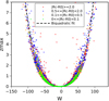 |
Fig. 1. Maximum height zmax (kpc) in terms of the vertical heliocentric velocity W (km s−1), with the biquadratic fit of Paper I (discontinuous line). The distance to the local radius is indicated in the colours. |
Similarly, in Fig. 2, the left panel shows two main features: the first, close to the origin, indicates that the relationship is nearly linear, but this trend is progressively lost. The other is that this loss is accompanied with an increasing dispersion of dots, which is greater for the stars that are more distant to the solar position. The latter feature is much more noticeable if the vertical eccentricity is used instead of the maximum height, as displayed in the right panel of Fig. 2 (the vertical eccentricity has been multiplied by r0 in order to compare with the graph plotted in terms of zmax).
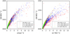 |
Fig. 2. Squared vertical peculiar velocity (W − W0)2 (km2 s−2) at the GP in terms of (left) the squared maximum height, |

We must recall that zmax is not an observable, while the vertical velocity is indeed such, with a relatively small error. The values to compute the orbital eccentricities, namely, ra, rp (maximum and minimum orbital distances to the centre, i.e., the apo- and pericentric distances), and zmax resulted from the numerical integration of each star orbit. In Paper I, we used the model of the Milky Way proposed by Ninković (1992) and assuming three contributors to the potential of the Milky Way: the bulge, the disc, and the corona. The contributions to the Galactic potential of the former two were described by the same formula as that of Miyamoto & Nagai (1975), with the only difference related to the values of the parameters. The parameters from Gaia DR2 (five-parameter astrometry solution and radial velocity) were used as inputs for the model and the integration of the Galactocentric orbits for each star was done for 10 Gyr by using a fourth-order Runge–Kuta method.
Depending on the approximated model, in the integration process, the stars whose values for ra or rp are more distant to the solar radius, r0 may accumulate a larger error. On average, it generally occurs that the greater the distance between the mean radius  of the orbit and r0, the greater the error.
By assuming the model is enough accurate, if the vertical velocity of a star is actually measured at the GP, we may determine the maximum height with a relatively small error3. However, if a star is not exactly at the GP, the vertical speed will be slightly lower and the maximum height is underestimated. For this reason, to determine the MVC, we should approximate the upper envelope of the set of dots in Fig. 2.
On the other hand, by using the vertical eccentricities instead of maximum height, we even get a better fit for the stars whose mean orbital radius, rm, is closer to (or larger than) the solar position, r0. However, for stars with rm < r0, the dispersion is much larger.
Let us remember that under the epicycle approximation, the orbit of a neighbouring star oscillates around the local circular velocity point, 𝒞 with radius rc ≈ r0. The following ratios:
define the planar and vertical orbital eccentricities of the star, respectively, which, in Paper I were used to associate the star with one of the local kinematical stellar populations. Under this approach, the value rc matches the value rm. Most stars of our working sample satisfy rm ≈ r0, which is consistent with the epicycle approximation. In such a case, the orbital eccentricities provide a homogeneous measure of the planar and vertical orbital amplitudes, allowing us to determine the planar and vertical epicycle frequencies. However, there are anomalous stars in the sample whose orbits oscillate around a value of rm that is significantly different from r0. For these stars, the local epicycle approximation is not appropriate. Obviously, the deviation from the epicycle model increases depending on whether the stars belong to the thin disc, the canonical thick disc, the metal-weak thick disc, the metal-rich thick-disc stars, or the halo.
We discuss (at the end of Sect. 3.3) why in the planar directions this fact is avoidable and why, in the vertical direction, it becomes necessary to distinguish between the actual vertical eccentricity  of such an anomalous star, which is referred to a circular velocity point different from the local one and the ratio
  this star provides. Therefore, the stars with rm < r0 have larger vertical eccentricities than the stars with the same zmax and a guiding circular orbit near r0. In other words, the former stars have an overestimated vertical eccentricity compared to the latter ones. On the contrary, the stars with rm > r0 have underestimated vertical eccentricities, but these lower values correspond to the domain closer to the origin, where the MVC is nearly linear and the dispersion of dots is not noticeable. Therefore, when working from vertical eccentricities, we should also fit the upper-left envelope of the set of dots in Fig. 2.
3.1. Interpretation of the maximum velocity curve
In order to be able to qualitatively interpret the MVC, we compare the potential of the harmonic oscillator with that of the Duffing oscillator (McLachlan 1950, p.24),  ; A > 0, B ≠ 0. This simple model is an example of a non-linear restoring force,
  ,
,  , such as a (unit) mass-spring system without damping, where the characteristic of the spring is f(z) = Az + Bz3. Another case of a similar non-linear restoring force is that of a mass at the centre of a taut, uniform vertical wire.
If B > 0, we get a slight modification of the harmonic oscillator, where the effective length of the spring decreases with increase in the amplitude of vibration. The stiffness is defined to be the derivative of the restoring force, i.e.,  . Thus, the stiffness indicates whether the potential function ϕ(z) is a convex or concave curve, so that the stiffness increases (convex) or decreases (concave) with increase in the displacement. In the current example, according as B > 0 or B < 0. For B > 0 all solutions are periodic around a single equilibrium point, but for B < 0 there exist periodic solutions around one equilibrium point only for
  . The other two fixed points are unstable.
For the Duffing oscillator, Eq. (3) becomes  . Figure 3 (right) shows such a curve for values B > 0 (red) and B < 0 (blue) (within the range of the periodic solutions), associated with the shape of the corresponding potential (left).
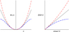 |
Fig. 3. Duffing potentials (left) with B > 0 (red) and B < 0 (blue) compared to the harmonic potential (grey). Maximum velocity curves (right) associated with these potentials. |
Since (according to Eq. (1)) the curvature of Z(0)2 is similar to that of 𝒰(zmax), from Fig. 2 (left panel) we can interpret the local neighbourhood by considering whether the stiffness decreases with increase in the maximum height. In other words, a potential provides decreasing stiffness if, for the same velocity Z(0), it is possible to reach higher values of zmax than for the harmonic potential.
Let us evaluate the potential function that is consistent with the local MVC.
3.2. Local constants
In order to determine a potential that allows us to fit the actual velocity curve, we study a family of potentials related to Eq. (2), which is more general than the cases previously analysed, where F is a rational function consisting of the ratio of two homogeneous polynomials of degree 2,
While the case (a) in Sect. 2 corresponds to a constant F, the cases (b) and (c) are particular cases4 related to Eq. (7). There are nine possible meaningful cases of Eq. (7), depending on whether in the numerator and in the denominator only one or none of the parameters are null. Indeed, there are not four free parameters in Eq. (7), since at least one parameter in the numerator and one in the denominator are not null, so that the ratio may be simplified. Hence, there are at most three free parameters that remain, which can be represented by the values F(0), F′(0), and F″(0).
The three local Galactic constants at the circular velocity point r = rc, z = 0, are related to the values  ,
,  , and
, and  , which, in turn, depend on M, F(0) and F′(0). To adjust the shape of the MVC, say its concavity, we also need to control the parameter F″(0).
We study the general case of Eq. (7), where a1, a2, a3, a4 are non-null. To this purpose, we write Eq. (7) in a more simple form, as follows:
so that

In Appendix A, we can see how the constant M in Eq. (2) is related to the planar epicycle frequency κ and the constant A in Eq. (8) is related to the angular velocity Ωc through the ratio

and both are involved in the planar motion of the stars. On the other hand, in Appendix B we see how the constant B is related to the vertical epicycle frequency ν, which is involved in the vertical motion of the stars.
3.3. Planar motion
Under the epicycle approximation, a star orbit can be referred to the circular motion point 𝒞 as

where a is the amplitude and p the phase. As a first approximation, we assume that Uc = U0 and Vc = V0, i.e., the circular motion point coincides with the local centroid. For disc stellar samples, this assumption is generally satisfied in the radial and vertical directions. For the rotation component, a priori, it is satisfied for low eccentricity stars, that is, for thin disc stars; otherwise, the asymmetric drift Δ = Vc − V0 should be considered in order to get a more accurate model. Therefore, under the first-order epicycle approach, the following should be satisfied:

Clearly, since a = rc e, this equation can be expressed in terms of the planar eccentricity, as in Paper I (Eq. (14)). There, it was fitted for several subsamples drawn from the current Gaia sample. We obtained stable estimates by basically removing the counter-orbiting stars of the halo. The average values for our working sample are  , κ ≈ 37 km s−1 kpc−1, Uc = U0 ≈ −10 km s−1, and Vc = V0 ≈ −20 km s−1, all of them consistent with the values that are usually assumed.
It is worth noticing that the planar fitting did not need the correction for the asymmetric drift. The reason is as follows: The above ellipses describe the motion of the stars referred to their circular velocity point, which, as commented at the beginning of Sect. 3, not always match the local one, rc. Nevertheless, the local constants γc and κ should not differ very much from point to point. The former depends on Ωc, which, while it is not constant, its variation is relatively small around the Sun, since it satisfies  . The latter does not depend on rc. Therefore, the respective data, even for different circular velocity points, could be gathered as a single fitting.
3.4. Vertical motion
By taking Eq. (B.4)into account, the MVC given by Eq. (3) can be written, for r = rc, as

We note the local linear behaviour in the squared variables that satisfies
Therefore, we want to determine the above function w2(zmax, rc) at the local position rc = r0. Since the remaining values Wc ≈ −6 km s−1 and ν ≈ 63 km s−1 kpc−1 of Paper I for the current sample are still valid, it is sufficient to estimate the constant C.
Nevertheless, we must remark that a part of the stars in the sample (ca. 25%) have a value for rm that is more than 1 kpc away from the local radius r0 – we assume that this value matches the average radius of the sample, r0 ≈ 8.3 kpc, which is similar to that of Reid et al. (2014). Thus, their orbit cannot be strictly referred to the local circular velocity point. As already explained, Eq. (13) should be adjusted only for the stars with rm close to r0, namely, the green and orange dots in Fig. 1, but in order to use all the available data, we fit the upper envelope of the whole set of dots.
Instead of making an adhoc geometrical approximation, in Appendix C we propose a more rigorous fitting method. As a result, we get the (dimensionless) value C = 21 ± 1. We discuss some of the consequences this value has on the potential in Appendix D.
4. Results
4.1. Eccentricity diagram
In the solar neighbourhood, according to Eq. (13) and by taking rc = r0 and ν ≡ ν(r0), the vertical peculiar velocity of a star depends on its vertical eccentricity as

By inverting the above equation, we may estimate the vertical eccentricity of a disc star that has a vertical peculiar velocity w at the GP, obtaining the following positive solution,
Hence, the least squares fitting of Eq. (5) must be replaced by the estimation provided by Eq. (15), while including the fitting of the upper envelope.
In Paper I, we found four regions of the eccentricity diagram, e′2 vs. e2, corresponding to subsequent nested populations contained in the working sample. These populations were obtained from stellar subsamples selected from specific sampling parameters, as indicated in Table 1. In particular, the thin disc was associated with region R2 (selected from |v|≤230 km s−1) and the whole disc with R4 (selected from |W|≤130 km s−1, although the subsample with |W|≤170 km s−1 provided a slightly lower χ2 error). By using the current approach, the estimations for the limiting eccentricities of the nearly triangular regions R1 to R4 can now be determined with greater accuracy, in particular for the stars with velocity satisfying |v|> 50 km s−1.
Parameters delimiting the triangular regions Ri according to the stars’ orbital parameters.
We reevaluate these regions. Thus, Eq. (21) in Paper I should be replaced by the following one5, in terms of Eq. (14),
The above equation determines an area similar to a quarter ellipse as in Paper I (Eq. (23)), which can be approximated by the following one,

where B2 replaces the value B1 of Paper I. The constant B2 is evaluated as follows. In Eq. (17), for e = 0, the maximum vertical eccentricity ζ satisfies g(ζ2) = NB0. Then, B2 = ζ2. Thus, by writing it explicitly, according to Eqs. (15) and (16),
Therefore, the limiting (squared) vertical eccentricity B2 is determined from the velocity dispersions of every two adjacent populations, together with the constants K, N and C, where the latter adjusts the curvature of the MVC estimated from the envelope of the vertical speeds in crossing the GP.
Table 1 shows the values A0, B1 and B2. For the planar motion, the estimations A0 are the same as in Paper I. For the vertical motion, the estimations B1 are those of Paper I and B2 are the new ones, obtained from the potential model.
According to the above equations, Fig. 4 compares the new (blue) regions R2 and R4, corresponding to the borders of the thin and thick discs, with the ones obtained in Paper I (green). The continuous curves represent the corresponding model (either the biquadratic fit of Paper I or the model from the local potential), while the doted curves are the respective approximations from quarter ellipses. The small red doted curves feature the first-order epicycle approach. The set of curves closer to the centre determine the region R2, while the farthest determine the region R4.
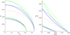 |
Fig. 4. Quarter ellipses (left) defining the regions R2 (closer to the origin) and R4 (farther from the origin), according to the biquadratic fit (continuous green curves), potential model (continuous blue curves), and epicycle approach (dotted red curves). The dotted green and blue curves are the respective approximations from quarter ellipses. The same regions in terms of the squared eccentricities are displayed on the right. |
The resulting eccentricity diagram for the current stellar sample is shown in Fig. 5 for the triangular regions of Eq. (18).
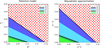 |
Fig. 5. Triangular regions according to Table 1, for the current potential model (left) and for the biquadratic approximation (right). The complementary area is the halo (red). |
When the stars are labelled according to the region their eccentricities belong to, we obtain the diagram of Fig. 7 (left). If the number of stars in a region Ri that do not belong to the regions Rj, for j < i, is denoted as Ni, and the corresponding population component as Pi, we get, for the current potential model6,

We note that these fractions do not denote areas but number of stars in the sample that fall in the corresponding region.
Populations P1 (light green area) and P2 (dark green) are associated with the thin disc, although the second subcomponent is mixed with some thick disc stars. The thick disc is composed of the canonical subcomponent P3 (light blue) and the metal-weak thick disc P4 (dark blue). The kinematical halo stars present in the sample, P5, probably are a mixture of metal-rich thick-disc stars and chemical halo stars (Di Matteo et al. 2019).
By comparing the actual stellar classification to that of Paper I, we find that the thin disc has now 1.5% less stars (mainly due to the major subpopulation P1), while the thick disc has increased 10% relative to the same population in Paper I. This is due to the smaller maximum height now associated with these populations (Table 1), which is more noticeable in the larger population. Thus, the current approach provides a 10–15% thinner disc.
The respective population mean velocities and velocity moments are listed in Table 2. The resulting velocity moments for the thin disc are similar to those Paper I, with velocity dispersions (σ1, σ2, σ3) = (30.4, 19.7, 13.8) km s−1, while those of the thick disk, (59, 35.7, 35.3) km s−1, are slightly lower than those in Paper I, (60.9, 36.3, 36.6) km s−1, since stars previously assigned to the thin disc are now labelled as thick disc.
Mean velocities, central moments, and population fractions (relative to the whole sample) from the eccentricity diagram.
4.2. Asymmetric drift
As an application of the eccentricity diagram, here we analyse deeper samples of the thin disc by selecting stars within concentric ellipses, closer to the origin, corresponding to the thin disc, namely, region R1. We test the disc components with regard to the asymmetric drift. Let σ2 be the trace of the velocity dispersion tensor, namely,  . Strömberg’s asymmetric drift equation (e.g., Binney & Tremaine 2008) predicts that the larger a stellar population’s velocity dispersion, the more slowly it rotates about the GC. There is a linear relation between the peculiar rotation velocity, V0, of a stellar population and the total velocity dispersion given by σ2 and, in particular, by μ200, except for very early-type stars (Dehnen & Binney 1998). However, we find that the trend for the thin disc is different than from the thick disc. To prove it, we take advantage of the eccentricity diagram and form several nested subsamples within the thin disc, according to the stars’ eccentricities. We limit the maximum planar and vertical eccentricities following Eq. (18), by taking as reference values those limiting the region R1 of Table 1. Hence, we consider the subsamples that satisfy:
The value i = 0 corresponds to region R1, while higher values of i correspond to smaller ellipses within R1. We also consider the remaining disc samples of regions from R2 to R4. We find that the samples for i = 0, 1, 2, 3, corresponding to limiting eccentricities  , (0.23, 0.065), (0.19, 0.053), (0.15, 0.043) provide stable velocity moments; whereas for i = 4, 5, 6, corresponding to limiting eccentricities
  , (0.10, 0.029), (0.08, 0.024) do not yield stable estimates. Hence, the subsamples of the lowest eccentricities reflect the kinematics of the local moving groups and star streams, as explained in Cubarsi (2010), rather than being statistically representative of the thin disc population. Therefore, we use the disc subsamples listed in Table 3.
Figure 6 (top-left panel) shows such a trend for the thin disc subsamples (black dots), as well as for the segregated populations P1 and P2 (green dots). The dots without colour, for the samples containing thick disc stars, deviate from the regression line. In terms of the heliocentric rotation velocity V0, the total dispersion σ2 (with slope −4105 ± 75 km s−1) and the moment μ200 (with slope −2621 ± 83 km s−1) allow us to estimate the heliocentric velocity of the circular rotation point as Vc = −12.81 ± 0.06 km s−1 and −12.99 ± 0.09 km s−1, respectively. For these subsamples, the following is approximately satisfied: σ2/μ200 = 1.58 ± 0.02.
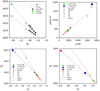 |
Fig. 6. Strömberg’s law and asymmetric drift equation adjusted for several subsamples. Top: Strömberg’s law for thin disc subsamples (black dots) accounting for the total velocity dispersion σ2 (km2 s−2) and the velocity moment μ200 (km2 s−2) in terms of their heliocentric rotation velocity V0 (km s−1). Fitting of Eq. (21) (right panel) for thin disc subsamples (red dots) using the optimal value of γc. Bottom: (left panel) Strömberg’s law for the total thin disc (t, red line) and the thick disc (T, black line) subsamples; and (right panel) for thin disc, thick disc, and halo (H) components. |
The value for Vc is totally consistent with that obtained from the chemodynamical model by Schönrich et al. (2010) and differs from the one given by Golubov et al. (2013), derived from subsamples obtained from the RAVE survey (Siebert et al. 2011; Zwitter et al. 2008; Steinmetz et al. 2006). We note that our subsamples are representative of the thin disc kinematics, having values for μ200 as low as 420 km2 s−2, while the sample values of Golubov et al. (2013) for this moment vary approximately from 700 to 1500 km2 s−2. This fact is indicative that such samples also contain either thick disc stars, metal-weak thick disc, or metal-rich thick-disc stars.
When these stars are included in our fitting, the trend of Strömberg’s law is slightly modified, as shown in Fig. 6 (left lower panel, black line for the thick disc and red line for the thin disc). By using σ2, the line that fits the thick disc population (T = P3 + P4), the regions R3 and R4 (which contain thick disc stars), and the whole thin disc (t = P1 + P2) intersects the horizontal axis at −10.5 ± 0.1 km s−1. This value is maintained (−10.4 ± 0.1) if the halo population is included in the fitting (right lower panel, black line).
By assuming an average value Vc ≈ −12.9 km s−1 we may evaluate the drift Δ2 = Vc − V0 for each thin disc subsample. Under the first-order epicycle approximation, for low eccentricities, the asymmetric drift is neglected and it is approximately satisfied  . Under a more general model that does not neglect the asymmetric drift, the following is fulfilled (Cubarsi et al. 2017, Eq. (70)):
where the difference Δ1 = Uc − U0 can be considered null for the thin disc subsamples, since the radial mean velocity is nearly constant. Therefore, we may estimate the local value  providing the best approximation of Eq. (21). The value that fits the local thin disc subsamples is
  . The plot in the top-right panel of Fig. 6 displays such a fit. This value is slightly higher than the one derived in Paper I for all the working sample (
 ), obtained by limiting the vertical velocity of the stars as |W|≤170 km s−1, although it is similar to that of the thin disc sample, whose stars satisfied |W|≤35 km s−1 (
 ). Therefore, we get an approximate estimation of the asymmetric drift for thin disc stars from the equation
so that, if Δ2 → 0 then σ1/σ2 → γc ≈ 1.48 (although, for samples containing thick disc stars, this ratio is closer to 1.4).
The absolute rotation velocity of the circular orbit can be estimated from Eq. (10) as  km s−1, which provides a rotation component of the Galactocentric velocity of the Sun Θ⊙ = Θc − Vc ≈ 240 km s−1.
5. Discussion
In the left panel of Fig. 7, we show the eccentricity diagram for the triangular regions obtained from the approximation given by Eq. (18). We compare it to the right panel, where the eccentricity diagram is depicted exactly, as obtained7 from Eq. (17). The approximation from triangular regions is very exact for the thin disc, which represents the great majority of the stars in the sample. In all the disc populations, the variation is of less than 0.5%. Therefore, approximating by triangular regions is fully justified.
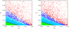 |
Fig. 7. Triangular regions R1 to R4 for the actual eccentricities (as depicted in Fig. 5) obtained from Eq. (18) (left), and exact regions (right) obtained from Eq. (17). |
In order to check whether the current approach provides a reliable method to isolate populations, we infer the planar and vertical eccentricities of the stars in the sample from the stars’ velocities, according to Eqs. (12) and (15). That is, we do not use the actual eccentricities obtained by integration of the orbits, but the ones estimated from our approach. In order to see how they are reorganised, Fig. 8 depicts the eccentricity diagram for the same stellar populations as the left panel of Fig. 7, but while including the modified eccentricities. For the highest eccentricities, the plot describes the small curvature predicted in Fig. 4, which is similar to that of the right panel of Fig. 7. The diagram shows that most of the populations are generally well isolated, that is, without significant overlapping areas. However, there is a small mixing at the borders between the regions, which corresponds to the tails of the respective velocity distributions, as discussed in Paper I.
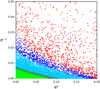 |
Fig. 8. Regions R1 to R4 according to the eccentricities obtained from Eqs. (12) and (15), in terms of the star’s velocities. |
Once the stars in the sample have been assigned to one of the populations components, we check which stars are better described by the MVC. Figure 9 displays the vertical peculiar velocity in terms of the maximum height and of the vertical eccentricity. In both cases, the curve, which is the upper envelope of the dots, fits the stars of populations P1 and P2 of the thin disc well, and also provides an acceptable fit for the old thick disc stars of population P3. For population P4, as the eccentricity increases, the dots become more dispersed. Clearly, the model is not valid for the halo stars. There are several reasons for this. One is that for the halo, the epicycle approach is not valid. Another reason is that, by comparing Figs. 2 and 9, most of the halo stars have the mean orbital radius farthest from the local one, so that the eccentricities are not referred to the local circular velocity point. Also, according to Paper I, in the halo there is a fraction of counter-rotating stars for which the planar fitting was not valid. There is also a possible dispersion that can be attributed to uncertainties in the computation of the orbital parameters, along with other uncertainties and errors discussed in Paper I. All these reasons do not invalidate the local approximation we make for the MVC, since the vertical velocity at the GP should determine univocally the maximum height of the star orbit. With the exception of the halo stars, the fit is more precise in the plot in terms of the eccentricity (right panel) than in terms of the maximum height (left panel).
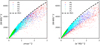 |
Fig. 9. Squared vertical peculiar velocity (W − W0)2 (km2 s−2) at the GP in terms of (left) the squared maximum height |

The curvature of the MVC is regulated by the vertical epicycle frequency at the origin, and by the constant C far from the origin. The latter constant adjusts the stiffness in the vertical direction of the oscillator associated with the potential. The shape of the MVC is similar to that of Fig. 3 with B < 0, associated with a decreasing stiffness.
Let us recall that the constants involved in the potential function, combined with the velocity dispersions of every two adjacent populations, determine the border between these populations in the eccentricity diagram. In particular, in the following subsections we analyse how, in the vertical direction, the maximum height and the maximum speed of disc stars depend on the constant C. The approximation of the MVC based on the potential allows us to interpret qualitatively several aspects, such as what behaviour of the MVC can be attributed to the disc or the halo. A similar effect is observed with regard to the stellar density. On the contrary, the approach in Paper I, associated with an arbitrary biquadratic function, was not liable to such speculation.
5.1. Disc and halo contributions
On the one hand, the constants M and A are linked to properties of the planar motion, i.e., the planar epicycle frequency κ and the local angular velocity Ωc. On the other hand, the constants B and C are related to properties the vertical motion, i.e., the vertical epicycle frequency ν determining the tangent at the origin, and the curvature of the MVC. We now write Eq. (13) as:
By defining
the preceding equation becomes

Here, the factor within the parenthesis can be interpreted as a weighted mean of the following limiting cases:
-
(1)
Stars with low values of e′ (say disc stars). In particular, if e′ → 0, then g1(e′2)→1 and g2(e′2)→0. Hence, the dominant term in Eq. (24) is (blue-dashed line in Fig. 10) is
-
(2)
There is a harmonic term of the potential, which, according to Eq. (A.2), is related to κ. It corresponds to an ellipsoid of constant density. The corresponding term in Eq. (24) is relevant for stars with higher values of e′ (say halo stars). If e′ → ∞, then g1(e′2)→0 and g2(e′2)→1. In this case, the dominant term is (red-dashed line in Fig. 10)
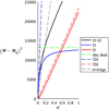 |
Fig. 10. Contribution of the disc and halo components to the maximum velocity curve, i.e., local vertical peculiar velocity w = W − W0 (squared, km2 s−2) at the GP in terms of vertical eccentricity e′ (squared, dimensionless). The continuous lines correspond to the whole curve (black), the disc term (blue), and the halo term (red). The dashed blue and red lines are the respective tangent (TD) and asymptote (TH), the dashed grey line is their geometric mean, and the dashed green line marks the bound for the vertical speed (squared) of disc stars. |
The total trend of Eqs. (23) and (24) is shown in Fig. 10 by the continuous black line, while the disc (first term of Eq. (23)) is represented by the continuous blue line, and the halo (second term of Eq. (23)) by the continuous red line. The curve is modulated by e′2 between both straight lines, one is the tangent for e′ → 0, with slope  (dashed blue line), and the other is the asymptote for e′ → ∞ (actually, it is sufficient for e′ → 1), with slope
  (dashed red line).
The term g1, associated with the disc, governs the curve for  , namely, for z < z0 with

For the actual values, this means z0 ≈ 1.8 kpc. We should expect that the maximum heights zmax of the disc subpopulations satisfy zmax < z0. Otherwise, for z > z0, the dominant term is g2, associated with the halo.
If  , bearing in mind Eq. (13) and according to the assumptions presented in Sect. 3.1, the stiffness decreases with increase in the maximum height and vertical eccentricity. This is the actual case. Otherwise, the stiffness would increase with increase in the maximum height and vertical eccentricity. Since a straight line means constant stiffness, the progressively decreasing stiffness only takes place in the range of low eccentricities, namely, for the disc stars. Afterwards, as the vertical eccentricity increases, the curve takes the asymptotic behaviour, where the stiffness remains constant. This happens as the term
  gets closer to its saturation value (it suffices for e′ → 1),

which is indicated by the dashed green line in Fig. 10, while the term associated with the halo continues to rise. Therefore, such a value can be interpreted as the upper limit for the maximum vertical velocity of the disc stars. In Appendix E, we describe some properties of the slope of the curve in more detail.
According to our estimates, this provides a maximum vertical peculiar velocity W − W0 = w0 ≈ 115 km s−1, which is consistent with the value of the sampling parameter |W| = 130 km s−1 (vertical heliocentric velocity) with which (in Paper I) it was possible to establish the segregation between the disc (as population 1) and the halo (as population 2). In such a case, for greater values of the sampling parameter, the velocity moments of the disc remained approximately constant (Paper I, Fig. 2).
In Fig. 11, the discontinuous grey line represents the term corresponding to g1 in Eq. (24), which provides the saturation value, the continuous black line represents the relationship between the maximum height provided by the potential model, and the discontinuous red line corresponds to the biquadratic fit of Paper I, given by Eq. (5).
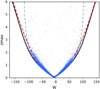 |
Fig. 11. Maximum height zmax (kpc) in terms of the vertical heliocentric velocity W (km s−1) according to different approaches: continuous black line for the model provided by the local potential, discontinuous red line for the biquadratic fit of Paper I, and discontinuous grey line for the disc component alone. |
The condition  is satisfied for
  (
( ). This corresponds to a maximum height zmax ≈ 1.5 kpc of the region of decreasing stiffness. From this value onward, the curve becomes nearly a straight line. The value z0 is approximately the maximum height for the whole disc R4.
Therefore, the disc stars have a bound for their maximum vertical speed w0 at the GP. For a given speed, they are able to reach certain maximum height z0, which would not exist for a potential harmonic in the variable z (i.e., C = 0). Nevertheless, the progressive weakening of the stiffness within the disc is compensated by the halo, which produces a total curve also with decreasing stiffness, but which is not as intense. Therefore, the halo contributes to stabilise the stellar orbits. We consider how the maximum height of the disc depends on C in more detail in the following subsection.
5.2. Stellar density
We analyse how the constant C is related to the stellar density. Poisson’s equation, Δ𝒰(r, z) = 4πGρ(r, z), relates the potential and the density at a point. The density for r = r0 in terms of z is obtained in Appendix F, by substitution of the potential of Eq. (2) in Poisson’s equation. According to this simplified model, the shape of ρ0(z) ≡ ρ(r0, z) is displayed, for positive values of z, in Fig. 12 (blue line). It is also compared to other values for C, to show how the local minimum depends on this parameter. The local minimum with vanishing density determines the maximum height z0 of the disc.
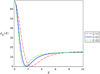 |
Fig. 12. Density ρ(r0, z) = ρ0(z) (×106 M⊙ kpc−3) in terms of z (kpc) for C = 21 (blue), compared to other values of C. |
In Appendix F, the value of z0 is given by Eq. (F.3), together with two approximations. One of them, Eq. (F.4), matches that of Eq. (25), derived from the analysis of the MVC.
Figure 13 displays (left panel) the value z0 in terms of C (blue curve), as well as both approximations (dotted red and green curves). Both approximations are valid within a wide interval about the estimated value for C. Figure 13 also displays (right panel) the maximum velocity w0 of disc stars provided by Eq. (26). The grey dashed lines mark the values for C = 21, namely, z0 = 1.8 kpc and w0 = 115 km s−1.
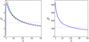 |
Fig. 13. Maximum height (left) z0 (kpc) in terms of C (blue curve) from Eq. (F.3), compared to the approximations from Eq. (F.4) (green, similar to Eq. (25)) and Eq. (F.5) (red). Maximum vertical peculiar velocity (right) of disc stars w0 (km s−1) from Eq. (26). The dashed grey lines mark the estimated values, z0 = 1.8 kpc and w0 = 115 km s−1, for C = 21. |
Therefore, the constant C, which regulates how the stiffness decreases with increase in the maximum height, also determines the limiting disc values for z0 and w0. The greater the value of C, the greater the descent of the stiffness and the lower the values of z0 and w0.
With regard to the stellar density, Fig. 14 displays several properties. We consider the number of disc stars within a column or cylinder perpendicular to the GP, of unit area, for r = r0 and z ∈ [ − z0, z0], namely:
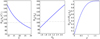 |
Fig. 14. Function D0(z0) (×106 M⊙ kpc−2) plotted in terms of C and z0 (left and central panels). The dashed grey lines mark the estimated values for C = 21 and z0 = 1.8 kpc. Fraction of stars with |z|≤z0 relative to the number of stars with |z|=z0 is given in the right panel. |
The left and central panels of Fig. 14 depict the above density in terms of C and z0. For the maximum height z0, within the range of values 1.5 < z0 < 2.8 (corresponding to the interval 9 < C < 30) this variation is nearly linear.
The right panel depicts the fraction of stars within the interval [ − z, z] ⊂ [−z0, z0], relative to the number of stars in the interval [ − z0, z0], that is, the ratio D0(z)/D0(z0). By comparing the value D0 for zmax = 1.5 kpc (which was the maximum height estimated for the disc from the velocity analysis of our working sample) with the value D0 for z0 = 1.8 kpc, we get a ratio 99.5%. Therefore, both estimations of the maximum height of the disc provide a similar number of stars in the local cylinder. Indeed, according to this model, for C = 21, a fraction of 95% of the disc stars are in the range of |z|≤1.1, and 66% of the disc stars are in the range of |z|≤0.55, which is consistent with the current sample. The ratio D0(z)/D0(z0) is nearly linear for |z|< 0.6 kpc.
We may also compare the above estimations to those obtained for a value C = 15, which would produce a lower decrease of the stiffness. Then, the maximum height would be z0 = 2.1 kpc and the limiting velocity w0 = 135 km s−1, while the local density of the disc cylinder increases in about 15%. In such a case, 95% of the disc stars satisfy |z|≤1.3, and 66% have |z|≤0.65. Thus, as shown in to Fig. 15, a decrease of about 15% in the limiting velocity w0 (similar for the value z0), would produce a quite similar decrease, of about 14%, in the density D0 of the local cylinder. Then, the approximate local behaviour in the disc can be described so that a greater decrease of the stiffness in a certain ratio is associated with a decrease in the limiting velocity that produces a thinner disc and a loss of stars of the local cylinder, which become unbound in a similar proportion. This loss is distributed among all values of z, as Fig. 12 suggest. Therefore, the loss of stiffness within the disc can be interpreted as whether there is not enough mass in the disc to keep the stars bounded, although this effect is afterwards mitigated by the halo.
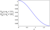 |
Fig. 15. Relative decrease of density in the local cylinder in the range [ − z, z] (kpc), when comparing a disc model with velocity limit w0 = 115 km s−1 (z0 = 1.8 kpc) to another one with w0 = 135 km s−1 (z0 = 2.1 kpc). |
Let us point out that the requirements for our potential have been, on the one hand, to allow for a finite mixture of independent Schwarzschild velocity distributions and, on the other hand, to be consistent with the kinematic statistics estimated from our local sample. It is generally known that, according to an assumed potential, Poisson’s equation allows us to estimate the mass density generating such a potential. However, such a stellar density will not match the sum of the stellar densities of the n populations involved in the mixture model. If the ith population has a population fraction ni and a velocity distribution fi, its density is evaluated as Ni = ∫Vfi dV, so that the contribution of all the populations to the total density is ∑iniNi (each population has a stellar density according to Cubarsi (2014a, Eq. (40)). However, in addition to the stars in the sample, there is an unknown amount of stars and, in general, dark matter that has not been considered – even though all of these factors contribute to the potential.
6. Conclusions
In Paper I, we proposed an approach to classify the local stellar populations in terms of the stars’ planar and vertical orbital eccentricities. Such a classification was characterised by a geometrical interpretation associated with regions delimited approximately by a straight line in the eccentricity diagram, namely, the plot of the squared vertical eccentricity in terms of the squared planar eccentricity.
According to Paper I, in the GP the planar eccentricities described consistently the planar velocity distribution of the stars. However, upon moving away from the GP, the vertical epicycle approximation was no longer valid and required a better approximation model. In this work, we improve such an approximation by taking into account a plausible model for the local potential function, making it possible to elicit several properties, such as the maximum height of disc stars and their maximum speed in crossing the GP.
We consider a kinematical stellar population as a sufficiently large number of stars whose velocity distribution is trivariate Gaussian, and we take the potential to be consistent with an unconstrained mixture of populations (Cubarsi 2014a). Within this family, potentials with spherical symmetry or separable in cylindrical coordinates are unable to fit the model. Therefore, we consider a model that allows us to evaluate, in addition to other local Galactic constants, the curvature of the MVC, associated with a constant C, which determines the possible regions where the non-harmonic part of the potential generates an attractive or a repulsive force. Our fitting method yields the value C = 21 ± 1, always generating an attractive force.
In the vertical direction, we have taken the Duffing oscillator as a model of a non-linear restoring force. The shape of the MVC is similar to the model of Fig. 3 with B < 0, associated with a decreasing degree of stiffness. In the local neighbourhood, we can interpret it so that the stiffness decreases with increase in the maximum height. Hence, for the same vertical velocity, it is possible to reach a higher maximum height than for the harmonic potential.
In particular, the constant C determines the limiting maximum height, z0, and the maximum speed at the GP, w0, for the disc. The greater the value of C, the greater the descent of the stiffness, and the lower the values of z0 and w0. With regard to the local stellar density, this is expected to produce a thinner disc and a loss of disc stars of the local cylinder.
The improved model allows us to reevaluate the critical planar and vertical eccentricities in the eccentricity diagram in order to discriminate between the different kinematic populations contained in the current Gaia local sample. The thin disc is described by the quarter ellipse satisfying
that is, for 0 ≤ e ≤ 0.32, 0 ≤ e′ ≤ 0.09, with a maximum height zmax = 0.73 kpc. The whole disc is described by the region satisfying
that is, 0 ≤ e ≤ 0.44, 0 ≤ e′ ≤ 0.18, zmax = 1.50 kpc. We confirm that the approximation of the eccentricity diagram from triangular regions is very accurate and there is no need of using the exact representation from Eq. (17).
Therefore, the vertical values obtained for the biquadratic approximation of Paper I were slightly overestimated. By comparing the current stellar classification, we find that the thin disc (88%) of our local sample now has 1.5% fewer stars, while the thick disc (9%) has increased relatively in 10%. In total, a 3% of stars were misclassified by the previous approach among populations P1 to P5. However, such a variation has a low impact on the velocity moments, with velocity dispersions (σ1, σ2, σ3) ≈ (30, 20, 14) and (59, 36, 35) km s−1 for the thin and thick discs, respectively. Nevertheless, the current approach provides a 10−15% thinner disc.
As an application of the eccenticity diagram, we analysed several nested subsamples within the thin disc to estimate Strömberg’s asymmetric drift equation. The thin disc is well represented from samples with limiting eccentricities 0.15 ≤ emax ≤ 0.32,  in the eccentricity diagram. Lower-limiting eccentricities did not yield stable estimates, but rather reflect the kinematics of the local moving groups and star streams (Cubarsi 2010). The trend for the thin disc is different from that by including thick disc stars. Within the thin disc, we have estimated the heliocentric velocity of the circular rotation point as Vc = −12.81 ± 0.06 km s−1, a value consistent with that obtained by Schönrich et al. (2010). Consequently, the absolute rotation velocity of the circular orbit has been evaluated in Θc ≈ 227 km s−1, which provides a rotation component of the Galactocentric velocity of the Sun Θ⊙ ≈ 240 km s−1.
In addition, we have provided an approximated formula, Eq. (21), to estimate the asymmetric drift Δ2 within the thin disc from the velocity dispersions σ1 and σ2, according to the optimal value for the constant γc = 1.48 ± 0.01. This value is slightly higher than the one derived in Paper I for all the working sample (γc = 1.40), obtained by limiting the vertical heliocentric velocity of the stars as |W|≤170 km s−1, although it is similar to that of the thin disc sample, whose stars satisfied |W|≤35 km s−1 (γc = 1.49). Thus, for the thin disc, we have, if Δ2 → 0, then σ1/σ2 → γc ≈ 1.48.
The interpretation of the MVC leads to a maximum vertical peculiar velocity for disc stars w0 = 115 km s−1, which is consistent with the limiting sampling parameter |W| = 130 km s−1 (vertical heliocentric velocity) used in Paper I to select a disc subsample. On the other hand, the potential together with the Poisson equation provide an upper bound z0 = 1.8 kpc for the disc, which is consistent with the maximum height estimated for the disc subpopulations of the working sample. Indeed, the a fraction of 95% of disc stars should be in the range |z|≤1.1 kpc, and 66% in the range |z|≤0.55 kpc.
At the moment, we have fulfilled the first purpose established in Paper I, which was to justify and improve the approximation of the MVC. In addition to maintaining the other purposes, we think that it might be worth studying how the approach improves by using a second order epicycle approximation, such as the one proposed by Kalnajs (1979). Likewise, we propose to explore other models for the integration of the stellar orbits. Similarly, to compare the behaviour of the MVC associated with other potentials, such as those listed in the galpy python package8, and study their consequences, namely, the mutual dependence between the maximum height of the disc, the vertical velocity limit, and the local stellar density.
The velocities of the stellar sample are given in a heliocentric coordinate system, with the radial heliocentric velocity component U positive towards the GC, the heliocentric velocity component V positive in the direction of the Galactic rotation, and the velocity component W perpendicular to the GP and positive towards the NGP. The velocity of the local centroid, i.e., the mean motion of the local sample, is expressed as (U0, V0, W0).
The case (b) corresponds to a1 ≠ 0, a2 = 0, and a3 = a4 in Eq. (7), and the case (c) to a1 ≠ 0, a2 = 0, and a3 ≠ a4, which is qualitatively equivalent to the case a3 ≠ 0, a4 = 0, and a1 ≠ a2.


Acknowledgments
The work presented in this paper was supported by the Ministry of Education, Science and Technological Development of the Republic of Serbia, Grant number 451-03-9/2021-14/200002 of Astronomical Observatory.
References
- An, J., & Evans, N. W. 2016, ApJ, 816, 35 [NASA ADS] [CrossRef] [Google Scholar]
- Binney, J., & Tremaine, S. 2008, Galactic Dynamics, 2nd edn. (Princeton: Princeton University Press) [Google Scholar]
- Chandrasekhar, S. 1942, Principles of Stellar Dynamics (New York: Dover Publications) [Google Scholar]
- Cubarsi, R. 1990, AJ, 99, 1558 [NASA ADS] [CrossRef] [Google Scholar]
- Cubarsi, R. 2010, A&A, 510, A103 [NASA ADS] [CrossRef] [EDP Sciences] [Google Scholar]
- Cubarsi, R. 2014a, A&A, 561, A141 [NASA ADS] [CrossRef] [EDP Sciences] [Google Scholar]
- Cubarsi, R. 2014b, A&A, 567, A46 [NASA ADS] [CrossRef] [EDP Sciences] [Google Scholar]
- Cubarsi, R., Stojanović, M., & Ninković, S. 2017, Serb. Astron. J., 194, 33 [NASA ADS] [CrossRef] [Google Scholar]
- Cubarsi, R., Stojanović, M., & Ninković, S. 2021, A&A, 649, A48 [CrossRef] [EDP Sciences] [Google Scholar]
- Dehnen, W., & Binney, J. J. 1998, MNRAS, 298, 387 [NASA ADS] [CrossRef] [Google Scholar]
- Di Matteo, P., Haywood, M., Lehnert, M. D., et al. 2019, A&A, 632, A4 [NASA ADS] [CrossRef] [EDP Sciences] [Google Scholar]
- Eddington, A. S. 1915, MNRAS, 76, 37 [NASA ADS] [CrossRef] [Google Scholar]
- Evans, N. W., Sanders, J. L., Williams, A. A., et al. 2016, MNRAS, 456, 4506 [NASA ADS] [CrossRef] [Google Scholar]
- Gaia Collaboration (Brown, A. G. A., et al.) 2016, A&A, 595, A2 [NASA ADS] [CrossRef] [EDP Sciences] [Google Scholar]
- Gaia Collaboration (Brown, A. G. A., et al.) 2018, A&A, 616, A1 [NASA ADS] [CrossRef] [EDP Sciences] [Google Scholar]
- Gaia Collaboration (Brown, A. G. A., et al.) 2021a, A&A, 649, A1 [NASA ADS] [CrossRef] [EDP Sciences] [Google Scholar]
- Gaia Collaboration (Smart, R. L., et al.) 2021b, A&A, 649, A6 [EDP Sciences] [Google Scholar]
- Gilmore, G., King, I. R., & van der Kruit, P. C. 1990, The Milky Way as a Galaxy, Advanced course of the Swiss Society of Astronomy and Astrophysics (University Science Books) [Google Scholar]
- Girard, T. M., Korchagin, V. I., Casetti-Dinescu, D. I., et al. 2006, AJ, 132, 1768 [NASA ADS] [CrossRef] [Google Scholar]
- Goldstein, H. 1980, Classical Mechanics, Addison-Wesley Series in Physics (Boston: Addison-Wesley Publishing Company) [Google Scholar]
- Golubov, O., Just, A., Bienaymé, O., et al. 2013, A&A, 557, A92 [NASA ADS] [CrossRef] [EDP Sciences] [Google Scholar]
- Kalnajs, A. J. 1979, AJ, 84, 1697 [CrossRef] [Google Scholar]
- Lynden-Bell, D. 1967, MNRAS, 136, 101 [NASA ADS] [CrossRef] [Google Scholar]
- Makarov, A. A., Smorodinsky, J. A., Valiev, K., & Winternitz, P. 1967, Nuovo Cimento A Serie, 52, 1061 [CrossRef] [Google Scholar]
- McLachlan, N. 1950, Ordinary Non-linear Differential Equations in Engineering and Physical Sciences (Oxford: Clarendon Press) [Google Scholar]
- Miyamoto, M., & Nagai, R. 1975, PASJ, 27, 533 [NASA ADS] [Google Scholar]
- Ninković, S. 1992, Ap&SS, 187, 159 [Google Scholar]
- Ogorodnikov, K. F. 1965, Dynamics of Stellar Systems (Oxford, UK: Pergamon Press) [Google Scholar]
- Oort, J. H. 1928, Bull. Astron. Inst. Neth., 4, 269 [Google Scholar]
- Pars, L. 1965, A Treatise on Analytical Dynamics (Hoboken: Wiley) [Google Scholar]
- Reid, M. J., Menten, K. M., Brunthaler, A., et al. 2014, ApJ, 783, 130 [Google Scholar]
- Sala, F. 1990, A&A, 235, 85 [NASA ADS] [Google Scholar]
- Schönrich, R., Binney, J., & Dehnen, W. 2010, MNRAS, 403, 1829 [NASA ADS] [CrossRef] [Google Scholar]
- Siebert, A., Williams, M. E. K., Siviero, A., et al. 2011, AJ, 141, 187 [NASA ADS] [CrossRef] [Google Scholar]
- Smith, M. C., Evans, N. W., Belokurov, V., et al. 2009, MNRAS, 399, 1223 [NASA ADS] [CrossRef] [Google Scholar]
- Steinmetz, M., Zwitter, T., Siebert, A., et al. 2006, AJ, 132, 1645 [Google Scholar]
- Zwitter, T., Siebert, A., Munari, U., et al. 2008, AJ, 136, 421 [NASA ADS] [CrossRef] [Google Scholar]
Appendix A: Constants M and A
In Cubarsi et al. (2017, Eq. (24)), the following operator L provides the planar epicycle frequency κ for a circular orbit with radius r = rc at the GP,
\; ; \quad L_r[\, \cdot \,] = \left(\frac{\partial ^2}{\partial r^2} + \frac{3}{r} \frac{\partial }{\partial r}\right)\,[\, \cdot \,]. \end{aligned} $$](/articles/aa/full_html/2021/08/aa40835-21/aa40835-21-eq86.gif)
For the potential in Eq. (2), we get
![$$ \begin{aligned} L_r[\, \mathcal{U} \,] = 8M + \frac{1}{r^4}\, \left(8 s F^\prime (s)+ 4 s^2 F^{\prime \prime }(s)\right), \end{aligned} $$](/articles/aa/full_html/2021/08/aa40835-21/aa40835-21-eq87.gif)
which yields
 = 8M \Longrightarrow \kappa ^2= 8M >0 \; \mathrm{(constant).} \end{aligned} $$](/articles/aa/full_html/2021/08/aa40835-21/aa40835-21-eq88.gif)
Therefore, for the current family of potentials, only the harmonic part determines the planar epicycle frequency, which does not depend on the distance rc.
In addition, the angular velocity of the circular orbit satisfies  . Hence, by taking into account Eq. (9), we get
According to the local values, we get A < 0.
The ratio  informs about several local properties. For example, it is possible to evaluate which is the predominant term in the local potential 𝒰(rc, 0). By taking into account Eqs. (8), (A.2), and (A.3), we may write the local potential at the GP around rc as
Hence, by taking into account Eq. (10), we have
For  the local potential behaves as the harmonic potential, while for
  the second term of Eq. (A.4) is negative and compensates for the harmonic potential. In Paper I, we could see that actual data provide a value of
  that is close to 2. This has implications for the angular velocity. Let us recall, as pointed out in Paper I, that the angular velocity of the circular velocity point satisfies
Hence, a value  implies an angular velocity that, locally, is nearly constant, while a value
  provides an angular velocity satisfying
  , that is,
  .
.
Appendix B: Constant B
The vertical epicycle frequency at the local circular velocity point, r = rc, is defined as
For the potential in Eq. (2), we get
so that
For a non-harmonic potential, the vertical epicycle frequency depends on rc. We may estimate the constant B in Eq. (8) from the corresponding local values as
According to the local values, we get B > 0.
Appendix C: Fitting method for the constant C
As justified previously, the upper envelope of the dots displayed in Fig. 2, matching the stars satisfying rm ≈ r0, corresponds to the MVC. This curve must be calibrated locally, only for the stars whose orbit is consistent with the epicycle approximation, although the epicycle approximation in the vertical direction will be afterwards improved and replaced by the model provided by the potential.
To this end, we consider a series of subsamples of stars depending on a positive value δ, having increasing planar amplitude a ≤ δ around rc = r0, hence, by progressively increasing the planar eccentricity. In every subsample, we include the stars with a mean radius rm between rc − δ and rc + δ, with a maximum planar amplitude δ. This is justified from Fig. C.1, where, for each star, the planar amplitude a is plotted in terms of the mean orbital radius rm. We see that, for a fixed amplitude a, the mean orbital radius satisfies rc − a ≤ rm ≤ rc + a, with rc = 8.3 kpc.
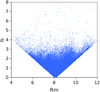 |
Fig. C.1. Orbital planar amplitude a (kpc) in terms of the orbital mean radius rm (kpc), whose average value is rc = 8.3 kpc. |
In the interval [rc − δ, rc + δ], the constant 2B in Eq. (13) can be estimated as

Therefore, we assume
where ξ is an intermediate radius satisfying ν(ξ) ≥ ν(rc) and ν(ξ)→ν(rc) when δ → 0.
A maximum amplitude δ around rc corresponds to a maximum planar eccentricity ε satisfying δ = rc ε. Thus,
We now define the following function, which is a slight modification of Eq. (13),
Around the local circular velocity point, rc = r0, we consider the value ν(ξ) as an average value, valid for all the stars in the subsample, so that, according to Eq. (C.1), the function f can also be expressed as

Now, we analyse the change of slope,  , by writing the last term depending on the vertical eccentricity
  , as
, as
![$$ \begin{aligned} f_\varepsilon (z_{\rm max},r_{\rm m}) = z^2_{\rm max} \left[ \frac{\kappa ^2}{4} + \left(\nu ^2(\xi )-\frac{\kappa ^2}{4} \right) \frac{r_0^2}{r_{\rm m}^2} (1-\varepsilon ^2)^2 \; \frac{1}{1+C {e^{\prime 2}}} \right]. \end{aligned} $$](/articles/aa/full_html/2021/08/aa40835-21/aa40835-21-eq113.gif)
For a small δ, since r0 − δ ≤ rm ≤ r0 + δ, in average, for the subsample we may approximate  . In this way, it is possible to justify that the slope q decreases with e′ for fixed ε, and, similarly, the slope decreases with ε2 for fixed e′. Thus, for subsamples containing stars with increasing planar eccentricity we will get curves that, in average, have lower slope.
Therefore, the function fε defined in Eq. (C.3) is a decreasing function of the non-negative value ε2, which satisfies:

Then, we may adjust the parameters of the MVC by determining the upper limit of the points plotted from the function f (Fig. C.2, right) instead of by using the curve w2(zmax, rm) (Fig. C.2, left).
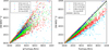 |
Fig. C.2. Squared maximum vertical peculiar velocity (W − W0)2 (km2 s−2) compared to those predicted by w2(zmax, rm) (left) and by f(zmax, rm) (right). The colours indicate different planar eccentricities. |
The fitting of this curve, by assuming r0 = 8.3, and using the estimates from Paper I, ν(r0) = 63 km s−1 kpc−1 and κ = 37 km s−1 kpc−1, provides the value C = 21 ± 1, which is used to plot the MVC in Fig. 9.
Appendix D: Local potential
With the local constants M, A, B, and C already evaluated, we may estimate the local approximation of the potential given by Eqs. (2) and (8). It is interesting to focus on the non-harmonic part 𝒰0. The harmonic part produces a trivial attractive force for M > 0. For the actual constants, in particular C = 21, the level curves for the total potential 𝒰 and the term 𝒰0 are displayed in Fig. D.1.
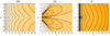 |
Fig. D.1. Level curves for the potential 𝒰(r, z), together with the contributed terms 𝒰0 and 𝒰z, for the actual value C = 21. |
There is a critical value for C that determines qualitatively the shape of the potential. In the actual case A < 0 and B > 0. If we define  , we may write Eq. (8) as
According to our working sample, the limiting value is C0 ≈ 11, which is lower than the actual value for C.
Although it goes beyond the scope of this paper, it is easy to see that the sign of the force in the radial direction associated with 𝒰0 depends on the sign of C − C0. If C − C0 ≥ 0, as in the actual case, being A < 0, this force is always attractive. On the other hand, if C − C0 < 0, this force would have opposite signs depending on the region of the Galaxy. To make a comparison with Fig. D.1, we show in Fig. D.2 the contour plots for the critical case and a case with C < C0.
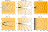 |
Fig. D.2. Contour plots for the terms 𝒰0, 𝒰z and the potential 𝒰 for the critical case C = 11 (top) compared to a case with C = 6 (bottom). |
The case C = C0 is equivalent to  . This expression was studied in Cubarsi et al. (2017) and could not fit to the actual MVC.
It is also illustrative to write the potential by separating the spherical part 𝒰R, depending on R2 = r2 + z2, and the remaining part 𝒰z, which is proportional to z2. Then, we may write the potential as 𝒰 = 𝒰R + 𝒰z with
The level curves for 𝒰z are also displayed in Fig. D.1. In all the cases, far from the origin, the potential is approximately spherical, due to the harmonic term. The non-harmonic term 𝒰0 is the one providing the general features of 𝒰, specially close to the origin. On the other hand, the contribution of the term 𝒰z is regulated by the constant C.
Appendix E: Average slope
With regard to Fig. 10, we aim to prove that the intersection of the curve w2 = g(e′2) and the horizontal line  determines the straight line w2 = p0 e′2 passing through the origin, whose slope is the geometrical mean (grey-dashed line in Fig. 10) of the slopes of both limiting tangents, namely:

Firstly, we explicitly write the abscissa of the intersection  . According to Eqs. (23) and (26), we have
Now we prove that the straight line  , at
, at  takes the value
  . Thus, according to Eqs. (26) and (E.1), we have
Therefore, in the range of  , the disc and halo coexist, although the former, with lower eccentricity stars, is obviously prevailing. Within this range, in the angular region of Fig. 10 where the slope p = w2/e′2 takes values
  , the stiffness decreases as increasing the vertical eccentricity.
In the range of  (mostly corresponding to halo stars), in the angular region where p = w2/e′2 takes values
  , the stiffness remains nearly constant.
We calculate the slope of the velocity curve at the limiting point  . The derivative of Eq. (23) is
At  , according to Eq. (E.1), by simplifying, we get
  . For the actual estimates, in the range
  , g′(e′2) drops 86%, while in the range 0 ≤ e′2 ≤ 1, g′(e′2) drops 90%. Then, it is justified to affirm that from
  onward the slope is nearly constant.
Appendix F: Local density
In cylindrical coordinates, by assuming axial symmetry, Poisson’s equation gives the expression
The gravitational constant is G = 4.301 × 10⁻⁶ km2 s−2 kpc  .
.
For the potential in Eq. (2), we calculate the following potential derivatives in terms of F(s), bearing in mind that  :
:
Thus, together with Eq. (B.2), we can write Poisson’s equation as

By applying a substitution for F(s), from Eq. (8), namely,  and
and  , in the foregoing expression, we get

If we plot the local density ρ0(z) ≡ ρ(r0, z) (Fig. F.1, left panel), we observe that for C = 21 there is a local minimum of ρ0(z), approximately with vanishing density, which would determine the maximum height z0 of the disc by producing a clear separation of the disc and halo components. For higher values of C, the density of this minimum would be negative (green dashed line), which would make no sense. Instead, for lower values of C, the disc and halo components would virtually overlap (green dashed line), also by producing a relative minimum of density.
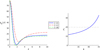 |
Fig. F.1. Density ρ(r0, z) = ρ0(z) (×106 M⊙ kpc−3) in terms of z (kpc) for C = 21 (blue), compared to other values of C (left). Minimum value for C required to produce a non-negative density, in terms of κ (right). |
We calculate the abscissa z0 of this minimum. The density derivative is
The local minimum for r = r0 must satisfy  , from where, by assuming
  , we have
It is interesting to point out two approximations of the above equation. Firstly, we consider a more coarse approximation. If  , we may consider
  , which is within the error range obtained for this constant. It yields

Such an estimation matches the expression for z0 in Eq. (25), derived from the analysis of the MVC.
Secondly, we consider a more accurate one. We may assume  . Then,
  . Therefore,
In Fig. 13 (left), we may observe that both are good approximations.
Now, we determine the minimum value of C that guarantees a non-negative density from the equation ρ(r0, z0(C)) = 0. The value of C is especially dependent on M, which is a function of κ alone. Then, by assuming fixed values for ν and γc, such a relationship implies that the minimum C and κ are mutually dependent, as shown in Fig. 13 (right panel). The critical value can be expressed analytically in terms of M, A, and B, by using the approximation of Eq. (F.4), as

It so happens that the value C ≈ 21 we estimated is higher than the minimum values derived for the thin and thick discs. However, the value κ ≈ 41 km s−1 kpc−1 obtained for the whole working sample selected as |W|≤170 km s−1 in Paper I, is fully consistent with such a critical value C ≈ 21. Therefore, in order to estimate some properties of the local stellar density of the disc, we adopt this approximated model, where the local minimum of vanishing density takes place at the point z0. Even though such a model implies that there is no overlapping between disc and halo, which seems unrealistic, it is a simple way to obtain an alternative measurement of the maximum height of the disc.
All Tables
Parameters delimiting the triangular regions Ri according to the stars’ orbital parameters.
Mean velocities, central moments, and population fractions (relative to the whole sample) from the eccentricity diagram.
All Figures
|
Fig. 1. Maximum height zmax (kpc) in terms of the vertical heliocentric velocity W (km s−1), with the biquadratic fit of Paper I (discontinuous line). The distance to the local radius is indicated in the colours. |
| In the text | |
|
Fig. 2. Squared vertical peculiar velocity (W − W0)2 (km2 s−2) at the GP in terms of (left) the squared maximum height, |
| In the text | |
|
Fig. 3. Duffing potentials (left) with B > 0 (red) and B < 0 (blue) compared to the harmonic potential (grey). Maximum velocity curves (right) associated with these potentials. |
| In the text | |
|
Fig. 4. Quarter ellipses (left) defining the regions R2 (closer to the origin) and R4 (farther from the origin), according to the biquadratic fit (continuous green curves), potential model (continuous blue curves), and epicycle approach (dotted red curves). The dotted green and blue curves are the respective approximations from quarter ellipses. The same regions in terms of the squared eccentricities are displayed on the right. |
| In the text | |
|
Fig. 5. Triangular regions according to Table 1, for the current potential model (left) and for the biquadratic approximation (right). The complementary area is the halo (red). |
| In the text | |
|
Fig. 6. Strömberg’s law and asymmetric drift equation adjusted for several subsamples. Top: Strömberg’s law for thin disc subsamples (black dots) accounting for the total velocity dispersion σ2 (km2 s−2) and the velocity moment μ200 (km2 s−2) in terms of their heliocentric rotation velocity V0 (km s−1). Fitting of Eq. (21) (right panel) for thin disc subsamples (red dots) using the optimal value of γc. Bottom: (left panel) Strömberg’s law for the total thin disc (t, red line) and the thick disc (T, black line) subsamples; and (right panel) for thin disc, thick disc, and halo (H) components. |
| In the text | |
|
Fig. 7. Triangular regions R1 to R4 for the actual eccentricities (as depicted in Fig. 5) obtained from Eq. (18) (left), and exact regions (right) obtained from Eq. (17). |
| In the text | |
|
Fig. 8. Regions R1 to R4 according to the eccentricities obtained from Eqs. (12) and (15), in terms of the star’s velocities. |
| In the text | |
|
Fig. 9. Squared vertical peculiar velocity (W − W0)2 (km2 s−2) at the GP in terms of (left) the squared maximum height |
| In the text | |
|
Fig. 10. Contribution of the disc and halo components to the maximum velocity curve, i.e., local vertical peculiar velocity w = W − W0 (squared, km2 s−2) at the GP in terms of vertical eccentricity e′ (squared, dimensionless). The continuous lines correspond to the whole curve (black), the disc term (blue), and the halo term (red). The dashed blue and red lines are the respective tangent (TD) and asymptote (TH), the dashed grey line is their geometric mean, and the dashed green line marks the bound for the vertical speed (squared) of disc stars. |
| In the text | |
|
Fig. 11. Maximum height zmax (kpc) in terms of the vertical heliocentric velocity W (km s−1) according to different approaches: continuous black line for the model provided by the local potential, discontinuous red line for the biquadratic fit of Paper I, and discontinuous grey line for the disc component alone. |
| In the text | |
|
Fig. 12. Density ρ(r0, z) = ρ0(z) (×106 M⊙ kpc−3) in terms of z (kpc) for C = 21 (blue), compared to other values of C. |
| In the text | |
|
Fig. 13. Maximum height (left) z0 (kpc) in terms of C (blue curve) from Eq. (F.3), compared to the approximations from Eq. (F.4) (green, similar to Eq. (25)) and Eq. (F.5) (red). Maximum vertical peculiar velocity (right) of disc stars w0 (km s−1) from Eq. (26). The dashed grey lines mark the estimated values, z0 = 1.8 kpc and w0 = 115 km s−1, for C = 21. |
| In the text | |
|
Fig. 14. Function D0(z0) (×106 M⊙ kpc−2) plotted in terms of C and z0 (left and central panels). The dashed grey lines mark the estimated values for C = 21 and z0 = 1.8 kpc. Fraction of stars with |z|≤z0 relative to the number of stars with |z|=z0 is given in the right panel. |
| In the text | |
|
Fig. 15. Relative decrease of density in the local cylinder in the range [ − z, z] (kpc), when comparing a disc model with velocity limit w0 = 115 km s−1 (z0 = 1.8 kpc) to another one with w0 = 135 km s−1 (z0 = 2.1 kpc). |
| In the text | |
|
Fig. C.1. Orbital planar amplitude a (kpc) in terms of the orbital mean radius rm (kpc), whose average value is rc = 8.3 kpc. |
| In the text | |
|
Fig. C.2. Squared maximum vertical peculiar velocity (W − W0)2 (km2 s−2) compared to those predicted by w2(zmax, rm) (left) and by f(zmax, rm) (right). The colours indicate different planar eccentricities. |
| In the text | |
|
Fig. D.1. Level curves for the potential 𝒰(r, z), together with the contributed terms 𝒰0 and 𝒰z, for the actual value C = 21. |
| In the text | |
|
Fig. D.2. Contour plots for the terms 𝒰0, 𝒰z and the potential 𝒰 for the critical case C = 11 (top) compared to a case with C = 6 (bottom). |
| In the text | |
|
Fig. F.1. Density ρ(r0, z) = ρ0(z) (×106 M⊙ kpc−3) in terms of z (kpc) for C = 21 (blue), compared to other values of C (left). Minimum value for C required to produce a non-negative density, in terms of κ (right). |
| In the text | |
Current usage metrics show cumulative count of Article Views (full-text article views including HTML views, PDF and ePub downloads, according to the available data) and Abstracts Views on Vision4Press platform.
Data correspond to usage on the plateform after 2015. The current usage metrics is available 48-96 hours after online publication and is updated daily on week days.
Initial download of the metrics may take a while.