| Issue |
A&A
Volume 652, August 2021
|
|
|---|---|---|
| Article Number | A143 | |
| Number of page(s) | 10 | |
| Section | The Sun and the Heliosphere | |
| DOI | https://doi.org/10.1051/0004-6361/202140374 | |
| Published online | 25 August 2021 | |
A deep learning method to estimate magnetic fields in solar active regions from photospheric continuum images⋆
1
Key Laboratory of Solar Activity, National Astronomical Observatories, Chinese Academy of Sciences, 20 Datun Road, Beijing 100101, PR China
2
School of Astronomy and Space Science, University of Chinese Academy of Sciences, No. 19(A) Yuquan Road, Beijing 100049, PR China
3
Yunnan Observatories, Chinese Academy of Sciences, Kunming, 650011 Yunnan, PR China
e-mail: jkf@ynao.ac.cn
4
School of Space and Environment, Beihang University, Beijing, PR China
5
College of Computer Science, Sichuan University, Chengdu 610065, PR China
6
Big Bear Solar Observatory, New Jersey Institute of Technology, Big Bear City, CA 92314-9672, USA
Received:
19
January
2021
Accepted:
5
June
2021
Context. The magnetic field is the underlying cause of solar activities. Spectropolarimetric Stokes inversions have been routinely used to extract the vector magnetic field from observations for about 40 years. In contrast, the photospheric continuum images have an observational history of more than 100 years.
Aims. We suggest a new method to quickly estimate the unsigned radial component of the magnetic field, |Br|, and the transverse field, Bt, just from photospheric continuum images (I) using deep convolutional neural networks (CNN).
Methods. Two independent models, that is, I versus |Br| and I versus Bt, are trained by the CNN with a residual architecture. A total of 7800 sets of data (I, Br and Bt) covering 17 active region patches from 2011 to 2015 from the Helioseismic and Magnetic Imager are used to train and validate the models.
Results. The CNN models can successfully estimate |Br| as well as Bt maps in sunspot umbra, penumbra, pore, and strong network regions based on the evaluation of four active regions (test datasets). From a series of continuum images, we can also detect the emergence of a transverse magnetic field quantitatively with the trained CNN model. The three-day evolution of the averaged value of the estimated |Br| and Bt from continuum images follows that from Stokes inversions well. Furthermore, our models can reproduce the nonlinear relationships between I and |Br| as well as Bt, explaining why we can estimate these relationships just from continuum images.
Conclusions. Our method provides an effective way to quickly estimate |Br| and Bt maps from photospheric continuum images. The method can be applied to the reconstruction of the historical magnetic fields and to future observations for providing the quick look data of the magnetic fields.
Key words: Sun: magnetic fields / Sun: photosphere / methods: statistical
Movie is available at https://www.aanda.org
© ESO 2021
1. Introduction
The magnetic field is the underlying cause of solar activities. The strength of the magnetic field has strong correlations with the solar cycle and irradiance variability. Therefore the magnetic field is generally considered as the most important physical parameter and holds a central position in solar physics (Solanki et al. 2006).
The measurement of the photospheric magnetic field relies on remote sensing data by means of the Zeeman effect. George Ellery Hale was the first person who found a strong magnetic field in a sunspot based on the triplet splitting of the photospheric spectral lines. Later, Babcock (1953) developed a magnetograph that can measure the circular polarization and weak photospheric magnetic fields. Severny (1964) invented a vector magnetograph, which has the ability to obtain the total polarization information, that is, Stokes I, Q, U, and V profiles of a magnetic sensitive line. After obtaining the Stokes profiles, the vector magnetic field (longitudinal and transverse magnetic fields as well as the azimuth angle) is then derived using the Stokes inversion technique, which minimizes the observed and synthetic profiles calculated from polarized radiative transfer theory. So far, analytical and numerical solutions are generally employed for synthetic Stokes profiles (de la Cruz Rodríguez & van Noort 2017; Li et al. 2019; Lagg et al. 2017; Iglesias & Feller 2019; Bai et al. 2013, 2014). Since 2000 the machine learning method has also been employed to derive vector magnetic field from Stokes parameters (Rees et al. 2000; Socas-Navarro 2003; Asensio Ramos & Díaz Baso 2019; Guo et al. 2020; Liu et al. 2020).
In addition to the methods mentioned above, we can also use indirect manifestation to estimate the photospheric magnetic field, such as the relatively dark parts in the sunspots, enhanced emission in chromosphere, and the corona in network magnetic field regions. Chatzistergos et al. (2019) recovered the unsigned longitudinal photospheric magnetic field from Ca II K observations based on the statistical relation between magnetic field strength and Ca II K core brightness. Similar studies have also been carried out by Virtanen et al. (2019). With a machine learning method, Kim et al. (2019) tried to construct far-side longitudinal magnetograms from the Extreme UltraViolet Imager (EUVI) 304 Å images on board the Solar Terrestrial Relations Observatory (STEREO) with the trained model of the longitudinal magnetograms from the Helioseismic and Magnetic Imager (HMI) on board the Solar Dynamics Observatory (SDO) and the EUVI images using conditional generative adversarial networks (cGANS). Combining front-side longitudinal magnetograms from HMI with far-side longitudinal magnetograms from the STEREO EUV observations by the deep learning model, Jeong et al. (2020) made global magnetic field synchronic maps. Discussion regarding the reliability of AI generated magnetograms just from EUV images are available in Liu et al. (2021) and Park et al. (2021). Shin et al. (2020) also generated longitudinal magnetic fields with polarities from Ca II K observations using novel deep learning models based on cGAN.
In the paper, we propose a new machine learning method to estimate the photospheric magnetic fields from the corresponding continuum images. Our estimated magnetic fields include both the radial and transverse components. This is distinct from current reconstruction models (Chatzistergos et al. 2019; Kim et al. 2019; Shin et al. 2020; Jeong et al. 2020), which only consider the radial or line-of-sight component of the solar magnetic fields. The transverse magnetic field is very important in the understanding of solar activity, for example, the variations of the transverse magnetic field during solar flares (Wang et al. 2002; Song & Zhang 2016; Su et al. 2011; Wang & Liu 2015).
The paper is organized as follows. We present the data and the machine learning method in Sect. 2. In Sect. 3, the results are presented and their reliability is evaluated by comparisons of radial and transverse photospheric magnetic fields from the Stokes inversion and machine learning methods. Section 4 summarizes our conclusions.
2. Data and machine learning method
We use Space-weather HMI active region patches (SHARPs) data (Hoeksema et al. 2014). The data are in a heliographic cylindrical equal-area (CEA) coordinate system with the cadence of 720 s. In the data, the projection effect is corrected. Furthermore, the vector field B is transformed into the components Br, Bθ, and Bϕ in standard heliographic spherical coordinates. In the paper, four kinds of images, that is, the continuum (I), Br, Bθ, and Bϕ images are used in the preprocessing step. The continuum images are calculated by fitting the full Stokes profiles of the Fe I 617.3 nm magnetic sensitive line computed from the integrated observation of 12 min (Hoeksema et al. 2014). In this work we only consider the unsigned radial component of the magnetic field, |Br|. The other two components, Bθ and Bϕ are combined to create the transverse field, Bt, according to the following formula:
We built two independent models to estimate |Br| and Bt from the corresponding continuum images. For the training dataset, its input is the continuum image, which is normalized by its mean value. The outputs for the two models are |Br| and Bt, respectively. A total of 7890 groups of data covering 17 SHARPs from 2011 to 2015 (see Table 1) are used to construct the model. Two criteria are employed to select the dataset. One criterion is that the number of rows in the SHARP data should be larger than 200 pixels, covering a large field of view. The other criterion is that the SHARP data within the range of ±65° from disk center are used. We randomly selected 15% of the whole dataset as the validation data and the remaining 85% are used for the training data. The trained model, test code, and the result of the test datasets (five SHARP numbers) are publicly available1.
Detailed information of the training and validation datasets.
Each model is constructed by a deep convolution neural network (CNN) with a residual architecture (He et al. 2015), which is a wide adopted algorithm of machine learning. The initial layers and residual group of the network extract features from the input photospheric continuum image, while the final convolutional layers predict the corresponding magnetic field (|Br| or Bt). The full network is shown in Fig. 1, where different colored cubes represent different layers. The initial layer is a convolutional layer, and its outputs serve as inputs to the residual blocks for further deep residual learning. Ten residual blocks are stacked, and each block contains a residual channel with a single shortcut connection. The residual block is essentially made up of two weight-shared convolution layers, each followed by a batch normalization layer and ReLU activation with a skip connection to before the last ReLU activation. Each convolutional layer has 256 kernels of 3 × 3 and keeps the size of each feature map fixed by one stride and zero padding. In the last layer, the network ends with a 3 × 3 convolutional layer to reconstruct the magnetic field image. Finally, the goal of the training model is to minimize the loss function, which is the mean squares error (MSE) and is defined by Eq. (2) as
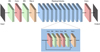 |
Fig. 1. Architecture of the deep neural network used in the paper. |
where IMAGEinv represents either |Br| or Bt from SHARP data, IMAGECNN is the image from the trained model, and N is the pixel numbers. Our model is trained by the Adam optimizer with the default setting for the configuration parameters, that is, α = 0.001, β1 = 0.9, β2 = 0.999, and ϵ = 10−8. We also tried to generate Br. The CNN model is not converged if Br with polarity is investigated. Therefore, we use only |Br| other than Br in the following.
3. Results and comprehensive evaluations of the models
SHARP No. 2875 observed from June 18 to June 21, 2013 covers the evolution of the active region (AR) from small pores to a complex sunspot group. Hence we take it as a representative of the test dataset and present comprehensive comparisons of the magnetic field between the inversion and CNN model in Sect. 3.1. We then give overall comparisons of the other three ARs in Sect. 3.2.
3.1. SHARPS No. 2875 as a representative of the test dataset
From the continuum image in Fig. 2a, we can see a pore in region R1 surrounded by several mini-pores. The corresponding Br − inv, |Br − inv|, and Bt − inv from Stokes inversions are shown in Figs. 2b–d, respectively. The |Br − CNN| and Bt − CNN from the trained CNN models are shown in Figs. 2e and f, respectively. This shows that we can estimate the |Br| and Bt not only for the pore regions but also for the strong network regions (Region R2). The correlation coefficient (CC) between |Br − inv| and |Br − CNN| is 0.90, while the CC for Bt is 0.82. Figure 2g is the difference map between |Br − inv| and |Br − CNN|, while that of Bt is represented in Fig. 2h. The difference maps show a nonuniform pattern owing to the diverse accuracy of the estimated magnetic fields for various solar features. The values at the pore or strong network region are the lowest, while those at the weak network regions are the largest. The mean and standard deviation values of the difference maps are 4.3 G and 37.1 G for the |Br|, while the corresponding values for the Bt are 15.3 and 35.1 G. The results for the other times can be found in the online movie. The last row in Fig. 2 is the scatter plots of |Br − inv| versus |Br − CNN| (Fig. 2i) and Bt − inv versus Bt − CNN (Fig. 2j). We carried out linear fittings of the scatter plots. The regions with |Br − inv| greater than 30 G and Bt − inv greater than 100 G are used for the fitting. The final results are |Br − CNN|= − 5.78 + 0.89 × |Br − inv|, Bt − CNN = −13.1 + 0.95 × Bt − inv, respectively. The estimated values of |Br − CNN| and Bt − CNN are slightly lower than those from Stokes inversions.
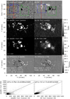 |
Fig. 2. Result from SHARP No. 2875. Panels a–d: image of continuum, Br, |Br|, and Bt from Stokes inversion, respectively. Panels e and f: |Br| and Bt estimated from panel a with the trained CNN model. Panel g is the difference map of |Br| between Stokes inversion and the CNN model, while panel h is that of Bt. Panels i and j: scatter plots of |Br| and Bt between the two methods. Regions R1 and R3 indicate the region used in Fig. 3. Region R2 and red line L1 are used in Fig. 4. An associated animation of these panels is available online. |
Figures 3a–g illustrate the evolution of the photospheric continuum images in Region R1 in Fig. 2a from 13:12 to 16:48 UT with a cadence of 36 min. At 13:12 UT, there are two pores with opposite polarities denoted as N1 and P1. Later, the distance between N1 and P1 becomes larger and some filament-like (or elongate dark) structures occur between them (see the ellipse E1 region), indicating the scenario of the emergence of bipolar magnetic regions. The evolution of Br from the Stokes inversion (the second column in Fig. 3) confirms the flux emergence process. From the evolution of Bt (see E1 region in the fifth column), it also clearly shows the emergence of the transverse magnetic field between the two pores. The filament-like structures seen in the continuum images mainly represent the transverse magnetic field with negligible Br. With the help of photospheric continuum images and our trained CNN model, we derived the |Br − CNN| map (the third column) and the transverse magnetic field Bt − CNN map (the sixth column). The morphology of |Br| and Bt maps between the two methods is very similar. The CCs for |Br| are all above 0.95 for the seven images, while those for Bt are between 0.91 and 0.95. From the distribution of the scatter plots of |Br − inv| versus |Br − CNN| (the fourth column) and Bt − inv versus Bt − CNN (the seventh column), it is found that they are all near the diagonal line, indicating that the estimated values from the CNN method are consistent with those from Stokes inversions. It is worth mentioning that the emergence of the transverse magnetic field Bt is estimated well quantitatively from the filament structures with a mean systematic difference about 30 G.
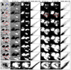 |
Fig. 3. Evolution of the Region R1 in Fig. 2a from 13:12 to 17:24 UT (panels a–g). The columns from left to right are, in order, the continuum images, Br from Stokes inversion, |Br| from CNN model, scatter plots of |Br| between the two methods, Bt from Stokes inversion and CNN model, and scatter plots of the two methods, respectively. The elliptical E1 indicates the region where the transverse magnetic field emerges. Panel h: values for a sunspot from R3 region but for a different time. |
In addition to the bipolar regions with magnetic field emergence, we further show the estimated magnetic fields for a sunspot region (R3 region at 05:00 UT on June 21) containing both umbra and penumbra. The result is indicated in the last row of Fig. 3. The CCs between the two methods are 0.97 and 0.93 for the |Br| and Bt, respectively. The distributions of the scatter plots of |Br − inv| versus |Br − CNN| (the fourth column) and Bt − inv versus Bt − CNN (the seventh column) are both near the diagonal line, indicating that the values are very similar. Generally, the value of |Br| is higher while that for Bt is lower in the center of umbra than the nearby regions. Our reproduced |Br| and Bt maps are consistent with the scenario.
To better verify the estimated |Br| and Bt maps from the photospheric continuum images with our trained CNN model, we further calculate the evolution of |Br| and Bt for SHARP No. 2875 within three days and compare these values with those from the Stokes inversion method. Figure 4a shows the comparison of the temporal evolution of the averaged |Br| between the values from the CNN model and those from the Stokes inversion method during three days. The two plots closely follow each other. They both show a gradually increase in values due to the magnetic emergence and some small-scale variations. The CC of the two curves is 0.997. Figure 4b shows the comparison of the averaged Bt during the same time period as Fig. 4a. Although the result of averaged Bt from the inversion shows several small-scale fluctuations, our CNN model successfully reproduced these values, with a CC of 0.994. Except for the high correlations, it is found that the estimated values of |Br| and Bt from our CNN model are systematically underestimated. After employing a simple linear fitting, we can correct the systematic bias. The corrected plots are shown in Figs. 4a and b with orange lines.
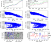 |
Fig. 4. Evolution of the averaged |Br| (panel a) and Bt (panel b) for SHARP number 2875 within about three days. Panels c and d: scatter plots of the continuum brightness in Fig. 3h vs. the |Br| from Stokes inversion and CNN model methods, respectively. The one between the continuum brightness and Bt is shown in panels e and f. The left and right images in panel g being Region R2 in Fig. 2a are the same with the exception that the left part is overplotted with the contour of Br. The contour levels are 45 and 200 G. The green ellipse E2 denotes the strong network region. Panel h: value of the continuum image extracted from the red line L1 in Fig. 2a, while the blue line represents the corresponding Br value. |
We ask why we can estimate |Br| and Bt maps just from photospheric continuum images. For the Stokes inversion method, at least four parameters are needed, that is, the Stoke I, Q, U, V maps from a magnetic sensitive line to derive Br, Bt, and the azimuth angle (de la Cruz Rodríguez & van Noort 2017; Li et al. 2019). The derived accuracy can further be improved if we employ more spectral points. At this point, we would like to emphasize that the Stokes inversion is done pixel by pixel and does not consider the spatial relationship between adjacent pixels. For the CNN models, we consider the spatial correlation of the images with all kinds of solar features from the training datasets so that the nonlinear relationships between I and |Br| as well as Bt can be derived. In other words, the reason behind the effectiveness of our method is the statistical spatial correlations of I versus |Br| and I versus Bt identified by the CNN algorithm.
Figure 4c shows the relationship between I and |Br − inv| from the Stokes inversion, while that of I and |Br − CNN| from the CNN model is presented in Fig. 4d. The relations for the I versus Bt − inv and I versus Bt − CNN are shown in Figs. 4e and f, respectively. The results are based on the sunspot region presented in Fig. 3h including both umbra and penumbra. We see that with the decrease of the continuum intensity, the strength of |Br − CNN| from the CNN model increases, which is a well-known property. The CC value between I − |Br − CNN| and I − |Br − inv| is 0.97. The well-reproduced I − |Br| relation by the CNN models illustrates how well the |Br| map can be reproduced based on the continuum images.
Because it is different from the monotonic relation between |Br| and I, the relation between Bt and I from the inversion (Bt − inv, Fig. 4e) and CNN model (Bt − CNN; Fig. 4f) shows a crocodile-mouth-type shape with three branches. The upper branch shows the decrease of I with the increase in Bt, which is similar to the I − |Br| relation. The lower branch shows an opposite trend. The intensity I increases with the increase in Bt. Both the simulations (Rempel 2012) and data analysis (Mathew et al. 2004; Borrero & Ichimoto 2011; Song & Zhang 2016; Sobotka & Rezaei 2017) show that Bt is larger with the increasing continuum intensity in the umbra and umbra-penumbra boundary region and then has the opposite tendency in the outer penumbra regions. The Bt property of umbra and penumbra contributes to the upper and lower branches. There is no significant relationship between I and Bt in the middle branch when Bt is weaker than 700 G. The result from the CCN model well reproduces the three branches (crocodile-mouth-type shape). This verifies the effectiveness of the CCN model to reconstruct the transverse field maps from the continuum images.
Usually, the strong network region is located at the boundary of supergranulation so we can see more small-scale and blurred structures with less contrast relative to the nearby granulations without magnetic fields, especially in the low-resolution data (Kobel et al. 2012; Criscuoli 2013; Kahil et al. 2019). The scenario can be found in Figs. 4g and h. The green ellipse E2 in Fig. 4g indicates the strong network region. It has blurred patterns relative to the nearby regions. The blue and red lines in Fig. 4h represent the corresponding Br and I values, respectively, which are extracted from the red line L1 in Fig. 2a. For the network regions between the two green vertical dot-dashed lines (the red line inside the green ellipse E2), the continuum intensity with stronger magnetic field strength shows less contrast.
3.2. Overall comparisons of the other three ARs
In the above subsection, we showed the estimated magnetic fields from series continuum images of an AR. In this subsection, we illustrate the results for the other three ARs in different years. Only one continuum image is presented for each AR. Figure 5 shows the result for SHARP No. 26, which is observed on May 21, 2010. We can see the leading and the following sunspots from the continuum image. The corresponding |Br − CNN| and Bt − CNN maps estimated from the continuum image with our trained CNN model are represented in Figs. 5d and e, respectively. The CC between |Br − inv| and |Br − CNN| is 0.95, while that for Bt is 0.91. Figure 5f is the |Br| difference map between the two methods, while that of Bt is shown in Fig. 5g. The difference maps also have nonuniform patterns owing to the diverse accuracy of the estimated magnetic fields for various solar features. The mean and standard deviation values of the difference map for the |Br| are −2 G and 85.3 G, while the corresponding values for the Bt are −12 G and 73 G. The linear fittings of |Br| and Bt between the two methods are carried out. The final results are |Br − CNN| = 1.2 + 0.98 × |Br − inv| and Bt − CNN = 35.19 + 0.83 × Bt − inv.
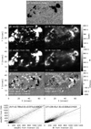 |
Fig. 5. Result from SHARP No. 26. Panels a–c: image of continuum, |Br|, and Bt from Stokes inversion, respectively. The unsigned Br and Bt estimated from panel a with our CNN model are shown in panels d and e. Panel f is the difference map of |Br| between Stokes inversion and CNN model, while panel g is that of Bt. Panels h and j: scatter plots of |Br| and Bt between the two methods. |
We illustrate the estimated |Br − CNN| and Bt − CNN for SHARP No. 4375 observed on July 19, 2014 in Fig. 6. It also consists of the leading and the following sunspots, as seen from the continuum image in Fig. 6a. The other panels are arranged in the same order as Fig. 5. The CC of |Br| between the Stokes inversion and the CNN methods is 0.96, while the value for Bt is 0.94. Regarding the mean and standard deviation values of the difference map, they are 5 G and 87 G for |Br| as well as 0.7 G and 64 G for Bt, respectively. The linear fitting of the scatter plots in Figs. 6h and i are |Br − CNN|= − 0.6 + 0.95 × |Br − inv| and Bt − CNN = −21.9 + 1.01 × Bt − inv.
The last test dataset is from SHARP No. 5118 observed on Jan. 26, 2015 and its comparison results are shown in Fig. 7. SHARP No. 5118 is the bipolar sunspots again. The CCs of |Br| and Bt between the two methods are 0.95 and 0.94, respectively. The mean and stand deviation values of the difference map are 6 G and 84 G for |Br|. The values for Bt are −3 G and 69 G, respectively. We get |Br − CNN|= − 5.68 + 0.96 × |Br − inv|, and Bt − CNN = 19.66 + 0.92 × Bt − inv after employing the linear fittings of the scatter plots.
The above results further demonstrate that our CNN method has the ability to estimate both the |Br| and Bt maps just from the continuum image for the sunspot region. From the comparison of panels a and b in Figs. 5–7, the regions with lower values in the continuum image have larger |Br|. Our estimated |Br − CNN| value is higher in the umbra center, which is consistent with the well-known I − |Br| relationship. Regarding the one between I and Bt, the strength of Bt firstly increases with the decreasing intensity for the outer penumbra region. Then a reverse trend is found in the umbra and umbra-penumbra boundary region as seen from Fig. 4e. Therefore the Bt map is dark in the center of the umbra. Our estimated Bt − CNN can also recover the above relationship from the comparison of panels a and e in Figs. 5–7.
4. Conclusions and discussion
In the paper, we have suggested a method to reproduce the photospheric unsigned radial field |Br| and the transverse field Bt for the ARs utilizing the corresponding continuum images by a deep convolutional network with a residual architecture. We use the Stokes inversion result to train our model. Our purpose is not to replace the Stokes inversion method, which is generally regarded as an accurate and robust method. Our method provides an alternative tool to quickly reconstruct |Br| and Bt maps for the solar irradiance and flare-related research. Our models can especially be applied to future solar instrumental projects for providing the quick look maps of |Br| and Bt with observed continuum images since the computing time spent on spectropolarimetric inversions is very large. The main conclusions can be summarized in the following:
-
From the photospheric continuum image, we can estimate the photospheric |Br| map for the strong network, pore, and sunspot (penumbra and umbra) regions. More importantly, the transverse magnetogram is also obtained in the sunspot regions. The values of the estimated |Br| and Bt are slightly less (in the range of 3%−10%) than those from Stokes inversion method, as seen from the last row of Figs. 2, 5–7. The evolution of the averaged |Br| and Bt for the SHARP No. 2875 from our trained CNN model follows well that from Stokes inversion method for both the large- and small-scale fluctuations, verifying the consistency and stability of the CNN model. The estimated |Br − CNN| and Bt − CNN maps for the other three ARs observed at different years also agree well with those from Stokes inversion method.
-
From series of continuum images, we can even detect the emergence of transverse magnetic fields (filament-like pattern) quantitatively with the trained CNN model. The powerful studying and generalizing ability of the CNN model can reproduce the complicated nonlinear relationship between the continuum intensity versus the |Br| and the Bt. That is possibly the reason we can estimate the magnetic fields just from photospheric continuum images.
The relationship between the magnetic field strength and photospheric continuum brightness is obvious in the sunspot; thus the method proposed in the paper can be applied to estimate |Br| and Bt maps based on 100 years of photospheric continuum images for the ARs. However, the relationship of I − |Br| and I − Bt is very weak for the network regions (Kobel et al. 2012). From the online movie, some brightness scintillation is found in the continuum image possibly related to the p-mode oscillation, resulting oscillations in the estimated |Br| and Bt with the CNN model. We will try to remove them and check if it is possible to estimate the weak magnetic fields in the network regions in the following work. Moreover, we would like to train the model combining the three-dimensional magnetohydrodynamics simulation data with very high spatial resolution (Cheung & Isobe 2014). This may provide an alternative way to diagnose the fast evolution of transverse magnetic fields during small-scale and short-lived solar activities, which are found by the ground-based high-resolution telescopes and are very difficult to derive because it takes a long time to carry out Stokes observations and inversions (Bai et al. 2019; Louis et al. 2015; Lim et al. 2011; Yang et al. 2019).
Movie
Movie 1 associated with Fig. 2 (figure2_movie) Access here
Acknowledgments
We thank Dr. Yongliang Song for helpful discussions. The data used in the study were kindly provided by the NASA/SDO and the HMI science team. This research work is supported by grants 12073077, 11873062, 11427901, 11873023, 11873027, 11729301, 11833010, U2031140, U1731241, XDA15052200, XDA15320302, 1916321TS00103201, and US NSF AGS1821294.
References
- Asensio Ramos, A., & Díaz Baso, C. J. 2019, A&A, 626, A102 [Google Scholar]
- Babcock, H. W. 1953, ApJ, 118, 387 [Google Scholar]
- Bai, X. Y., Deng, Y. Y., & Su, J. T. 2013, Sol. Phys., 282, 405 [Google Scholar]
- Bai, X. Y., Deng, Y. Y., Teng, F., et al. 2014, MNRAS, 445, 49 [Google Scholar]
- Bai, X., Socas-Navarro, H., Nóbrega-Siverio, D., et al. 2019, ApJ, 870, 90 [Google Scholar]
- Borrero, J. M., & Ichimoto, K. 2011, Liv. Rev. Sol. Phys., 8, 4 [Google Scholar]
- Chatzistergos, T., Ermolli, I., Solanki, S. K., et al. 2019, A&A, 626, A114 [Google Scholar]
- Cheung, M. C. M., & Isobe, H. 2014, Liv. Rev. Sol. Phys., 11, 3 [Google Scholar]
- Criscuoli, S. 2013, ApJ, 778, 27 [Google Scholar]
- de la Cruz Rodríguez, J., & van Noort, M. 2017, Space Sci. Rev., 210, 109 [NASA ADS] [CrossRef] [Google Scholar]
- Guo, J., Bai, X., Deng, Y., et al. 2020, Sol. Phys., 295, 5 [CrossRef] [Google Scholar]
- Hoeksema, J. T., Liu, Y., Hayashi, K., et al. 2014, Sol. Phys., 289, 3483 [Google Scholar]
- He, K., Zhang, X., Ren, S., & Sun, J. 2015, ArXiv e-prints [arXiv:1512.03385] [Google Scholar]
- Iglesias, F. A., & Feller, A. 2019, Opt. Eng., 58, 082417 [Google Scholar]
- Jeong, H.-J., Moon, Y.-J., Park, E., et al. 2020, ApJ, 903, L25 [Google Scholar]
- Kahil, F., Riethmüller, T. L., & Solanki, S. K. 2019, A&A, 621, A78 [Google Scholar]
- Kim, T., Park, E., Lee, H., et al. 2019, Nat. Astron., 3, 397 [NASA ADS] [CrossRef] [Google Scholar]
- Kobel, P., Solanki, S. K., & Borrero, J. M. 2012, A&A, 542, A96 [Google Scholar]
- Lagg, A., Lites, B., Harvey, J., et al. 2017, Space Sci. Rev., 210, 37 [Google Scholar]
- Li, H., Xu, Z., Qu, Z., et al. 2019, ApJ, 875, 127 [Google Scholar]
- Lim, E.-K., Yurchyshyn, V., Abramenko, V., et al. 2011, ApJ, 740, 82 [Google Scholar]
- Liu, H., Xu, Y., Wang, J., et al. 2020, ApJ, 894, 70 [NASA ADS] [CrossRef] [Google Scholar]
- Liu, J., Wang, Y., Huang, X., et al. 2021, Nat. Astron., 5, 108 [Google Scholar]
- Louis, R. E., Bellot Rubio, L. R., de la Cruz Rodríguez, J., et al. 2015, A&A, 584, A1 [Google Scholar]
- Mathew, S. K., Solanki, S. K., Lagg, A., et al. 2004, A&A, 422, 693 [Google Scholar]
- Park, E., Jeong, H.-J., Lee, H., et al. 2021, Nat. Astron., 5, 111 [Google Scholar]
- Rees, D. E., López Ariste, A., Thatcher, J., & Semel, M. 2000, A&A, 355, 759 [NASA ADS] [Google Scholar]
- Rempel, M. 2012, ApJ, 750, 62 [NASA ADS] [CrossRef] [Google Scholar]
- Severny, A. 1964, Space Sci. Rev., 3, 451 [Google Scholar]
- Shin, G., Moon, Y.-J., Park, E., et al. 2020, ApJ, 895, L16 [Google Scholar]
- Sobotka, M., & Rezaei, R. 2017, Sol. Phys., 292, 188 [Google Scholar]
- Socas-Navarro, H. 2003, Neural Netw., 16, 355 [Google Scholar]
- Solanki, S. K., Inhester, B., & Schüssler, M. 2006, Rep. Progr. Phys., 69, 563 [CrossRef] [Google Scholar]
- Song, Y. L., & Zhang, M. 2016, ApJ, 826, 173 [Google Scholar]
- Su, J. T., Jing, J., Wang, H. M., et al. 2011, ApJ, 733, 94 [Google Scholar]
- Virtanen, I. O. I., Virtanen, I. I., Pevtsov, A. A., et al. 2019, A&A, 627, A11 [Google Scholar]
- Wang, H., & Liu, C. 2015, Res. Astron. Astrophys., 15, 145 [NASA ADS] [CrossRef] [Google Scholar]
- Wang, H., Spirock, T. J., Qiu, J., et al. 2002, ApJ, 576, 497 [Google Scholar]
- Yang, X., Yurchyshyn, V., Ahn, K., et al. 2019, ApJ, 886, 64 [Google Scholar]
All Tables
All Figures
|
Fig. 1. Architecture of the deep neural network used in the paper. |
| In the text | |
|
Fig. 2. Result from SHARP No. 2875. Panels a–d: image of continuum, Br, |Br|, and Bt from Stokes inversion, respectively. Panels e and f: |Br| and Bt estimated from panel a with the trained CNN model. Panel g is the difference map of |Br| between Stokes inversion and the CNN model, while panel h is that of Bt. Panels i and j: scatter plots of |Br| and Bt between the two methods. Regions R1 and R3 indicate the region used in Fig. 3. Region R2 and red line L1 are used in Fig. 4. An associated animation of these panels is available online. |
| In the text | |
|
Fig. 3. Evolution of the Region R1 in Fig. 2a from 13:12 to 17:24 UT (panels a–g). The columns from left to right are, in order, the continuum images, Br from Stokes inversion, |Br| from CNN model, scatter plots of |Br| between the two methods, Bt from Stokes inversion and CNN model, and scatter plots of the two methods, respectively. The elliptical E1 indicates the region where the transverse magnetic field emerges. Panel h: values for a sunspot from R3 region but for a different time. |
| In the text | |
|
Fig. 4. Evolution of the averaged |Br| (panel a) and Bt (panel b) for SHARP number 2875 within about three days. Panels c and d: scatter plots of the continuum brightness in Fig. 3h vs. the |Br| from Stokes inversion and CNN model methods, respectively. The one between the continuum brightness and Bt is shown in panels e and f. The left and right images in panel g being Region R2 in Fig. 2a are the same with the exception that the left part is overplotted with the contour of Br. The contour levels are 45 and 200 G. The green ellipse E2 denotes the strong network region. Panel h: value of the continuum image extracted from the red line L1 in Fig. 2a, while the blue line represents the corresponding Br value. |
| In the text | |
|
Fig. 5. Result from SHARP No. 26. Panels a–c: image of continuum, |Br|, and Bt from Stokes inversion, respectively. The unsigned Br and Bt estimated from panel a with our CNN model are shown in panels d and e. Panel f is the difference map of |Br| between Stokes inversion and CNN model, while panel g is that of Bt. Panels h and j: scatter plots of |Br| and Bt between the two methods. |
| In the text | |
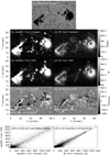 |
Fig. 6. Same as Fig. 5, but for SHARP No. 4375. |
| In the text | |
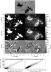 |
Fig. 7. Same as Fig. 5, but for SHARP No. 5118. |
| In the text | |
Current usage metrics show cumulative count of Article Views (full-text article views including HTML views, PDF and ePub downloads, according to the available data) and Abstracts Views on Vision4Press platform.
Data correspond to usage on the plateform after 2015. The current usage metrics is available 48-96 hours after online publication and is updated daily on week days.
Initial download of the metrics may take a while.