| Issue |
A&A
Volume 647, March 2021
|
|
|---|---|---|
| Article Number | A168 | |
| Number of page(s) | 14 | |
| Section | Stellar structure and evolution | |
| DOI | https://doi.org/10.1051/0004-6361/202039578 | |
| Published online | 29 March 2021 | |
Searching for solar-like oscillations in pre-main sequence stars using APOLLO⋆
Can we find the young Sun?
1
Institut für Astro- und Teilchenphysik, Universität Innsbruck, Technikerstraße 25, 6020 Innsbruck, Austria
e-mail: marco.muellner@student.uibk.ac.at
2
INAF – Osservatorio Astrofisico di Catania, Via S. Sofia 78, 95123 Catania, Italy
3
Institute of Solar-Terrestrial Physics, Siberian Branch of Russian Academy of Sciences, Lermontov Str. 126A, 664033 Irkutsk, Russia
4
Thüringer Landessternwarte Tautenburg, Sternwarte 5, 07778 Tautenburg, Germany
5
South African Astronomical Observatory, PO Box 9, 7935 Observatory, Cape Town, South Africa
6
Southern African Large Telescope Foundation, PO Box 9, 7935 Observatory, Cape Town, South Africa
7
Sternberg Astronomical Institute, Lomonosov Moscow State University, Moscow 119234, Russia
8
Space Research Institute, Russian Academy of Sciences, Profsoyuznaya 84/32, 117997 Moscow, Russia
Received:
2
October
2020
Accepted:
14
December
2020
Context. In recent years, our understanding of solar-like oscillations from main sequence to red giant stars has improved dramatically thanks to pristine data collected from space telescopes. One of the remaining open questions focuses on the observational identification of solar-like oscillations in pre-main sequence stars.
Aims. We aim to develop an improved method to search for solar-like oscillations in pre-main sequence stars and apply it to data collected by the Kepler K2 mission.
Methods. Our software APOLLO includes a novel way to detect low signal-to-noise ratio solar-like oscillations in the presence of a high background level.
Results. By calibrating our method using known solar-like oscillators from the main Kepler mission, we apply it to T Tauri stars observed by Kepler K2 and identify several candidate pre-main sequence solar-like oscillators.
Conclusions. We find that our method is robust even when applied to time-series of observational lengths as short as those obtained with the TESS satellite in one sector. We identify EPIC 205375290 as a possible candidate for solar-like oscillations in a pre-main sequence star with νmax ≃ 242 μHz. We also derive its fundamental parameters to be Teff = 3670 ± 180 K, log g = 3.85 ± 0.3, v sin i = 8 ± 1 km s−1, and about solar metallicity from a high-resolution spectrum obtained from the Keck archive.
Key words: asteroseismology / methods: data analysis / stars: interiors / stars: pre-main sequence / stars: solar-type / stars: individual: EPIC 205375290
© ESO 2021
1. Introduction
Asteroseismology is the most powerful method to describe the inner structure of stars. In recent years, several space missions have delivered pristine photometric data that have significantly advanced our knowledge of stellar interiors and the physical processes acting inside stars.
Two of the pioneering space telescopes for asteroseismology were the Canadian microsatellite MOST (Microvariability and Oscillations of Stars; Walker et al. 2003) and the french-led mission CoRoT (Convection, Rotation, and Planetary Transits; Auvergne et al. 2009). These were followed by the NASA Kepler (Borucki et al. 2010; Koch et al. 2010) space telescope. After the failure of two reaction wheels aboard Kepler in 2013, the mission continued as K2 (Howell et al. 2014) with a different observing strategy.
Solar-like oscillations are caused by turbulent convective motions near the stellar surface and show p-modes in its frequency spectrum (Chaplin & Miglio 2013; García & Ballot 2019). These types of oscillations have very small amplitudes, making space missions the primary driver for detecting them. The previously mentioned space missions, starting with CoRoT (e.g., Michel et al. 2008; De Ridder et al. 2009), were especially impactful in the search for solar-like oscillators.
The greatest progress by far has been made by studying solar-like oscillations in main sequence (MS) and red giant stars (e.g., Lund et al. 2017; Bastien et al. 2013; Huber et al. 2011; Antoci et al. 2011). These p-mode pulsations are driven by the outer convective layer, have pressure as their restoring force, and are described by two typical parameters: the large frequency separation (Δν) and the frequency of maximum power (νmax). Scaling relations connect these two asteroseismic observables with the stellar fundamental parameters (Kjeldsen & Bedding 1995; Huber et al. 2011) and are based on the observed values for the Sun.
All of the present observational studies of solar-like oscillations describe stars starting from the main sequence phase of stellar evolution. For a complete evolutionary picture, it is essential to connect the early phases of stellar evolution with the later phases is essential. We aim to understand the properties of ‘young Suns’ in terms of activity and rotation (e.g., Fröhlich et al. 2012) to be able to trace the Sun back to its initial conditions. In this, the next logical step is to investigate the oscillatory past of the Sun and solar-like stars by searching for solar-like oscillations in pre-main sequence (pre-MS) stars.
The presence of solar-like oscillations in pre-MS stars was proposed by Samadi et al. (2005) and Pinheiro (2008) based only on theoretical calculations. Until today no pre-MS solar-like oscillators have been detected observationally. This is due to the high degree of activity present in young stellar objects, which introduces a high background and obscures any oscillation signal, but is also caused by suppression of oscillation mode amplitudes due to the presence of magnetic activity (Chaplin et al. 2011; Bonanno et al. 2014), which further reduces the signal to noise ratio (S/N), making detections very difficult. Consequently, one important aspect of our search for pre-MS solar-like oscillators is the formulation of the background. Progress in terms of background formulation was discussed by for example Mathur et al. (2011a), Karoff (2012), Kallinger et al. (2014, 2016), and Corsaro et al. (2017).
Another reason for the small number of observational discoveries of PMS solar-like pulsators so far is the lack of high-precision photometric time-series of young stellar objects preferably from space and with sufficiently long time bases. As the main Kepler mission was purposefully pointing away from young star-forming regions, the current maximum observing lengths for pre-MS pulsators is on the order of 80 days from Kepler K2 (Howell et al. 2014) and up to about 105 days as obtained using data collected by the NASA mission TESS (Ricker et al. 2014). Also, these relatively short observational time bases impact the noise sources that therefore have to be treated properly when searching for low-amplitude stochastic oscillations.
T Tauri stars are the main candidate pre-MS objects to search for solar-like oscillations. These young stars, which are usually of spectral types late F, G, K, and M, have recently become visible in the optical and have masses ≲2 M⊙. Their light variability can vary over a large range of timescales, from minutes to decades, and show both regular and irregular behaviour (e.g., Alencar et al. 2010; Cody et al. 2014). Furthermore, the size and location of their outer convective regions resemble those of solar-like stars.
Space missions such as Kepler, TESS, and the future ESA mission PLATO (Rauer et al. 2014, expected launch in 2026) have already brought asteroseismology into the era of big data: With sample sizes on the order of a minimum of half a million objects, new methods and pipelines are required for the analysis of stellar oscillations that allow for automated processing. These methods are required to be computationally efficient, to process large datasets in a reasonable amount of time, and to yield reliable results, which is made possible by rigorous statistical methods such as the Bayesian approach used in the present work. Previous works from Campante et al. (2016) and Schofield et al. (2019) discussed the detectability of solar-like oscillations from TESS observations, both from a theoretical standpoint and from the nominal photometric performance of TESS.
In this work, we present the APOLLO (Automated Pipeline for sOlar-Like Oscillators, available online1) pipeline. In addition to computing the background, APOLLO includes a novel way to detect low S/N solar-like oscillators by applying model comparisons in a ‘blind’ way. For this, a Bayesian approach based on DIAMONDS (Corsaro & De Ridder 2014) is used, which allows the user to quantify the significance of a signal in a given dataset. We apply APOLLO to known solar-like oscillators and calibrate the method. In a final step, we investigate data from the K2 mission for potential pre-MS solar-like oscillators with APOLLO and present the first candidates.
2. Target selection
2.1. Main sequence and post-main sequence star sample
For the development and calibration of our method, we selected 1119 solar-like oscillators observed by the Kepler satellite, provided through the KASC2 collaboration (Kjeldsen et al. 2010). Of these 1119 objects, 1071 are obtained in long cadence (LC; sampling time Δt = 29.45 min; Jenkins et al. 2010), representing a sample of evolved red-giant stars with available fundamental properties from photometry, as well as spectroscopic parameters from the APOKASC catalogue (Pinsonneault et al. 2014); 48 targets are short cadence (SC; sampling time Δt = 59.89 s Gilliland et al. 2010), giving us our subset of main sequence and subgiant stars from the LEGACY sample (Lund et al. 2017), for which fundamental asteroseismic parameters are available from the literature.
All the red giants in our sample have been observed for at least two years, with 60% having four years of nearly continuous measurements. We did not explicitly impose limiting values of effective temperature and magnitude on any of the stars during our selection, apart from the constraints of the APOKASC catalogue. Accordingly, the frequency spectra of the selected red giants cover νmax values ranging from 1 μHz to 246 μHz.
The SC sample consists of both ‘Simple’ and ‘F-Type’ stars, following Appourchaux et al. (2012). These stars have an observation baseline of at least 370 d, with 59% showing a baseline of 1095 d (∼3 yr). The frequency ranges for these stars cover νmax values between 885 μHz and 3456 μHz, representing our main sequence and subgiant sample. Additionally, effective temperatures and Kepler magnitudes, Kp, for our full sample of 1119 stars were extracted from the Kepler input catalogue (Brown et al. 2011) to estimate νmax.
2.2. Candidate pre-main sequence solar-like stars
For our search for pre-MS solar-like oscillators, we identified 135 candidate pre-MS solar-like oscillators in the data from the K2 mission Campaign 2, which partially observed the Upper Scorpius (USco) subgroup. This group is one of three that belong to the Scorpius-Centaurus OB Association (Sco-Cen) and also the youngest one with 10 ± 3 Myr. The 135 selected stars all show an effective temperature of between 4500 and 7000 K, are members of USco, and consequently are identified as pre-MS stars. To obtain the surface gravity, log g, effective temperature, Teff, and radii of these stars used for the identification process of solar-like oscillation, we use the Ecliptic Plane Input Catalog (EPIC) by Huber et al. (2016).
3. Methodology
The methodology used in the APOLLO pipeline is designed to determine the asteroseismic parameters νmax and Δν of solar-like oscillators by exploiting a Bayesian approach. For this, we only consider the light curve, effective temperature and magnitude of a given star. The following subsections describe our method in detail.
3.1. Data preparation
The light curves used in this work were provided by KASC and directly downloaded from their website, which already includes the reduction using the KASOC filter (Handberg & Lund 2014).
As our first step, we create a histogram of the relative flux values which is then fitted with a normal distribution, providing its mean and standard deviation, σ. All data points outside 4σ are then removed from the light curve and gaps longer than three days are linearly interpolated connecting the two points adjacent to the gap.
For these resulting light curves we compute the power spectral density (PSD) using the Lomb-Scargle periodogramm (Lomb 1976; Scargle 1982) normalised using Parseval’s theorem and finally converted to the PSD by dividing through the integral of the spectral window. This PSD is the main input for our further analysis.
3.2. Bayes theorem and model comparison
The core of our analysis is based on the Bayes theorem, which is formulated as
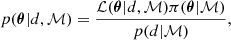
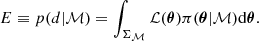
where θ is the parameter vector consisting of the free parameters of the model ℳ applied to the data set d, which is in our case the stellar PSD. The likelihood function ℒ(θ|d, ℳ) represents the way the data are sampled. To describe Fourier power spectra, (i.e. our PSD), it is necessary to adopt the exponential likelihood as introduced by Duvall et al. (1986) and Anderson et al. (1990). The parameter π(θ|ℳ) denotes the prior probability density function (PDF) defined through their respective prior distributions. The denominator in Eq. (1) is the Bayesian evidence (also called marginal likelihood or model performance), giving us a quantitative evaluation of the quality of the model in light of the data. It is defined by
This value is of critical importance for the model comparison. Assuming two distinct models ℳi and ℳj, we can apply these two models to our data set d. We can then take their respective evidence Ei and Ej, and compute the odds ratio Oij, defined by
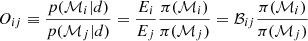
comparing the evidence for both models. For our purpose, we set both model priors π(ℳ) = 1/2, as we give both models equal probability for a given data set, and therefore the odds ratio is equal to the Bayes factor with Oij = ℬij. Using the empirical scale of strength shown in Table 1, we can then determine the favoured model.
Empirical scale for comparison of the strength of evidence to determine the Bayes factor (Trotta 2006).
3.3. The models
As described in Sect. 3.2, we need two distinct models that are applied to the PSD. For this we use two variants of the background model based on those presented by Mathur et al. (2011b), Karoff et al. (2013), and Kallinger et al. (2014). We call these two models the oscillation model Posc(ν) and noise model Pnoise(ν).
The oscillation model Posc(ν) can be expressed as
![$$ \begin{aligned} P_{\rm osc}(\nu )=\sigma _{\rm b}+R(\nu )[B(\nu )+G(\nu )] \end{aligned} $$](/articles/aa/full_html/2021/03/aa39578-20/aa39578-20-eq4.gif)
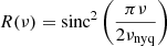
where σb is assumed to be a flat noise level and R(ν) the response function, which takes the sampling rate of observations into account, defined by
with νnyq being the Nyquist frequency from either the LC or SC observation modality, defined by half of the sampling rate of the signal. The components related to the granulation activity and long-term trend of the star, B(ν), are expressed as a series of Harvey-like functions, given by
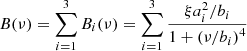
which are defined by the root mean square (rms) amplitude of the components ai and the characteristic frequency bi, where bi is the frequency at which the power of the component is half than that at zero frequency. The factor ξ is used to normalise ![$ \int_{0}^{\infty} (\xi/b)/\left[ 1 + (\mathit{v}/b)^{4} \right] \mathrm{d}\mathit{v} = 1 $](/articles/aa/full_html/2021/03/aa39578-20/aa39578-20-eq7.gif) , such that the measured ai actually corresponds to the rms amplitude measured in the light curves, hence yielding
, such that the measured ai actually corresponds to the rms amplitude measured in the light curves, hence yielding  .
.
The oscillation region of a solar-like oscillator is characterised by a power excess. Here, we describe the power excess, G(ν), by a Gaussian function:
![$$ \begin{aligned} G (\nu ) = H_{\rm osc} \exp \left[- \frac{\left(\nu - \nu _{\max }\right)^{2}}{2\sigma _{\rm env}^{2}}\right] \end{aligned} $$](/articles/aa/full_html/2021/03/aa39578-20/aa39578-20-eq9.gif)
where Hosc, νmax, and σenv are the height, central frequency and standard deviation of the Gaussian corresponding to the power excess.
The second model in this work, Pnoise(ν), is a variant of the oscillation model Posc(ν). In this model we remove the power excess, leaving us with the equation

giving us ten free parameters for Posc(ν) and seven for Pnoise(ν). We note that many components of our models often exhibit strong correlations that may arise among several of their free parameters. For this reason, we choose to apply a Bayesian approach based on the nested sampling algorithm (Skilling 2006), which is suited for finding solutions for parameter-degenerate cases.
The next step is to determine priors for the free parameters of each background model using the PSD of a given object and then feed these priors into DIAMONDS, a Bayesian Nested sampling code, which will then allow us to determine both the parameter estimates of a given model as well as the corresponding Bayesian evidence. The Bayesian evidence will therefore be used to perform model comparisons. The following two sections provide the details on the determination of the priors for DIAMONDS.
3.4. Determination of priors
An inherent part of every Bayesian approach is the selection of good priors for the analysis, and considerable care should be applied. In this section we describe the process of finding priors for the model Posc. This is done by computing estimates of all ten free parameters, and by creating prior distributions from those estimates.
3.4.1. Estimation of νmax
The most important free parameter in the model Posc described in Sect. 3.3 is the frequency of maximum oscillation power, νmax. This is a characteristic value of a given solar-like oscillator, from which most of the other free parameters can be directly inferred using relatively simple relations (e.g., Stello et al. 2008; Kallinger et al. 2010, 2014; Pande et al. 2018) which can in turn be used to set up their prior distributions.
The estimation algorithm for νmax used in the APOLLO pipeline needs to fulfill the following criteria:
-
It must be computationally inexpensive both for SC and LC data.
-
It must provide reasonable accuracy, in the sense that the model-fitting process described in Sect. 3.5 is able to find the correct value for νmax.
-
It needs to work for all evolutionary stages of solar-like oscillators.
-
It must be able to estimate νmax even if the power excess is not clearly distinguishable.
There are multiple approaches to estimate νmax for a given star. Most of them rely on the correlation between the granulation properties of the star and νmax. For example Bastien et al. (2013), using their Flicker method, showed that it is possible to infer νmax from the variation of the stellar flux in the light curve. However, this method is limited to objects between 2.5 < log g < 4.6 dex, restricting the range of stars that can be analysed with our approach.
The method was further improved by Kallinger et al. (2016) who used an iterative approach based on an auto-correlation of the signal. We originally adopted this method for obtaining a good estimate of νmax. Nevertheless, we find that it comes with some drawbacks, especially for SC observations with a long baseline. This is because the auto-correlation of a light curve with on the order of 105 data bins, as in the case of Kepler SC data covering 3−4 years of observation, is computationally expensive, and therefore significantly slows down our pipeline.
Another potential method for estimating νmax is that presented by Bell et al. (2019), who estimate νmax using the coefficients of variation. Their method mimics the process of visually inspecting a PSD and locating νmax, by finding local excesses in power. However, this process only works where the power excess is distinguishable from the background and is the reason why this method is not ideal for our approach, as our method should also be applicable to noisy data, where the power excess cannot be clearly distinguished from the noise.
Finally, Bugnet et al. (2018) proposed the FliPer method, which is analogous to the Flicker method but applied directly to the PSD of the star. This method is computationally inexpensive, it provides reasonable values for νmax even with low S/N data, and it works in all evolutionary stages of solar-like oscillators. We therefore choose to adopt it for this work. An exhaustive description of the method can be found in Bugnet et al. (2018). In summary, the FliPer metric links the variability from all timescales to the surface gravity, log (g), which in turn is linked to νmax. This metric is given by
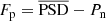
where  is the mean of the power spectral density and Pn is the photon noise. Fp is determined by a combination of granulation and oscillation power, both heavily dependent on the evolutionary stage of the star, as well as on its rotation.
The computation of the FliPer metric is only applied to LC data. If the pipeline is applied to a SC light curve, it will automatically rebin this light curve to fit into a LC light curve, which is then used to compute the FliPer. Further, the computation of the photon noise in the original work by Bugnet et al. (2018) was done using Kp and the empirical relation in Jenkins et al. (2010). In this work we make use of the adapted method from Bugnet et al. (2019) to compute this background noise Pn. This is done by averaging the last 100 data points adjacent to the Nyquist frequency. While the original method from Bugnet et al. (2018) yields a value for νmax closer to the literature values from the APOKASC catalogue, this approach is also useful if there is no Kepler magnitude available for a given star.
The resulting values for νmax, FliPer are shown in Fig. 1. The FliPer metric provides us with reasonable values of νmax, thus allowing us to adequately set up priors for the remaining free parameters of the background models. For incorporating cases where the estimated νmax may not be very accurate, we consider an adequate search range for the fit, as the blue shaded regions indicate. These regions (representing the 1-σ range where we expect νmax using FliPer, given the standard deviation of our prior for νmax) all include the corresponding values from the APOKASC catalogue.
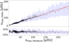 |
Fig. 1. Upper panel: values for νmax extracted from the FliPer method as compared to the values from the APOKASC catalogue. Lower panel: corresponding residuals as percentile. The red shaded area represents the uncertainties in the catalogue. The blue shaded areas define our 1-σ interval, centred around νmax from FliPer. |
However, in general the FliPer values alone already give us a good estimate of νmax, as shown in the distribution of Fig. 2. This distribution shows that the FliPer value for νmax exhibits a systematic deviation of 4.95% and a random error within 1-σ of 6.93% with respect to the values reported in the literature.
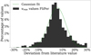 |
Fig. 2. Distribution of values for νmax extracted from the FliPer method. The Y axis shows the percentage of values within a given bin of deviation from a corresponding literature value, while the X axis shows the deviation from the literature value in percent. The distribution can be represented by a Gaussian function, whose fit to the histogram is represented by a dotted green line. The mean for this distribution is at 4.95%, with a standard deviation of 6.93%. For visualisation purposes, deviations above 30% and below −30% are excluded. |
3.4.2. Determination of priors for the full background model
The parameters a2, a3, b2, and b3, which define two of our three Harvey-like functions in Eq. (6), are estimated using scaling relations from Kallinger et al. (2014), which relate these parameters directly to νmax. For our first Harvey-like function, representing the long trend variation, we adapt the following: a1 is estimated using the same scaling relations as a2 and a3, and the prior distribution for b1 is directly determined and not calculated (see Tables 2 and 3). The flat background noise, σb, is determined by computing the median of the adjacent 100 points to the Nyquist frequency, and converting it to the mean using the relation between median and mean for the χ2 distribution with two degrees of freedom (Appourchaux 2014). These seven parameters (a1, a2, a3, b1, b2, b3, and σb) fully estimate Pnoise(ν) and are also used for the Harvey-like function and background noise in Posc(ν). The remaining free parameters for which an initial guess has to be obtained are Hosc and σenv, which are related to the Gaussian envelope presented in Eq. (7). The parameter Γenv, namely the full width at half maximum of the Gaussian envelope, is determined using (Mosser et al. 2012)
Prior ranges for our red-giant sample.
and it is related to σenv with
An estimation for Hosc can instead be found using νmax and σenv to restrict the PSD to the region νmax − σenv < ν < νmax + σenv, hence computing the median in this region to get our estimate of Hosc. This concludes our set of ten parameters for Posc(ν).
We have in principle multiple options to use these input guesses for the free parameters of the models when constructing priors because it is possible to adopt different prior distributions in a Bayesian inference process. Generally we choose to use flat (i.e. uniform) priors for all parameters except νmax. Even if we have an estimate for a central value for each of the free parameters as described above, we still prefer to adopt uniform priors for most of them because some of the parameters exhibit an interval of variation that could be well constrained from scaling relations, and because uniform priors are computationally the most efficient ones. For νmax instead, it is more critical to make sure that the actual value of this parameter is properly fitted during the Bayesian inference. This is because our aim is to detect the presence of a possible power excess in an automated way, meaning that identifying the correct location of the power excess is a mandatory step to make the whole analysis successful. The prior knowledge through our analysis of the FliPer metrics, which takes into account the systematic and random errors in the FliPer as seen in Fig. 2, suggests that a normal distribution represents an adequate choice for the prior of this parameter. This confers the additional advantage that we further mitigate fluctuations in our estimation of νmax. This is because normally distributed priors are not as restrictive as flat priors, meaning that there is a non-zero prior value along the full range of the given free parameter. Flat priors in contrast, assign an equal prior probability within a given range and a sharp transition to zero prior probability outside of the prior range, thus cutting out any possibility of detecting the actual value of the free parameter in case this is falling outside the prior boundaries.
3.5. Background fitting and DIAMONDS
To fit the models Posc and Pnoise to a given PSD, we apply the Bayesian parameter estimation tool DIAMONDS3 (Corsaro & De Ridder 2015). DIAMONDS applies Bayes theorem, as described in Sect. 3.2. Equation (2) is a multi-dimensional integral and as the number of dimensions increases, solving it becomes very hard both analytically and numerically. DIAMONDS overcomes this problem by applying the Nested sampling Monte Carlo (NSMC; Skilling 2006) algorithm. This algorithm samples both the posterior probability distribution and the Bayesian evidence, which in the context of this work is used to compare the models Posc and Pnoise and simplifies the multi-dimensional problem of Eq. (2) to a one-dimensional problem. The simplification is done by considering the prior mass dX = π(θ|ℳ)dθ such that
defining a fraction of volume under the prior PDF constrained by ℒ*, with ℒ* being some fixed value of the likelihood. This therefore reduces to a one-dimensional integral with
Assuming that one has Nnest pairs of  , Eq. (13) can be rewritten as
In practice, this is solved by iteratively setting a likelihood constraint that is higher than a previous one for each iteration, peeling off a thin shell of prior mass and evaluating the evidence using Eq. (14). Nevertheless, the NSMC algorithm can quickly become computationally expensive because of the increasing difficulty in obtaining new good sampling points at each iteration. DIAMONDS overcomes this problem by applying simultaneous ellipsoidal sampling (SES; Feroz & Hobson 2008; Shaw et al. 2007) based on a preliminary clustering of the set of live points at a given iteration.
DIAMONDS also allows different prior distributions to be chosen for different parameters of our models. This is specifically useful for our approach and not a standard feature in other existing codes of this kind. The parameter ranges for all free parameters are given in Table 2 for LC data and Table 3 for SC data. These should be interpreted as variations around the central values determined in Sect. 3.4.2 and are made small enough to allow DIAMONDS to efficiently converge to a solution, but are also large enough to properly account for uncertainties in the free parameters. For the amplitudes ai and Hosc a large range was given deliberately due to the character of the fitting process and due to the large variations in the parameter value and dependencies on other parameters. A special case is the prior b1, the cutoff frequency of the first Harvey component. The parameter b1 is not directly inferred from the PSD or from νmax. For b1 to be appropriate, it always has to fulfill νmin < b1 < min(b2), where νmin equals the smallest frequency in the power spectrum and min(b2) the lower end of the prior for b2.
The priors described in the previous sections are used by DIAMONDS to fit both models Posc and Pnoise to the power spectral density of a given star. The estimated parameters, including their marginal distributions, as well as the Bayesian evidences Eosc and Enoise, for models Posc and Pnoise respectively, are all outputs of the fitting process. Using their respective evidence, we compute the odds ratio of the models Oosc, noise and using the empirical scale of strength shown in Table 1 we determine if the oscillation model Posc is to be favoured over the noise model Pnoise, giving us an indication of whether or not there is an oscillation signal for a given data set.
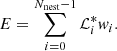
This is especially useful for power spectra where a power excess is not clearly distinguishable by eye. One example, that shows the potential of this approach is illustrated in Fig. 3. In this example the method is applied to a test star from our sample of red giants, using an observation length of 1400 days, 109.6 days, and 27.4 days. It appears that in the case of 27.4 days, we can no longer clearly discern the oscillation region anymore in the PSD. If the atmospheric properties of the star, such as surface gravity and effective temperature, are available, it is possible to predict the frequency position of a power excess in the region where it is actually found. In real applications with similar S/N as in the example shown in Fig. 3, visual inspection alone is insufficient to claim a detection.
 |
Fig. 3. fIT provided by DIAMONDS for three different observation lengths for KIC 9903915. Upper row: full background model, lower row: noise only model. Different observation lengths are split into three columns: first column: result for the full 1400 day light curve, second: for 109.6 days and third: for 27.4 days. We find strong evidence for all three observation lengths: log O = 990.53 for 1400 days, and log O = 75.42 and log O = 13.86 for 27 days. Even at 27 days we are still above the threshold of log O = 5 for strong evidence. |
3.6. Determination of Δν
The pipeline also determines the large frequency separation Δν if the fit of the background model is successfully applied. For this, we no longer rely on a Bayesian approach, but use classical means. We subtract the background without the Gaussian envelope from the PSD of the star and restrict the resulting spectrum to the oscillation region through the determined values for νmax and σenv. This region is first slightly smoothed and then auto-correlated, allowing us to detect the typical regularity in the frequency pattern of the p modes. Through the well-known relation between νmax and Δν (Stello et al. 2009) we can compute an initial guess for Δν using
by Huber et al. (2011). Using this value as a reference, we can locate the closest peak that is obtained from the auto-correlation. We then fit a normal distribution to this peak and take its resulting mean as the estimated Δν.
4. Implementation of the APOLLO pipeline
APOLLO is a fully integrated Bayesian fitting pipeline. Its core is written in Python, with extensive use of highly optimised scientific libraries (Virtanen et al. 2020; Oliphant 2006; Astropy Collaboration 2013, 2018). It also makes direct use of DIAMONDS, for which we created both a Python interface as well as direct parsing of the binary output. The pipeline also generates the necessary run files for DIAMONDS and analyses its outputs. It possesses full multi-processing capabilities, allowing the analysis of multiple stars in parallel when modern multi-core processors are in use. This allows for quick evaluations of large data sets: Our sample of red giants, consisting of 1071 objects with the majority having four years of observation and consisting of around 68 000 data points, takes six hours to complete using the AMD Threadripper architecture with all 32 threads in use. Extrapolating from this, the average run time for one object, including the fit for both models, takes around 20 s. In comparison, performing the analysis sequentially (one star at a time on one thread) takes between five and ten minutes per star.
The pipeline is also highly configurable. It uses the JSON format as input and output files, which allows machine readability as well as the possibility for humans to read these files and interpret their content. The input files contain various configuration flags, making the pipeline very flexible for various uses. The output files contain all results from DIAMONDS, as well as priors, estimations of parameters and a myriad of other data, that can be used to further analyse the result.
The full code as well as documentation and examples are available at the github repository4. All further improvements and changes will also be available there.
5. Calibration
5.1. Reliability of the method
The first step in the analysis using APOLLO is to compare the results obtained with the pipeline to the results from the APOKASC and LEGACY samples, both consisting of stars observed with Kepler, which we use in this work to check the robustness of the method. We also introduce the term completion rate, which is the number of completed runs for a given sample of stars. In order for a run to qualify as completed, the following four criteria must be fulfilled:
-
The estimations of the free parameters must have been successfully carried out by DIAMONDS, meaning that the code was able to perform a fit for both background models without errors.
-
The Bayes factor Oosc, noise as defined in Eq. (3) must exceed the criterion of strong significance, which is Oosc, noise > 5.
-
Runs that result in a νmax outside of 1σ of the values from APOKASC and Legacy catalogs are manually checked and discarded if their fit is not correct. If this is not the case, the results are kept, even if νmax is outside of 1σ of the catalogue values. This step is only necessary for the calibration of the method.
-
Power spectra that show contamination by binaries (Colman et al. 2017) are also discarded, if the pipeline does not detect the oscillation region correctly, but rather the excess due to contamination.
Following these criteria, we get a completion rate of 95.5% for our red giant sample, completing 1023 out of 1071 objects. The reasons for discarding 48 objects out of the 1071 analysed are twofold:
-
An incorrect estimate of νmax from the FliPer metric is seen for 36 objects. This prevents DIAMONDS from adequately sampling the actual νmax values as the normal prior centroid is far from the proper solution.
-
Twelve objects contain contamination of binaries, which leads to DIAMONDS detecting the excess of the contamination as the oscillation region.
The resulting values from our red-giant sample for νmax for the completed 1023 objects are shown in Fig. 4 and their corresponding values for Δν are shown in Fig. 5. Of these 1023 objects, 65% agree within 1-σ with the catalogue values of νmax. For Δν we find excellent agreement with the literature values, with 91% of all values falling within 1-σ uncertainty from the literature values.
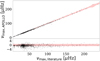 |
Fig. 4. Resulting νmax, APOLLO values of the APOLLO pipeline in relation to catalogue values of our red-giant sample. Upper panel: comparison of νmax, APOLLO to the literature, with the red shaded area illustrating the 1-σ uncertainties in the literature. Lower plot: residuals in sigma of the literature value and again mark the uncertainties in the red shaded area. |
We performed the same analysis for our MS sample. Initially we applied the same boundaries for our priors for both the MS sample and the red giants. The prior distributions for νmax and σenv were consequently too large for the main sequence sample, making it impossible to reliably fit this sample. We therefore restricted the prior distributions further than we did for the red giants. Our estimation of the background noise σb turned out to be too small for some of the MS sample, which we mitigated by slightly increasing the upper limit of the prior distribution for σb.
The resulting values for νmax are shown in Fig. 6. For our dwarfs we find a completion rate of 85%. From the nine objects that failed, no fit was found for three of them, and one object showed a value for ln(Oosc, noise) < 5. The remaining five failed because of an incorrect estimate of νmax from FliPer. For our main sequence sample 35% agree within 1-σ with the values from the LEGACY catalogue. In more detail, 85% agree within 10%, 68% within 5%, and 51% within 3% of the literature value. These large deviations in terms of σ are most likely due to application of a different background model applied by Lund et al. (2017), where they only used two Harvey-like functions, as well as a different representation of the oscillation region through a series of Lorentzian functions.
5.2. Reduction of observation length
With the advent of the TESS space mission, we are now dealing with data sets that exhibit various observing lengths. In this regard, it is also relevant for us to test the performance of the pipeline in observing conditions different from those of Kepler. To do this, we reduce the baseline of the Kepler observations to adapt to those covered by TESS, namely 356.2 d, 109.6 d, 82.2 d, 54.8 d, and 27.4 d. We use the full sample of our red giants, and compute fits for all 1023 objects that were completed using the default baseline, in all of the five observation lengths provided by TESS. The completion rate (from the 1023 objects) yields 100% for Tobs = 356.2 d and 99% for observation times 109.6 d, 82.2 d, and 54.8 d. For our lowest observation time of 27.4 d we find a completion rate of 95%, showing that our pipeline is highly insensitive to the observation baseline, making it very suitable for TESS data.
Again, we compare the results from these fits to the values for νmax from the APOKASC catalogue. The result for our baseline and the five TESS observation lengths is shown in Fig. 7 (left panel). The result shows, as expected, a broadening of the distribution for smaller observation lengths. With the lowest observation time of 27.4 d, 45% of the values for νmax still agree with the literature values within 1-σ. We also find a systematic deviation to the literature values, which can be explained through the choice of a different background formalism.
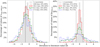 |
Fig. 7. Distribution of values for νmax (left panel) and Δν (right panel) in different observation lengths. Grey filled bars represent the values for 1400 days of observation, and smaller observation lengths are shown in different colours. The red dashed lines represent the 1-σ range of the literature values. The legend states the percentage value of stars within 1-σ. In brackets we note the percentage value when taking the uncertainties of the fit into account. For νmax, using 27 d observations 19.88% of our sample falls outside of the 1-σ range in comparison to the full observation length. For Δν this decrease is much stronger, with 83.91% of the sample falling outside of 1-σ using 27 d of observation. |
By comparing the result for Δν from the pipeline to the catalogue values, the effect of shorter observation lengths is significantly stronger than that of νmax. As can be seen by looking at Fig. 7 (right panel), we find a strong broadening of the distribution, especially for the very short observing lengths. This is an effect of the reduced S/N in stars with short observation lengths and is amplified by the decreasing resolution of the power spectrum. This is reflected in the total values falling within 1-σ of the catalogue values: For 109.6 d already, only 50% of all objects fall inside the uncertainty. Using 27.4 d reduces this further to only 7%.
5.3. Detection of fainter stars
To simulate the expected magnitude range of stars extracted by the TASC photometry pipeline (Handberg & Lund 2019) for the red-giant sample, we add random, normally distributed noise to the light curves of a sample of stars. We compute the white noise from the PSD by calculating the mean of the preceding 100 data points below the Nyquist frequency. In the following we convert this noise to the corresponding Kepler magnitude Kp and relate this to the TESS magnitude IC with IC = Kp − 5 (Stassun et al. 2018) using the relation by Pande et al. (2018).
The actual sample used for this simulation test is obtained by reducing our initial sample of Kepler red giants based on the following conditions:
-
We restrict ourselves to stars that follow the relation from Pande et al. (2018) within 0.4 mag, to reduce the uncertainty in the calculated magnitudes from the white noise.
-
We choose stars that show a magnitude in the range of 11.6 mag < Kp < 12 mag. This allows us to simulate sufficient points to the faintest objects at 15 mag (IC = 10 mag) and assigns all simulated stars a similar starting value.
-
All objects must fall within 1-σ of the catalogue values for νmax
Applying these criteria yields 84 valid objects which are shown in Fig. 8. From this sample we compute ten snapshots of white noise level, corresponding to magnitudes within 12 mag < Kp < 15 mag, a range that incorporates the upper limit considered in the TASC data preparation. For a given magnitude, we run our method for all sample stars three times, and average the resulting three values for the Bayes factor of each star in order to mitigate statistical deviations. The resulting averaged Bayes factor values for each star and magnitude are again averaged, giving us the central value  and uncertainty for a given magnitude. Using this value, we can then estimate up to which magnitude the oscillations are still detectable.
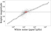 |
Fig. 8. Relation between Kepler magnitude Kp, and white noise. The black solid line represents the relation from Pande et al. (2018), the grey shaded area represents the white noise range corresponding to a variation of 0.4 mag. Our sample is represented by the grey and red dots, where the red dots constitute the sample used in the magnitude analysis, and is identified by the intersection of the horizontal lines with the grey shaded area. The horizontal grey dashed lines show the range of these points within 11.6 mag < Kp < 12 mag. |
The result is illustrated in Fig. 9. As expected, we find a decrease in  proportional to the observation length of the data sets. The Bayes factor is highest for bright objects with long observation baselines, which is a natural result of having a better S/N and a higher frequency resolution in the PSD of the star than for fainter magnitudes and shorter observing lengths. Longer observation times give us a stronger shape of the power excess and an equal increase in the significance of the full background model. Despite this, Oosc, noise still exceeds the significance threshold of ln(Oosc, noise) = 5 for all observation lengths and magnitudes up to Kp = 15 mag (IC = 10 mag), making it possible, in principle to detect solar-like oscillations in faint red giants up to Kp = 15 mag (IC = 10 mag) even with an observation length of 27.4 d.
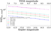 |
Fig. 9. Relation between Bayes factor Oosc, noise and Kepler magnitude as well as the converted TESS magnitude. Different observation lengths are color coded. |
A similar analysis was also done for the main sequence sample, except in this case we used the complete sample. This clearly shows a different picture from that for red giants as illustrated in Fig. 10. The main sequence sample is much more sensitive to the brightness of the object, and already approaching the significance threshold for observation lengths Tobs = 54.8 days for fainter stars. This is due to the fact, that main sequence solar-like oscillators are much fainter, following the luminosity-mass and amplitude relation (Corsaro et al. 2013), show a much lower oscillation amplitude. Therefore, it is intrinsically harder to find solar-like oscillation in main sequence stars than in red giants.
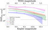 |
Fig. 10. Relation between Bayes factor Oosc, noise and Kepler magnitude for the main sequence sample. |
6. Searching for pre-main sequence solar-like oscillators
6.1. Pre-main sequence models
We use version r-11701 of the software Modules for Experiments in Stellar Astrophyscis, MESA, (Paxton et al. 2011, 2013, 2015, 2018, 2019) to construct a set of non-rotating stellar models with initial masses of between 0.2 and 5.15 M⊙ and initial abundances Z = 0.02 and Y = 0.28. These stellar models are evolved from the Hayashi tracks until the zero-age main sequence (ZAMS). We choose to evolve the models without mass loss or accretion and with an Eddington-Grey atmosphere. The treatment of convection is via the mixing length theory with mixing length αMLT = 1.8 and convective premixing, introduced in Paxton et al. (2019).
Using the scaling relation
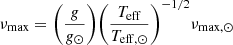
we can estimate νmax for the computed stellar models and compare with the Nyquist frequency of LC data. The Nyquist frequency represents a natural upper limit to the detectable νmax values. We therefore locate the position in the log Teff − log g diagram at which the estimated νmax attains the Nyquist frequency of LC data. The results are shown in Fig. 11, which also shows two versions of the location of the birthline5 according to the description of Palla & Stahler (1990) and Behrend & Maeder (2001).
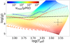 |
Fig. 11. Evolutionary tracks in a log Teff − log g diagram. The colour code describes νmax obtained from the scaling relation. The black line shows the location at which νmax is equal to the Nyquist frequency of LC data. The red and blue lines show the locations of the birthline according to Palla & Stahler (1990) and Behrend & Maeder (2001), respectively. The black crossed object shows the spectroscopic observations for EPIC 205375290. |
The birthline describes the evolutionary track of an accreting protostar. After the star has accreted its final mass, it evolves along the evolutionary tracks shown in Fig. 11. Consequently, it is very unlikely to observe stars that lie above the birthline. Therefore, LC data only allow the detection of solar-like oscillations in pre-MS stars for the small portion of evolutionary tracks that lie below the birthline and above the black dashed line showing the Nyquist frequency in Fig. 11.
6.2. Pre-main sequence solar-like candidates
In a first step we apply the Everest pipeline by Luger et al. (2016, 2017) on our sample of 135 pre-MS stars to remove instrumental noise. The oscillation frequencies of optically visible pre-MS solar-like oscillators are expected to be above 100 μHz (see Fig. 11). Therefore, we can safely filter out the frequencies in the lower frequency ranges that are caused by interactions between the star and its surrounding disc as well as activity in the star. This is also necessary, as the amplitude of these low frequency variations are significantly higher than the expected amplitude of the oscillations. Not removing these variations would make it impossible to detect potential oscillations in our sample. We therefore apply a Savitzky-Golay (Savgol) filter (Savitzky & Golay 1964) and choose a third-order polynomial with a window size between 41 and 331, depending on the individual data set.
In the next step, we use the FliPer method (see Sect. 3.4.1) and the scaling relation from Eq. (16) under the assumption that both relations are valid for pre-MS solar-like oscillations, and estimate the stars’ surface gravity to log gFliPer. We then compare log gFliPer to log gEPIC from the EPIC catalogue for every star. If we can find agreement between log gFliPer and log gEPIC, we mark that star as a potential pre-MS solar-like candidate. This requirement is fullfilled by 13 stars which are listed in Table 4.
APOLLO results for all LC candidates.
As expected, most of the candidates have an expected νmax larger than the Nyquist frequency of 258.4 μHz for LC K2 data. As no SC observations are available for these targets, we restrict our analysis to the narrow region between the Nyquist frequency and the birthline(s) as illustrated in Fig. 11. This leaves us with five objects for further inspection.
We apply APOLLO to each of these five targets five times to reduce statistical fluctuations. The results for the five stars are listed in Table 4. The stars EPIC 204330922, 205152548 and 204222295 are rejected by APOLLO and show a ln(Oosc, noise) < 0, indicating that there is no significant indication of oscillation according to our model comparison approach. This either means that the oscillation signal is not strong enough for us to detect oscillations in these stars, or that these stars do not show solar-like oscillations.
For both EPIC 204447221 and 205375290 APOLLO yields a Bayes factor ln(Oosc, noise) that exceeds the significance threshold ln(Oosc, noise) > 5. To exclude an induced signal through the treatment of the original light curve with the Savgol filter, we increase or decrease the window size by 10 and redo the analysis. In all cases the Bayes factor exceeds the significance threshold. We find disagreement between the final value of log gAPOLLO and log gEPIC, except for EPIC 205375290, which is why we focus on this latter star for further investigation. The resulting fit and light curve for EPIC 205375290 are shown in Fig. 12.
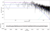 |
Fig. 12. Upper panel: resulting fit for EPIC 205375290. In dashed blue are the Harvey-like functions, the dotted cyan line shows the power excess, the yellow dotted line the white noise, and the red solid line the full fit of the oscillation model. The green line represents a smoothed variant of the PSD. Lower panel: light curve of EPIC 205375290. The filtered and reduced light curve used for the analysis is shown in black while the original light curve is shown in red. |
6.3. EPIC 205375290: a possible candidate
EPIC 205375290 (2MASS J16111534−1757214) is a bona-fide member of the Upper-Scorpius association (RA2000 = 16:11:15.34, Dec2000 = −17:57:21.42) and is listed in SIMBAD as a star of spectral type M1 (Preibisch et al. 2001; Pecaut & Mamajek 2016). The object has a V magnitude of 14.099 (Pecaut & Mamajek 2016) and a J magnitude of 10.227 (Cutri et al. 2003) illustrating a higher flux in the near-infrared.
The APOLLO pipeline yields a νmax of 242(10) μHz and exceeds our significance threshold with ln(Oosc, noise) = 9.07(25). From the scaling relations, we calculate a surface gravity of log g = 3.3(1).
To be able to place EPIC 205375290 in the HR-diagram and learn more about its properties, we first analysed a low resolution (R = 3200) optical spectrum obtained with the RSS spectrograph (Burgh et al. 2003; Kobulnicky et al. 2003) mounted at the South African Large Telescope (SALT; Buckley et al. 2006). We identify Li I 6708 Å to be in absorption and found emission in the hydrogen Balmer lines and Ca II H and K lines. These features are superimposed on a late-type spectrum with prominent TiO absorption bands. Such a spectroscopic pattern is in agreement with the young evolutionary stage of EPIC 205375290. Comparing the depths and shapes of the TiO bandheads with the template spectra from the MILES library (Sánchez-Blázquez et al. 2006), we confirm the spectral class of EPIC 205375290 to be dM1e, which is in agreement with the previous determination by Preibisch et al. (2001).
We then continued our analysis with a high-resolution optical and near-infrared spectrum obtained by the HIRES (High Resolution Echelle Spectrometer) spectrograph at the Keck 1 telescope which is available in the Keck archive6. The observations were taken on June 16, 2006 with the C5 slit which has a width of 1.148″ projected onto the sky resulting in a nominal spectral resolution of R = 38 000. The spectrum covers the range between 4800 and 9200 Å with significant inter-order gaps in the red. It has a S/N of about 35 per pixel (or 80 per resolution element). In addition to the general spectral patterns identified with the low-resolution spectroscopy, the HIRES spectrum revealed the double-peaked profile of Hα emission, a complex structure in the cores of the resonance Na I D lines, emission in the He I line at 5876 Å and emission in the Ca II infrared lines. All these spectroscopic features clearly indicate that EPIC 205375290 is an accreting T Tauri star (Edwards et al. 1994).
The photospheric spectra of T Tauri stars are known to be subject to the veiling effect (e.g., Basri & Batalha 1990; Dodin & Lamzin 2012) which can prevent accurate determination of the atmospheric parameters using the absorption lines. The equivalent width of the Hα emission in EPIC 205375290 is 3 Å and its width at 10% intensity is about 180 km s−1 derived from the HIRES spectrum observed in 2006. According to the criterion from White & Basri (2003), this leads us to conclude that the star is a weak accretor and displays little veiling, if any. However, the slightly redshifted He I 5876 Å emission (i.e. about 5 km s−1 in respect to the stellar rest velocity) indicates the presence of an accretion shock in the system and does not allow us to completely ignore the possible contribution of the non-photospheric continuum or line emission to the observed spectrum of EPIC 205375290. To check this, we fitted the He I 5876 Å line and the accretion-related emission cores in the infrared Ca II triplet (which has the same redshift as the He line) with the pre-computed spectra from the grid of non-local thermodynamic equilibrium (non-LTE) models of accretion shocks in the atmospheres of young stars (Dodin 2015; A. Dodin priv. comm.). The best-fit model which adequately reproduces the observed widths and intensities of accretion-related tracers has an accretion rate of the order 10−11 M⊙ yr−1 and shows no significant veiling of the photospheric lines in the red orders of the HIRES spectrum. Thus, the regions around the infrared Ca II triplet were chosen for further analysis.
We also used a high-resolution (R = 47 000) spectrum of EPIC 205375290 that was obtained with the red arm of the FLAMES-UVES spectrograph mounted at the ESO VLT UT2 telescope. The observations were carried out on 1 June 2016 under programme 097.C-0040(A) and cover the wavelength range from 4800 to 6700 Å with a central gap of ∼150 Å between the detectors. A comparison to the HIRES spectrum revealed the variability of the Hα emission: its equivalent width increased up to 4.1 Å in the FLAMES spectrum. This variability most probably reflects the variations in the accretion rate. A detailed study of the activity of EPIC 205375290 will be the subject of a future work.
For the determination of the star’s fundamental parameters, we used the three HIRES red orders from 8040 to 8120 Å, 8415 to 8555 Å, and 8620 to 8695 Å which contain several atomic lines including the important Ca II infrared triplet at 8498 Å, 8542 Å, and 8662 Å, because this region is almost free from veiling and contamination by the strong molecular bands (see Fig. 13). We avoid using the TiO bands despite their extreme temperature sensitivity because the current state of atomic data for these transitions complicates their use in quantitative analysis (Valenti et al. 1998). We determined the atmospheric parameters of EPIC 205375290 based on spectral synthesis of the atomic absorption lines using the SME software (Valenti & Piskunov 1996; Piskunov & Valenti 2017). Our analysis yields an effective temperature, Teff, of 3670 ± 180 K, a log g of 3.85 ± 0.3, a v sin i of 8 ± 1 km s−1, and about solar metallicity. This allows us to mark the position of EPIC 205375290 in the Kiel diagram shown in Fig. 11.
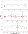 |
Fig. 13. Regions from 8040 to 8120 Å (top panel), 8415 to 8555 Å (middle panel), and 8620 to 8695 Å (bottom panel) of the HIRES Keck spectrum of EPIC 205375290: the observed spectrum is shown in black and the calculated synthetic spectrum with the final adopted parameters of Teff, of 3670 ± 180 K, and a log g of 3.85 ± 0.3 is shown in red. |
The accuracy of our determination of EPIC 205375290’s fundamental parameters (Table 5) is limited by several factors: (i) The spectrum only has a modest S/N of only ∼35. (ii) Numerous weak TiO lines are present in the spectrum which are not well described by the current atomic data, and therefore they introduce additional “noise”. (iii) The most important gravity indicators in M-type stars – the regions of the K I and red Na I doublets at 7664 Å and 7699 Å and 8183 Å and 8194 Å respectively – fell into inter-order gaps in the HIRES spectrum we used. Therefore, we used the wings of the Ca II lines as constraints for log g. (iv) Some of the spectral lines show a slight blueward asymmetry which could be an effect of the circumstellar environment or of a potential, yet unresolved binarity. Consequently, the derived fundamental parameters can only be used as a first estimate with relatively high errors. For a more detailed and more accurate analysis, a high-resolution, high S/N spectrum would be required and will hopefully be obtained in the future.
Fundamental parameters for EPIC 205375290 from high-resolution spectroscopy.
It is obvious that our spectroscopically determined values for Teff and log g place EPIC 205375290 below the line where νmax is equal to the Nyquist frequency of LC data in Fig. 11. Currently, we can only speculate about the origin of this discrepancy. One explanation is related to the above-mentioned high uncertainties of the spectroscopically determined fundamental parameters; in particular the log g value is likely overestimated. This discrepancy may also originate from the assumption that the scaling relation for stars that are on the main sequence or later is fully applicable to pre-MS stars in an inverse form, which might not be the case. Additional work is required to investigate this further, but this is out of the scope of the present analysis.
7. Conclusions
We have developed APOLLO, a software package based on DIAMONDS that uses a new Bayesian approach for the detection of low-S/N solar-like oscillations in the presence of a high background level. High background levels can, for example, originate from highly active stars, in particular in their earliest stages of evolution prior to the onset of core-hydrogen burning. For the search of solar-like oscillations in pre-MS stars, a reliable treatment of such high background levels is a crucial prerequisite.
In addition to the photometric time series obtained from space, APOLLO only requires the stars’ effective temperatures and magnitudes as input for the determination of the frequency of maximum power, νmax, and the large frequency separation, Δν. For any Bayesian method, good priors have to be selected. For this, APOLLO uses dedicated estimation algorithms which compute prior distributions for the ten parameters σb, a1, a2, a3, b1, b2, b3, Hosc, νmax, and σenv.
We tested our new method on 1071 confirmed solar-like oscillators observed by the Kepler satellite in long cadence; the majority of the objects have data from the full four years of Kepler observations. With these data, we calibrated APOLLO, and tested the reliability of our method. We then subsequently reduced the observation lengths to the time bases obtained with the TESS mission, which are 356.2 d, 109.6 d, 82.2 d, 54.8 d, and 27.4 d. As the observational time bases get shorter, the distributions of the νmax and Δν values get broader. But overall, we find that our method is robust even when shortening the observation length dramatically. Consequently, APOLLO can be applied to data observed by various current and future missions (e.g., TESS, Kepler K2 and in the future PLATO), and is designed such that it can process large amounts of observational data quickly and efficiently.
In a final step, we applied APOLLO to a sample of 135 candidate stars in the pre-MS stage observed in the K2 Campaign 2 on Upper Scorpius in long cadence. Most of the candidates have an expected νmax larger than the Nyquist frequency for K2 LC data, and no SC observations are available for these stars. Although this complicates our search, we identified a possible candidate for pre-MS solar-like oscillations, EPIC 205375290, which shows a power excess around a νmax of 242 ± 10 μHz, which we found to be statistically signifcant according to our Bayesian model comparison. For the verification of EPIC 205375290 as the first pre-MS solar-like oscillator additional work is required in the future: on the observational side longer photometric time series at shorter cadence and higher S/N ratio spectroscopic data are needed; on the theoretical side, whether or not the scaling relation used, which is usually applied to main sequence stars and later, can be applied in its inverse form for pre-MS solar-like oscillators needs to be tested.
Acknowledgments
E.C. is funded by the European Union’s Horizon 2020 research and innovation program under the Marie Sklodowska-Curie grant agreement No. 664931. A.K. acknowledges support from the National Research Foundation (NRF) of South Africa. I.P. was supported by budgetary funding of the Basic Research programme II.16. Some spectral data for this work were obtained with the Southern African Large Telescope (SALT) under program 2019-1-MLT-002.
References
- Alencar, S. H. P., Teixeira, P. S., Guimarães, M. M., et al. 2010, A&A, 519, A88 [NASA ADS] [CrossRef] [EDP Sciences] [Google Scholar]
- Anderson, E. R., Duvall, T. L., Jr., & Jefferies, S. M. 1990, ApJ, 364, 699 [NASA ADS] [CrossRef] [Google Scholar]
- Antoci, V., Handler, G., Campante, T. L., et al. 2011, Nature, 477, 570 [NASA ADS] [CrossRef] [PubMed] [Google Scholar]
- Appourchaux, T. 2014, A Crash Course on Data Analysis in Asteroseismology (Cambridge: Cambridge University Press), 123 [Google Scholar]
- Appourchaux, T., Chaplin, W. J., García, R. A., et al. 2012, A&A, 543, A54 [NASA ADS] [CrossRef] [EDP Sciences] [Google Scholar]
- Astropy Collaboration (Robitaille, T. P., et al.) 2013, A&A, 558, A33 [NASA ADS] [CrossRef] [EDP Sciences] [Google Scholar]
- Astropy Collaboration (Price-Whelan, A. M., et al.) 2018, AJ, 156, 123 [Google Scholar]
- Auvergne, M., Bodin, P., Boisnard, L., et al. 2009, A&A, 506, 411 [NASA ADS] [CrossRef] [EDP Sciences] [Google Scholar]
- Basri, G., & Batalha, C. 1990, ApJ, 363, 654 [NASA ADS] [CrossRef] [Google Scholar]
- Bastien, F. A., Stassun, K. G., Basri, G., & Pepper, J. 2013, Nature, 500, 427 [NASA ADS] [CrossRef] [PubMed] [Google Scholar]
- Behrend, R., & Maeder, A. 2001, A&A, 373, 190 [NASA ADS] [CrossRef] [EDP Sciences] [Google Scholar]
- Bell, K. J., Hekker, S., & Kuszlewicz, J. S. 2019, MNRAS, 482, 616 [NASA ADS] [CrossRef] [Google Scholar]
- Bonanno, A., Corsaro, E., & Karoff, C. 2014, A&A, 571, A35 [NASA ADS] [CrossRef] [EDP Sciences] [Google Scholar]
- Borucki, W. J., Koch, D., Basri, G., et al. 2010, Am. Astron. Soc. Meet. Abstr., 215, 101.01 [Google Scholar]
- Brown, T. M., Latham, D. W., Everett, M. E., & Esquerdo, G. A. 2011, AJ, 142, 112 [NASA ADS] [CrossRef] [Google Scholar]
- Buckley, D. A. H., Swart, G. P., & Meiring, J. G. 2006, SPIE Conf. Ser., 6267, 62670Z [Google Scholar]
- Bugnet, L., García, R. A., Davies, G. R., et al. 2018, A&A, 620, A38 [NASA ADS] [CrossRef] [EDP Sciences] [Google Scholar]
- Bugnet, L., García, R. A., Mathur, S., et al. 2019, A&A, 624, A79 [EDP Sciences] [Google Scholar]
- Burgh, E. B., Nordsieck, K. H., Kobulnicky, H. A., et al. 2003, in Instrument Design and Performance for Optical/Infrared Ground-based Telescopes, eds. M. Iye, & A. F. M. Moorwood (SPIE), Int. Soc. Opt. Photon., 4841, 1463 [NASA ADS] [CrossRef] [Google Scholar]
- Campante, T. L., Schofield, M., Kuszlewicz, J. S., et al. 2016, ApJ, 830, 138 [NASA ADS] [CrossRef] [Google Scholar]
- Chaplin, W. J., & Miglio, A. 2013, ARA&A, 51, 353 [Google Scholar]
- Chaplin, W. J., Bedding, T. R., Bonanno, A., et al. 2011, ApJ, 732, L5 [Google Scholar]
- Cody, A. M., Stauffer, J., Baglin, A., et al. 2014, AJ, 147, 82 [NASA ADS] [CrossRef] [Google Scholar]
- Colman, I. L., Huber, D., Bedding, T. R., et al. 2017, MNRAS, 469, 3802 [Google Scholar]
- Corsaro, E., & De Ridder, J. 2014, A&A, 571, A71 [NASA ADS] [CrossRef] [EDP Sciences] [Google Scholar]
- Corsaro, E., & De Ridder, J. 2015, Eur. Phys. J. Web Conf., 101, 06019 [Google Scholar]
- Corsaro, E., Fröhlich, H. E., Bonanno, A., et al. 2013, MNRAS, 430, 2313 [NASA ADS] [CrossRef] [Google Scholar]
- Corsaro, E., Mathur, S., García, R. A., et al. 2017, A&A, 605, A3 [NASA ADS] [CrossRef] [EDP Sciences] [Google Scholar]
- Cutri, R. M., Skrutskie, M. F., van Dyk, S., et al. 2003, VizieR Online Data Catalog: II/246 [Google Scholar]
- De Ridder, J., Barban, C., Baudin, F., et al. 2009, Nature, 459, 398 [Google Scholar]
- Dodin, A. V. 2015, Astron. Lett., 41, 196 [Google Scholar]
- Dodin, A. V., & Lamzin, S. A. 2012, Astron. Lett., 38, 649 [NASA ADS] [CrossRef] [Google Scholar]
- Duvall, T. L., Harvey, J. W., & Pomerantz, M. A. 1986, Antarct. J. US, 21, 280 [Google Scholar]
- Edwards, S., Hartigan, P., Ghandour, L., & Andrulis, C. 1994, AJ, 108, 1056 [NASA ADS] [CrossRef] [Google Scholar]
- Feroz, F., & Hobson, M. P. 2008, MNRAS, 384, 449 [NASA ADS] [CrossRef] [Google Scholar]
- Fröhlich, H. E., Frasca, A., Catanzaro, G., et al. 2012, A&A, 543, A146 [NASA ADS] [CrossRef] [EDP Sciences] [Google Scholar]
- García, R. A., & Ballot, J. 2019, Liv. Rev. Sol. Phys., 16, 4 [Google Scholar]
- Gilliland, R. L., Jenkins, J. M., Borucki, W. J., et al. 2010, ApJ, 713, L160 [NASA ADS] [CrossRef] [Google Scholar]
- Handberg, R., & Lund, M. N. 2014, MNRAS, 445, 2698 [Google Scholar]
- Handberg, R., & Lund, M. N. 2019, https://doi.org/10.5281/zenodo.2579846 [Google Scholar]
- Howell, S. B., Sobeck, C., Haas, M., et al. 2014, PASP, 126, 398 [NASA ADS] [CrossRef] [Google Scholar]
- Huber, D., Bedding, T. R., Stello, D., et al. 2011, ApJ, 743, 143 [Google Scholar]
- Huber, D., Bryson, S. T., Haas, M. R., et al. 2016, ApJS, 224, 2 [NASA ADS] [CrossRef] [Google Scholar]
- Jenkins, J. M., Caldwell, D. A., Chandrasekaran, H., et al. 2010, ApJ, 713, L120 [NASA ADS] [CrossRef] [Google Scholar]
- Kallinger, T., Mosser, B., Hekker, S., et al. 2010, A&A, 522, A1 [NASA ADS] [CrossRef] [EDP Sciences] [Google Scholar]
- Kallinger, T., De Ridder, J., Hekker, S., et al. 2014, A&A, 570, A41 [NASA ADS] [CrossRef] [EDP Sciences] [Google Scholar]
- Kallinger, T., Hekker, S., Garcia, R. A., Huber, D., & Matthews, J. M. 2016, Sci. Adv., 2, 1500654 [NASA ADS] [CrossRef] [Google Scholar]
- Karoff, C. 2012, MNRAS, 421, 3170 [NASA ADS] [CrossRef] [Google Scholar]
- Karoff, C., Campante, T. L., Ballot, J., et al. 2013, ApJ, 767, 34 [NASA ADS] [CrossRef] [Google Scholar]
- Kjeldsen, H., & Bedding, T. R. 1995, A&A, 293, 87 [NASA ADS] [Google Scholar]
- Kjeldsen, H., Christensen-Dalsgaard, J., Handberg, R., et al. 2010, Astron. Nachr., 331, 966 [NASA ADS] [CrossRef] [Google Scholar]
- Kobulnicky, H. A., Nordsieck, K. H., Burgh, E. B., et al. 2003, in Instrument Design and Performance for Optical/Infrared Ground-based Telescopes, eds. M. Iye, & A. F. M. Moorwood (SPIE), Int. Soc. Opt. Photon., 4841, 1634 [NASA ADS] [CrossRef] [Google Scholar]
- Koch, D. G., Borucki, W. J., Basri, G., et al. 2010, ApJ, 713, L79 [NASA ADS] [CrossRef] [Google Scholar]
- Lomb, N. R. 1976, Ap&SS, 39, 447 [Google Scholar]
- Luger, R., Agol, E., Kruse, E., et al. 2016, AJ, 152, 100 [Google Scholar]
- Luger, R., Foreman-Mackey, D., & Hogg, D. W. 2017, Res. Notes Am. Astron. Soc., 1, 7 [Google Scholar]
- Lund, M. N., Silva Aguirre, V., Davies, G. R., et al. 2017, ApJ, 835, 172 [Google Scholar]
- Mathur, S., Handberg, R., Campante, T. L., et al. 2011a, ApJ, 733, 95 [NASA ADS] [CrossRef] [Google Scholar]
- Mathur, S., Hekker, S., Trampedach, R., et al. 2011b, ApJ, 741, 119 [NASA ADS] [CrossRef] [Google Scholar]
- Michel, E., Baglin, A., Auvergne, M., et al. 2008, Science, 322, 558 [NASA ADS] [CrossRef] [PubMed] [Google Scholar]
- Mosser, B., Elsworth, Y., Hekker, S., et al. 2012, A&A, 537, A30 [NASA ADS] [CrossRef] [EDP Sciences] [Google Scholar]
- Oliphant, T. E. 2006, A Guide to NumPy (USA: Trelgol Publishing), 1 [Google Scholar]
- Palla, F., & Stahler, S. W. 1990, ApJ, 360, L47 [NASA ADS] [CrossRef] [Google Scholar]
- Pande, D., Bedding, T. R., Huber, D., & Kjeldsen, H. 2018, MNRAS, 480, 467 [NASA ADS] [CrossRef] [Google Scholar]
- Paxton, B., Bildsten, L., Dotter, A., et al. 2011, ApJS, 192, 3 [Google Scholar]
- Paxton, B., Cantiello, M., Arras, P., et al. 2013, ApJS, 208, 4 [NASA ADS] [CrossRef] [Google Scholar]
- Paxton, B., Marchant, P., Schwab, J., et al. 2015, ApJS, 220, 15 [Google Scholar]
- Paxton, B., Schwab, J., Bauer, E. B., et al. 2018, ApJS, 234, 34 [Google Scholar]
- Paxton, B., Smolec, R., Schwab, J., et al. 2019, ApJS, 243, 10 [Google Scholar]
- Pecaut, M. J., & Mamajek, E. E. 2016, MNRAS, 461, 794 [Google Scholar]
- Pinheiro, F. J. G. 2008, A&A, 478, 193 [EDP Sciences] [Google Scholar]
- Pinsonneault, M. H., Elsworth, Y., Epstein, C., et al. 2014, ApJS, 215, 19 [Google Scholar]
- Piskunov, N., & Valenti, J. A. 2017, A&A, 597, A16 [NASA ADS] [CrossRef] [EDP Sciences] [Google Scholar]
- Preibisch, T., Guenther, E., & Zinnecker, H. 2001, AJ, 121, 1040 [NASA ADS] [CrossRef] [Google Scholar]
- Rauer, H., Catala, C., Aerts, C., et al. 2014, Exp. Astron., 38, 249 [Google Scholar]
- Ricker, G. R., Vanderspek, R. K., Latham, D. W., & Winn, J. N. 2014, Am. Astron. Soc. Meet. Abstr., 224, 113.02 [Google Scholar]
- Samadi, R., Goupil, M. J., Alecian, E., et al. 2005, J. Astrophys. Astron., 26, 171 [Google Scholar]
- Sánchez-Blázquez, P., Peletier, R. F., Jiménez-Vicente, J., et al. 2006, MNRAS, 371, 703 [NASA ADS] [CrossRef] [Google Scholar]
- Savitzky, A., & Golay, M. J. E. 1964, Anal. Chem., 36, 1627 [Google Scholar]
- Scargle, J. D. 1982, ApJ, 263, 835 [Google Scholar]
- Schofield, M., Chaplin, W. J., Huber, D., et al. 2019, ApJS, 241, 12 [Google Scholar]
- Shaw, J. R., Bridges, M., & Hobson, M. P. 2007, MNRAS, 378, 1365 [NASA ADS] [CrossRef] [Google Scholar]
- Skilling, J. 2006, in Bayesian Inference and Maximum Entropy Methods in Science and Engineering, ed. A. Mohammad-Djafari, AIP Conf. Ser., 872, 321 [Google Scholar]
- Stassun, K. G., Corsaro, E., Pepper, J. A., & Gaudi, B. S. 2018, AJ, 155, 22 [NASA ADS] [CrossRef] [Google Scholar]
- Stello, D., Bruntt, H., Preston, H., & Buzasi, D. 2008, ApJ, 674, L53 [NASA ADS] [CrossRef] [Google Scholar]
- Stello, D., Chaplin, W. J., Basu, S., Elsworth, Y., & Bedding, T. R. 2009, MNRAS, 400, L80 [NASA ADS] [CrossRef] [Google Scholar]
- Trotta, R. 2006, in Statistical Problems in Particle Physics, Astrophysics and Cosmology, eds. L. Lyons, & M. Karagöz Ünel, 15 [Google Scholar]
- Valenti, J. A., & Piskunov, N. 1996, A&AS, 118, 595 [NASA ADS] [CrossRef] [EDP Sciences] [Google Scholar]
- Valenti, J. A., Piskunov, N., & Johns-Krull, C. M. 1998, ApJ, 498, 851 [Google Scholar]
- Virtanen, P., Gommers, R., Oliphant, T. E., et al. 2020, Nat. Meth., 17, 261 [Google Scholar]
- Walker, G., Matthews, J., Kuschnig, R., et al. 2003, PASP, 115, 1023 [NASA ADS] [CrossRef] [Google Scholar]
- White, R., & Basri, G. 2003, in Brown Dwarfs, ed. E. Martín, IAU Symp., 211, 143 [Google Scholar]
All Tables
Empirical scale for comparison of the strength of evidence to determine the Bayes factor (Trotta 2006).
All Figures
|
Fig. 1. Upper panel: values for νmax extracted from the FliPer method as compared to the values from the APOKASC catalogue. Lower panel: corresponding residuals as percentile. The red shaded area represents the uncertainties in the catalogue. The blue shaded areas define our 1-σ interval, centred around νmax from FliPer. |
| In the text | |
|
Fig. 2. Distribution of values for νmax extracted from the FliPer method. The Y axis shows the percentage of values within a given bin of deviation from a corresponding literature value, while the X axis shows the deviation from the literature value in percent. The distribution can be represented by a Gaussian function, whose fit to the histogram is represented by a dotted green line. The mean for this distribution is at 4.95%, with a standard deviation of 6.93%. For visualisation purposes, deviations above 30% and below −30% are excluded. |
| In the text | |
|
Fig. 3. fIT provided by DIAMONDS for three different observation lengths for KIC 9903915. Upper row: full background model, lower row: noise only model. Different observation lengths are split into three columns: first column: result for the full 1400 day light curve, second: for 109.6 days and third: for 27.4 days. We find strong evidence for all three observation lengths: log O = 990.53 for 1400 days, and log O = 75.42 and log O = 13.86 for 27 days. Even at 27 days we are still above the threshold of log O = 5 for strong evidence. |
| In the text | |
|
Fig. 4. Resulting νmax, APOLLO values of the APOLLO pipeline in relation to catalogue values of our red-giant sample. Upper panel: comparison of νmax, APOLLO to the literature, with the red shaded area illustrating the 1-σ uncertainties in the literature. Lower plot: residuals in sigma of the literature value and again mark the uncertainties in the red shaded area. |
| In the text | |
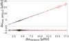 |
Fig. 5. Similar as Fig. 4, but for the large frequency separation Δν. |
| In the text | |
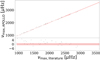 |
Fig. 6. Similar to Fig. 4 but for the sample from the LEGACY catalogue. |
| In the text | |
|
Fig. 7. Distribution of values for νmax (left panel) and Δν (right panel) in different observation lengths. Grey filled bars represent the values for 1400 days of observation, and smaller observation lengths are shown in different colours. The red dashed lines represent the 1-σ range of the literature values. The legend states the percentage value of stars within 1-σ. In brackets we note the percentage value when taking the uncertainties of the fit into account. For νmax, using 27 d observations 19.88% of our sample falls outside of the 1-σ range in comparison to the full observation length. For Δν this decrease is much stronger, with 83.91% of the sample falling outside of 1-σ using 27 d of observation. |
| In the text | |
|
Fig. 8. Relation between Kepler magnitude Kp, and white noise. The black solid line represents the relation from Pande et al. (2018), the grey shaded area represents the white noise range corresponding to a variation of 0.4 mag. Our sample is represented by the grey and red dots, where the red dots constitute the sample used in the magnitude analysis, and is identified by the intersection of the horizontal lines with the grey shaded area. The horizontal grey dashed lines show the range of these points within 11.6 mag < Kp < 12 mag. |
| In the text | |
|
Fig. 9. Relation between Bayes factor Oosc, noise and Kepler magnitude as well as the converted TESS magnitude. Different observation lengths are color coded. |
| In the text | |
|
Fig. 10. Relation between Bayes factor Oosc, noise and Kepler magnitude for the main sequence sample. |
| In the text | |
|
Fig. 11. Evolutionary tracks in a log Teff − log g diagram. The colour code describes νmax obtained from the scaling relation. The black line shows the location at which νmax is equal to the Nyquist frequency of LC data. The red and blue lines show the locations of the birthline according to Palla & Stahler (1990) and Behrend & Maeder (2001), respectively. The black crossed object shows the spectroscopic observations for EPIC 205375290. |
| In the text | |
|
Fig. 12. Upper panel: resulting fit for EPIC 205375290. In dashed blue are the Harvey-like functions, the dotted cyan line shows the power excess, the yellow dotted line the white noise, and the red solid line the full fit of the oscillation model. The green line represents a smoothed variant of the PSD. Lower panel: light curve of EPIC 205375290. The filtered and reduced light curve used for the analysis is shown in black while the original light curve is shown in red. |
| In the text | |
|
Fig. 13. Regions from 8040 to 8120 Å (top panel), 8415 to 8555 Å (middle panel), and 8620 to 8695 Å (bottom panel) of the HIRES Keck spectrum of EPIC 205375290: the observed spectrum is shown in black and the calculated synthetic spectrum with the final adopted parameters of Teff, of 3670 ± 180 K, and a log g of 3.85 ± 0.3 is shown in red. |
| In the text | |
Current usage metrics show cumulative count of Article Views (full-text article views including HTML views, PDF and ePub downloads, according to the available data) and Abstracts Views on Vision4Press platform.
Data correspond to usage on the plateform after 2015. The current usage metrics is available 48-96 hours after online publication and is updated daily on week days.
Initial download of the metrics may take a while.