| Issue |
A&A
Volume 647, March 2021
|
|
|---|---|---|
| Article Number | A39 | |
| Number of page(s) | 28 | |
| Section | Galactic structure, stellar clusters and populations | |
| DOI | https://doi.org/10.1051/0004-6361/202038840 | |
| Published online | 05 March 2021 | |
Towards a fully consistent Milky Way disk model
IV. The impact of Gaia DR2 and APOGEE
Astronomisches Rechen-Institut, Zentrum für Astronomie der Universität Heidelberg, Mönchhofstr. 12–14, 69120 Heidelberg, Germany
e-mail: Sysoliatina@uni-heidelberg.de
Received:
3
July
2020
Accepted:
1
December
2020
Aims. We present an updated version of the semi-analytic Just-Jahrei (JJ) model of the Galactic disk and constrain its parameters in the Solar neighbourhood.
Methods. The new features of the JJ model include a simple two-component gaseous disk, a star-formation rate (SFR) function of the thick disk that has been extended in time, and a correlation between the kinematics of molecular gas and thin-disk populations. Here, we study the vertical number density profiles and W-velocity distributions determined from ∼2 × 10⁶ local stars of the second Gaia data release (DR2). We also investigate an apparent Hess diagram of the Gaia DR2 stars selected in a conic volume towards the Galactic poles. Using a stellar evolution library, we synthesise stellar populations with a four-slope broken power-law initial mass function, the SFR, and an age-metallicity relation. The latter is consistently derived with the observed metallicity distribution of the local Red Clump giants from the Apache Point Observatory Galactic Evolution Experiment (APOGEE). Working within a Bayesian approach, we sample the posterior probability distribution in a multidimensional parameter space using the Markov chain Monte Carlo method.
Results. We find that the spatial distribution and motion of the Gaia DR2 stars imply two recent SF bursts centered at ages of ∼0.5 Gyr and ∼3 Gyr and characterised by a ∼30% and ∼55% SF enhancement, respectively, relative to a monotonously declining SFR continuum. The stellar populations associated with this SF excess are found to be dynamically hot for their age: they have W-velocity dispersions of ∼12.5 km s−1 and ∼26 km s−1. The new JJ model is able to reproduce the local star counts with an accuracy of ∼5%.
Conclusions. Using Gaia DR2 data, we self-consistently constrained 22 parameters of the updated JJ model. Our optimised model predicts two SF bursts within the last ∼4 Gyr, which may point to recent episodes of gas infall.
Key words: Galaxy: disk / Galaxy: kinematics and dynamics / solar neighborhood / Galaxy: evolution
© ESO 2021
1. Introduction
Our current understanding of the morphology and kinematics of the Milky Way, and of the physical processes that shape its structure and govern its evolution, is deepening to a greater extent and faster than ever. Since the second data release of the astrometric mission Gaia in April 2018 (DR2, Gaia Collaboration 2016, 2018a), many new details on Galactic morphology have been revealed by studies based on the high-precision Gaia astrometry, in addition to studies of the data from the available high-resolution and large spectroscopic surveys, such as the Sloan Digital Sky Survey (SDSS), Apache Point Observatory Galactic Evolution Experiment (APOGEE, Eisenstein et al. 2011; Majewski et al. 2017), the Galactic Archaeology with HERMES (GALAH, Martell et al. 2017), and The Large Sky Area Multi-Object Fibre Spectroscopic Telescope Survey (LAMOST, Cui et al. 2012). At the same time, many of the previously known properties of the Galaxy have been re-confirmed and investigated to a much greater extent than ever before.
A number of studies of local kinematics with Gaia DR2 have reported the presence of numerous arc-like substructures in the velocity space (Vr, Vϕ)1 (Gaia Collaboration 2018b; Hunt et al. 2019; Khanna et al. 2019). These kinematic signatures of the local stellar streams and moving groups are qualitatively reproduced in N-body simulations with a transient spiral structure in the presence of a bar (Hunt et al. 2019; Khanna et al. 2019). Another example is a newly discovered ‘phase spiral’ in the (Vz,z) space, whose origin may be related to external perturbations (Bland-Hawthorn et al. 2019) or the secular disk evolution (Khoperskov et al. 2019). These kinematic features give us strong evidence of ongoing phase mixing processes in the present-day Galaxy, implying that the latter is currently out of an equilibrium state. Another non-equilibrium feature was found by Bennett & Bovy (2019), who examined the south-north asymmetries in the vertical star count and kinematic trends in the Solar neighbourhood. The authors found a wave-like plane-asymmetric pattern both in star counts and stellar kinematics; as they are similar for all stellar populations, these waves may be a disk response to the recent interaction with a satellite since such disk-satellite interactions have been predicted to excite bending and breathing modes in the disk (Widrow et al. 2014).
Additionally, many new stellar aggregates are identified in the Gaia DR2 data. Meingast et al. (2019) detected a local stream located within 400 pc from the Sun that consists of dynamically cold stars with a three-dimensional (3D) velocity dispersion of only 1.3 km s−1. New catalogues of OB stars and open clusters (Cantat-Gaudin & Anders 2020; Chen et al. 2019; Liu & Pang 2019) allow for a better tracing of the Milky Way spiral pattern. The extensive samples of Gaia DR2 A- and F-type stars, as well as lower main-sequence (MS) stars, were used to test the plausibility of the different formation scenarios of spiral arms in the Galaxy (Griv et al. 2020). Also, the five-dimensional (5D) dynamic information from Gaia DR2 revealed mostly young filamentary stellar groups in the Solar neighbourhood that reflect the last ∼1 Gyr of star formation (SF) in the disk (Kounkel & Covey 2019).
These examples clearly show that the Gaia data reveal the most realistic picture of the Milky Way that has ever been available to astronomers. This new, complex picture enables us to expand our knowledge of the Galaxy formation and evolution. However, despite of the abundance of this new observational information, recent years yielded relatively few studies attempting to reconstruct the global star-formation rate (SFR) and the dynamic evolution of the Milky Way. With our present-day understanding of the complexity of the physical processes guiding Galactic evolution, the task of building a concordance model of the Milky Way seems more challenging than ever.
Many modern semi-analytic Milky Way models derive the Galactic gravitational potential self-consistently with the assumed matter distribution, based on the combined Poisson-Boltzmann equation. The first model of this class described the Solar neighbourhood in terms of a multicomponent disk consisting of a set of isothermal stellar populations in the presence of a spheroidal halo (Bahcall 1984). By introducing a parametrised SFR, a disk heating function in the form of an age-velocity dispersion relation (AVR), as well as an initial mass function (IMF) and an age-metallicity relation (AMR), we can then fully constrain the local disk evolution and predict the observed star counts. When applied to the different radial disk zones independently, this approach allows us to build a global model of the Galaxy. In such a way, for example, a multicomponent disk is described in the Besançon Galaxy model (BGM, Robin et al. 2003, 2012, 2017; Czekaj et al. 2014; Bienaymé et al. 2018). The BGM is widely used in a variety of Galactic studies. Ban et al. (2016) used the model to constrain the distribution of free-floating planets towards the Galactic centre (GC). Cabral et al. (2019) relied on the BGM stellar population synthesis to derive the chemical composition of the planetary building blocks. In comparison with the large-scale surveys, BGM was used to constrain the IMF, local SFR, and matter density (Mor et al. 2018) and proved helpful in studies of the disk formation (Robin et al. 2016; Nasello et al. 2018). It was also used to create a mock stellar catalogue at the preparatory step to Gaia DR2 (Rybizki et al. 2018). Thus, such Galactic models built of independent radial zones are handy tools that allow us to investigate key aspects of the evolution of the Milky Way.
However, there is a growing store of evidence indicating that different radial zones of the disk may actively interact with each other during its evolution history. For example, works based on the exploration of the disk metallicity gradient (Wielen et al. 1996), elemental abundances of the local interstellar medium (ISM), and young stars (Nieva & Przybilla 2012), as well as local kinematics (Sellwood & Binney 2002; Schönrich & Binney 2009), suggest that the Sun might have migrated from the inner disk up to several kpc during its 4.5 Gyr lifetime. There are two types of processes that can cause radial redistribution of the stars of the disk. Firstly, gravitational scattering leads to the diffusion of orbits in phase space, which is often referred as blurring. Secondly, stars may resonantly interact with non-axisymmetric disk structures, such as the bar and spiral arms. Resonant interactions mainly result in quick changes of orbital radii with essentially no change in eccentricity – this is referred to as the churning mechanism. Unfortunately, the relative weights of the two processes as well as their overall importance in disk evolution still remain highly uncertain. The spatial resolution of modern hydrodynamic simulations of Milky Way-like galaxies does not yet allow for the tracing of these processes in the disk and, therefore, radial migration cannot be unambiguously quantified from the theoretical point of view. Several attempts have been made to constrain radial migration based on reasonable assumptions about the disk evolution and the observed present-day metallicity distributions across the disk (Minchev et al. 2018; Frankel et al. 2018, 2020). They report a strong radial migration across the Galactic disk: for example, according to Frankel et al. (2020), 32% of 6 Gyr old stars will migrate more than 2.6 kpc from their birthplace. However, these studies rely on uncertain stellar ages, which may suffer from systematic errors, and they use a number of assumptions that are known to be simplifications or that may not necessarily be valid (e.g. ISM enrichment due to stellar evolution takes place at the stellar birthplace; SFR shape is exponentially declining).
At the moment, there is no global Milky Way model that is able to predict the detailed radial and vertical disk structure, incorporate stellar evolution to produce star counts, and simultaneously take into account the radial migration. Indeed, adding the radial migration mechanisms in their parametrised form to a BGM-like model adds a significant level of complexity to the whole machinery of a stellar population synthesis: the AMR can no longer be used as an input, but instead, a full chemical evolution model must be added to predict the ISM composition at each radius and each moment of time. We would also have a number of additional free parameters to be constrained, which cannot be done based solely on the local data, requiring instead an extended data sample. In practice, the radial migration is often ignored in Galactic studies, such that the results derived from the data covering some range of Galactocentric distances can be interpreted as ‘averaged’ due to migration over a larger distance range.
Some of the above-mentioned observational evidence from Gaia DR2 suggests that the Milky Way experienced disk-satellite interaction episodes that left imprints on the spatial distribution and kinematics of its stars. At the same time, disk-satellite interactions are expected to have an impact on the SFR, both through the direct accretion of gas and stars from the impactor and by triggering SF processes in the disk by tidal forces and shocks. Therefore, it is plausible that the Milky Way’s SFR would exhibit measurable deviations from a simple exponential or power-law decline during the last ∼8 Gyr. With these considerations taken into account, Mor et al. (2019) used ∼2.9 × 10⁶Gaia DR2 stars over the Hess diagram to constrain the Galactic SFR. The SFR was given in a non-parametric form in nine age bins in the framework of BGM. As the SFR cannot be disentangled from the IMF, they also varied the slopes of the three-slope broken power-law IMF. As a result, Mor et al. (2019) found that the data demonstrate an excess of young A and F stars with respect to models having an exponentially declining SFR, such that their best model includes a SF burst 2−3 Gyr ago. However, the obtained constraints on the burst shape and position are not very strong and, in principle, a model with almost constant SFR with a quick drop during the last ∼1 Gyr cannot be ruled out either. Also, the authors did not check the consistency between the observed kinematics and the dynamic heating prescribed by the BGM. In addition, the assumed dynamical heating of the disk has its own impact on the predicted star counts and should, therefore, also be adapted to obtain robust SFR parameters.
These findings motivated us to put a reliable constraint on the shape of the thin-disk SFR using our local semi-analytic disk model. In this study, we aim to optimise the SFR self-consistently not only with the IMF, but also with the AVR and AMR functions. In previous papers of this series, we presented a semi-analytic Just-Jahreiß disk model (JJ model hereafter). The model describes the thin disk as a set of isothermal mono-age populations whose evolution is represented by four input functions given in analytic form: SFR, IMF, AVR, and AMR. The thick disk, gas, dark matter (DM), and stellar halo are also added to the total mass budget. The model is based on an iterative solving of the Poisson-Boltzmann equation in a thin-disk approximation. The JJ model does not aim to reproduce the south-north and azimuth asymmetries in the local disk structure and kinematics, but traces the overall trends in stellar spatial distribution, vertical kinematics, and metallicity gradients averaged over large enough volumes. This approach allows to keep the number of model parameters relatively small and, at the same time, to describe the main properties of the chemical, stellar, and dynamic evolution of the disk.
In Just & Jahreiß (2010, hereafter Paper I), the kinematic parameters of the JJ model were calibrated against the vertical kinematics of the HIPPARCOS MS stars (van Leeuwen 2007), which were complemented with the sample taken from the Fourth Catalogue of Nearby Stars (CNS4, Jahreiß & Wielen 1997). Additionally, F and G stars from the Geneva-Copenhagen Survey (GCS1, Nordström et al. 2004) were used to constrain the AMR shape. In Just et al. (2011, Paper II), the SFR and thick-disk parameters were constrained via calibration against the SDSS star counts in the cone towards the northern Galactic pole. Their best fit corresponded to the thin-disk SFR monotonously declining after a peak ∼10 Gyr ago and to the thick-disk vertical density profile close to the sechα law of an isothermal stellar population. The IMF parameters were optimised with the local HIPPARCOS data combined with an updated version of the CNS4 (Rybizki & Just 2015, Paper III). The latest version of the model IMF is a four-slope broken power-law function (Rybizki 2018). Recently, the JJ model was tested in the Solar cylinder against the sample of stars selected from the fifth release of the Radial Velocity Experiment (RAVE DR5, Kunder et al. 2017) and the Tycho-Gaia Astrometric Solution catalogue (Lindegren et al. 2016) of the first Gaia data release (DR1, Gaia Collaboration 2016). This helped to identify a number of non-critical, albeit non-negligible, model-to-data discrepancies (Sysoliatina et al. 2018a).
As we showed in Sysoliatina et al. (2018a), a forward modelling approach with the reddening and distance errors included in the model makes the model-to-data comparison challenging and computationally expensive. Therefore, to perform an efficient exploration of the multidimensional parameter space for this study, we chose a Bayesian approach and sampled the posterior probability distribution with the Markov chain Monte Carlo (MCMC) method. To optimise model parameters, we use essentially complete Gaia DR2 data samples selected in the local volume with simple colour-magnitude cuts and corrected for the reddening and extinction with the 3D extinction maps from Lallement et al. (2018) and Green et al. (2019). We adapt the local surface density normalisations for all Galactic components, IMF and AVR parameters, as well as a set of parameters governing the shape of SFR. The latter is allowed to have two additional peaks at ages ≲4 Gyr. Each of them is characterised by a vertical velocity dispersion that is independent from the value prescribed by the AVR function for the thin-disk populations of the same age. The model-to-data comparison is performed in terms of the vertical number density profiles of different stellar populations, their velocity distribution functions, and an apparent Hess diagram. We additionally use the APOGEE Red Clump (RC) sample to constrain the local AMR and then keep it constant during the MCMC posterior probability distribution sampling. This two-step update of parameters is possible because the chemical enrichment history has only a small impact on the predicted star counts and disk kinematics and, therefore, the AMR parameters can be updated post factum. A closure iteration over the AMR reconstruction procedure is performed in the end to achieve a full consistency between the dynamic and chemical parts of the model.
We note here that as we are currently modelling only the Solar neighbourhood and working solely with the local data, and also due to the difficulty in quantifying the radial migration processes, we do not add complexity to the JJ model by adding the radial migration. Instead, we keep in mind that the local data used for our analysis (and therefore our derived model parameters) partly represent other disk radial zones than just the local. In other words, the lack of the radial migration in the model affects the interpretation of its functions that describe the disk evolution. Our model SFR can be viewed as the present-day age distribution corrected for stellar evolution and averaged over R⊙ ± ΔR, where ΔR depends on the strength of the radial migration and may be as large as several kpc. The same interpretation is applicable to the heating function AVR and a simple chemical enrichment model in the form of the AMR.
This paper has the following structure. Section 2 describes the construction of the local Gaia DR2 samples of different stellar populations, as well as our selection of the local APOGEE RC sample. Section 3 presents a summary of the improvements introduced to the model. Section 4 describes the stellar population synthesis procedure and explains our parameter optimisation method. Section 5 contains the results of the MCMC posterior sampling. Then we discuss the obtained results in Sect. 6 and present our conclusions in Sect. 7. Additional material on Gaia DR2 TAP queries, the full posterior probability distribution, and an estimate of the impact of the 3D extinction maps on the data selection are presented in Appendices A–C.
2. Data
In order to improve the JJ model, which provides a detailed insight into the spatial structure and vertical kinematics of the Galactic disk in the Solar neighbourhood (Sect. 3), we require a local stellar sample with the full 6D dynamical information available. Moreover, these data have to be representative for the overall underlying distribution of stellar populations; alternatively, the data selection function has to be well understood. There is no doubt that the best data of this kind that is presently available comes from Gaia DR2 (Gaia Collaboration 2018a), with its high-quality astrometric, photometric, and spectroscopic measurements. Therefore, we chose Gaia DR2 as a base for our analysis of the spatial distribution and motions of the local stellar populations. The procedure is as follows.
First, we define our samples with simple colour-magnitude and distance cuts to build essentially complete samples of the local stars. With these criteria, we select Gaia DR2 stars with three known components of phase space (i.e. spatial coordinates) and use them to construct the vertical number density profiles. To study the vertical velocity distributions, we further select subsets with known proper motions and radial velocities. Our data selection procedure also includes astrometric and photometric quality cuts, de-reddening, and correction for the incompleteness of the selected samples.
Additionally, we use spectroscopic information from the APOGEE RC catalogue (Bovy et al. 2014), which provides a well-defined and mostly unbiased sample of bright stars across the Galactic disk. We use APOGEE RC robust distances, metallicities, and α-element abundances to constrain the chemical evolution of the disk in terms of the AMR (Sect. 4.5); in the next step, this simple chemical enrichment model is applied to perform a stellar population synthesis for the local volume.
2.1. Gaia samples
2.1.1. Absolute CMD
A detailed understanding of data completeness is critical for their adequate modelling and, thus, for improving model parameters. Therefore, before starting the data selection procedure, we thoughtfully address this question and then use our understanding of data completeness as our first guide to formulating reasonable sample selection criteria.
As presented in Gaia Collaboration (2018a), Gaia DR2 is expected to be essentially complete in the apparent magnitude range of 12 mag < G < 17 mag. At the very bright end, G ≲ 4 mag, star counts are known to be unreliable because of image saturation effects, but for stars with an apparent brightness of 7 mag ≲ G < 12 mag, the catalogue completeness is significantly improved in Gaia DR2 with respect to DR1 (see Fig. 1 in Gaia Collaboration 2018a). An estimate of the Gaia DR2 completeness was recently derived as a result of its comparison to the Two Micron All Sky Survey (2MASS, Skrutskie et al. 2006) and implemented in the Python module gdr2_completeness2. Gaia DR2 and 2MASS star counts were compared in three G-magnitude bins; this comparison shows that only when stars as faint as G ≈ 17−18 mag enter the sample, Gaia DR2 completeness starts to suffer in the near-plane regions, especially in the direction towards the GC, where completeness deteriorates due to strong extinction and stellar crowding. Even though in this case Gaia DR2 completeness can be as low as ∼70% for certain lines-of-sight, its typical value in the Galactic plane still remains as high as ∼95%.
Taking this information into account, together with the fact that the local stars predominantly appear to be intrinsically bright because of their proximity to the Sun, we decided to aim at local stars with apparent magnitudes in the range of 7 mag < G < 17 mag. This selection allows us to construct abundant local samples that include both bright and faint stars and, at the same time, to simplify the sample incompleteness modelling by assuming that the raw data retrieved from the Gaia DR2 catalogue are essentially complete.
To constrain properties of the stellar populations in a robust way, both young and old stars must be represented in the data. Therefore, our data selection criteria are additionally motivated by our pre-knowledge about age distributions of different stellar classes. For this reason, we targeted several areas of the colour-magnitude diagram (CMD) constructed with the Gaia GBP − GRP colours and absolute magnitudes MG. The latter are calculated from Gaia apparent magnitudes G and parallax distances and are de-reddened with the local 3D extinction map (Sects. 2.1.2 and 2.1.3, and also Appendix B). The six samples that we target through the simple colour-magnitude cuts (columns MG and GBP − GRP in Table 1, see also Fig. 2) can be classified into the following three groups according to their age coverage:
Data selection criteria and the Gaia DR2 sample statistics.
Young stars. They are represented by A and F samples. A-type stars trace the last ∼1 Gyr of the SF processes in the Galactic disk, and F stars have ages younger than ∼6 Gyr with a peak at ∼3.5 Gyr ago (see modelled age distributions of the samples in Fig. 8).
Old stars. We selected three MS samples that contain G and K dwarfs, as well as a mixture of both. These samples cover a full range of stellar ages and are dominated by old long-lived stars (50% of G and K dwarfs are older than ∼8 Gyr and ∼9 Gyr, respectively).
Mixed ages. Additionally, we used a sample of giants selected in a colour-magnitude range dominated by the RC stars. This sample of bright giants consists of a mixture of stars of different ages spanning over almost the whole age range, τ ≳ 0.5 Gyr. The RC stars are known to include a significant fraction of young stars, with their age distribution showing a strong peak at ∼1.5−2 Gyr.
2.1.2. Spatial geometry
As a next step, for each sample defined on the CMD, as given in Table 1, we use our adopted absolute and apparent magnitude limits to transform them to the limiting heliocentric distances:

This defines a spherical shell with the inner and outer radii of dmin and dmax, respectively, where a stellar population limited by the absolute magnitudes [MG, min, MG, max] falls into the range of apparent magnitudes [Gmin, Gmax] (Fig. 1). By setting Gmin and Gmax to the adopted boundaries of the Gaia DR2 completeness range of 7 mag and 17 mag, respectively, we built a set of essentially complete samples in the Solar neighbourhood. As we can see from Eq. (1), for many of our samples from Table 1, the outer radius of the shell dmax can be as large as ∼2 kpc. However, the median relative parallax error of the Gaia DR2 stars with 7 mag < G < 17 mag is as high as ∼10% at 2 kpc from the Sun. In this case, the inverse parallax is not a robust estimate of the true distance. In order to stay on the safe side, we set an absolute limit to dmax of 600 pc, as at this distance scale Gaia DR2 stars of 7 mag < G < 17 mag have median relative parallax errors of ≲2.5% only and, thus, our use of parallax distances is justified (see also Sect. 6.1.2).
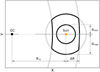 |
Fig. 1. Spatial geometry of the Gaia samples in XY projection (apart from the conic sample; see Sect. 2.1.5). The Galactic centre (GC) is marked with a black point. Each Gaia sample is selected in a Solar-centred spherical shell with the inner and outer radii of dmin and dmax from Table 1 (see columns d3 and d6 for the full samples and kinematic subsamples, respectively). Additionally, only stars belonging to the local annulus R⊙ ± ΔR with R = 8.2 kpc and ΔR = 150 pc are taken into consideration (thick grey arcs). |
Furthermore, we keep our samples very local in terms of Galactocentric distances in order to avoid interference on the part of the radial variations of the disk density and dynamical heating with parameters of the local JJ model. Thus, we selected only stars with Galactocentric distances R⊙ − ΔR < R < R⊙ + ΔR, where ΔR = 150 pc (Fig. 1). Galactocentric distances are calculated from parallax distances with the adopted Solar position at R⊙ = 8.2 ± 0.05 kpc (consistent with the most recent value of 8.178 ± 0.013stat ± 0.022sys kpc from Gravity & Abuter 2019) and z⊙ = 20 ± 3 pc (motivated by the value of 20.8 ± 0.3 pc from Bennett & Bovy 2019).
2.1.3. Reddening, quality cuts, and completeness
We calculate de-reddened magnitudes and colours using the local 3D dust map from Green et al. (2019). As it covers only about 3/4 of the sky, we complement it with the lower-resolution map from Lallement et al. (2018) to cover the remaining sky area (Fig. B.1). To calculate the colour excess EBP − RP and extinction AG, we use the colour transformations from Evans et al. (2018). The impact of the extinction and reddening on our sample statistics is discussed in Sect. 6.1.4 and Appendix B.
Additionally, we apply two cleaning cuts to remove stars with potentially unreliable astrometric and photometric parameters (based on discussions in Lindegren et al. 2018 and Evans et al. 2018):


The first cut cleans our data of astrometric binaries and the second one removes stars whose photometry was affected by saturation effects in the crowded fields. As these stars are real astrophysical objects, we add an additional correction to include the correct local mass and gravitational potential in the model. Together, these cuts remove up to ∼5% from our samples. The final number of stars in each sample is given in column 𝒩3 of Table 13. Column 𝒩3|no qual. contains the number of stars in the samples before the cleaning cuts were applied. We find that for all samples the astrometric quality cut, Eq. (2), is the main contributor to the fraction of removed stars. The incompleteness introduced by applying Eqs. (2) and (3) can be calculated simply as a ratio:
The left panel of the top row in Fig. 2 shows the absolute CMD of the final clean samples with three known components of phase space (i.e. the coordinate vector). The middle and right plots of the top row illustrate how the completeness factor 𝒮3 varies across the CMD and over the sky for each sample. In line with our expectations, the lowest completeness on the CMD have areas below the MS where binaries with a white dwarf companion can be located but a very low number of single MS stars. We also see a weak correlation between the completeness value and Galactic latitude, with the lower completeness area aligned with the Galactic plane. We compensate for the introduced incompleteness in a natural way, which also saves us computational time as is has to be applied only once: each star in a given sample is assigned with a weight 1/𝒮3(l, b), where 𝒮3(l, b) is completeness over the sky as shown at the top right panel of Fig. 2. These weights are later used during calculation of the observed number density profiles of the Gaia samples.
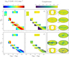 |
Fig. 2. Top row: selected samples of the local A, F, and RC stars and G and K dwarfs on the absolute CMD constructed with the de-reddened Gaia DR2 colours and magnitudes (left). Completeness of these samples as given by Eq. (4) over the CMD (middle) and across the sky (right). Bottom row: kinematic subsamples selected from the samples from the top row, except for A stars (left). Illustration of an additional incompleteness introduced by selecting only stars with available radial velocities (see Eq. (5)) and variation of this incompleteness over the CMD (middle) and across the sky (right). |
To study the disk kinematics we also need velocities, therefore we additionally use the Gaia DR2 7.2-million radial velocity catalogue (RVC, Katz et al. 2019). In practice, this means that we select subsets with known radial velocities from our previously defined colour-magnitude samples. So far, radial velocities have been measured by Gaia for relatively bright stars only, G ≲ 12−13 mag. Thus, our kinematic subsets are naturally restricted to have a faint limit around this value, we set Gmax = 12 mag. As for the bright apparent magnitude limit, we use the same value as before, namely, Gmin = 7 mag. In consequence, our kinematic samples occupy smaller volumes than the full colour-magnitude samples (compare their dmax values in Table 1, columns d3 and d6; also see Fig. 3). There is an additional limitation related to the stellar effective temperatures: RVC includes stars with temperatures up to 6900 K only. As a result, stars of spectral class A are completely missed in the RVC being too hot. In the case of the K-dwarf sample, we additionally clean the data from the core members of the Hyades cluster (Röser et al. 2019). For the stars in our remaining five kinematic subsamples, we calculate the vertical component of the spatial velocity, W, using the corresponding component of the Solar peculiar velocity W⊙ = 7.25 km s−1 (Schönrich et al. 2010). We also calculate W-velocity errors taking into account the full error covariance matrix provided in Gaia DR2.
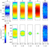 |
Fig. 3. Spatial distribution of the six Gaia samples (top row) and their five kinematic subsets (bottom row) plotted in XZ Cartesian coordinates. The X axis points to the GC. |
In order to ensure that these RVC subsamples (column 𝒩6 in Table 1) are kinematically unbiased, we estimate their completeness relative to the complementary samples built from stars with only three phase-space components known. For each kinematic subsample 𝒩6 we select stars from the corresponding final colour-magnitude sample 𝒩3 with apparent magnitudes G < 12 and stars that are located withing the volume of the kinematic subsample (column 𝒩3|G < 12 & d6 in Table 1). The overall completeness of the radial velocity samples ranges from ∼70% for F stars to ∼99% for the RC sample and is expressed as:
The left panel of the bottom row in Fig. 2 shows the logarithmic number density of the final kinematic subsamples at the absolute CMD. The corresponding middle and right panels illustrate the variation of the factor 𝒮v over the CMD and across the sky. The lowest completeness is seen near the Galactic plane and in the direction towards the GC. The completeness factor is essentially homogeneous over given areas of the absolute magnitudes and colours, except for the regions above the MS where binary stars are located. The correction of this incompleteness is performed exactly in the same way as in the case of their parent samples: weights 1/𝒮6(l, b) are used during the calculation of velocity distribution functions from the kinematic subsamples (Sect. 4). Figure 3 shows the spatial distribution in XZ projection of both full A-, F-, RC-star and G-, G/K-, K-dwarf samples (top row), and their kinematic subsamples (except of A stars, bottom row).
2.1.4. Full local sample
For subsequent testing of the updated JJ model (Sect. 5.3.4), we also use the full local sample consisting of all stars with apparent magnitudes 7 mag < G < 17 mag, colours 0 mag < GBP − GRP < 3 mag, and absolute magnitudes −2 mag < MG < 12 mag (Table 1). The full sample is selected in the local 600-pc sphere truncated by the cut R⊙ − ΔR < R < R⊙ + ΔR with ΔR = 150 pc, as before. The quality cuts from Eqs. (2) and (3), as well as de-reddening, are applied in the full analogy to the colour-magnitude samples described above.
2.1.5. Conic sample
Additionally, we select the Gaia DR2 sample with a spatial geometry different from that shown in Fig. 1. As all samples constructed previously are very local, with dmax < 600 pc, they do not contain enough information to constrain the thick-disk and halo model parameters. According to the JJ model from Paper II, the thick disk starts to dominate over the thin disk in terms of the mass density at |z|≈0.8−1 kpc, and the halo takes over the thick-disk density at |z|≈3 kpc. Therefore, we need an additional sample that also target faint distant stars.
To build such a sample, we select all Gaia DR2 stars in two cones with 20° opening angle towards both northern and southern Galactic poles. The range of apparent magnitudes and colours is set to 12 mag < G < 17 mag and 0 mag < GBP − GRP < 3 mag. As before, we also clean the sample from stars with bad photometry by applying Eq. (3). The astrometric cut, Eq. (2), is not used here as we are not interested in proper motions and parallaxes. The extinction map is applied differently for different stars in this sample. When the parallax is known, we use the inverse parallax as a distance estimate and take extinction and colour excess values corresponding to this distance at a given line-of-sight. If the distance to a star exceeds the maximum distance available in the extinction map for this line-of-sight, we apply the maximum available reddening and extinction, as lower limits of these quantities. Similarly, we take the maximum reddening and extinction for a given line-of-sight when the parallax is unknown (∼1% of the sample only), implicitly assuming that the star is located far away. Finally, we clean our sample from extragalactic sources using a catalogue from Bailer-Jones et al. (2019). The final cone sample contains 262 616 stars. The 1.5% incompleteness introduced by the photometric quality cut is compensated for by weights 1/𝒮2(l, b) calculated fully analogously to Eq. (2), but with values 𝒩2 and 𝒩2|no qual.. Figure 4 shows the apparent Hess diagram of the conic sample, constructed with a colour-magnitude resolution of Δ(GBP − GRP) = 0.05 mag and ΔG = 0.1 mag and smoothed with a window of 3 × {Δ(GBP − GRP),ΔG}={0.3, 0.15} mag.
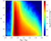 |
Fig. 4. Smoothed apparent Hess diagram of the conic sample constructed with the de-reddened Gaia DR2 colours and apparent magnitudes. |
2.1.6. Summary of the selection
We summarise the whole procedure of the Gaia samples selection as follows:
-
Firstly, we pre-select4 all stars in the truncated local 600 pc sphere with apparent magnitudes of 7 mag < G < 17 mag and within the colour range 0 mag < GBP − GRP < (3 + ϵ) mag (Sect. 2.1.4). The TAP queries used for this step are given in Appendix A. Then we apply more specific distance and colour-magnitude cuts: dmin < d < dmax, MG, min < MG < MG, max, and (GBP − GRP)min < GBP − GRP < (GBP − GRP)max + ϵ. This pre-selects different local populations as defined in Table 1. The colour range is extended towards the red part by ϵ = 0.5 mag in order to include stars that are reddened being located behind the nearby molecular clouds. The conic sample is pre-selected similarly, but with constraint on latitudes rather than distances, |b|> 80°.
-
Secondly, for all samples, we calculate de-reddened colours and magnitudes, applying the combined 3D extinction map from Green et al. (2019) and Lallement et al. (2018).
-
Afterwards we apply the adopted colour-magnitude cuts (Table 1) to the derived de-reddened colours.
-
The data are further cleaned from stars with unreliable astrometric parameters and photometry by applying cuts from Eqs. (2) and (3); in the case of the conic sample, only Eq. (3) is used. The numbers of stars in the final samples are given in columns 𝒩3 and 𝒩2 in Table 1.
-
For all samples defined on the absolute CMD we further select kinematic subsamples with known 6D phase space information and calculate the W-velocity component and its error for each star. The kinematic subsamples constitute ∼10% of the full colour-magnitude samples and the corresponding numbers of stars are listed in column 𝒩6 of Table 1.
-
Finally, we estimate the incompleteness introduced to each sample by our quality cuts and, in the case of kinematic subsamples, by the removal of stars without radial velocities. By comparing the number of stars in the final samples and in the samples before the radial velocity and/or quality cut were applied, we define a selection function 𝒮i given by Eqs. (4) and (5). The correction factor 1/𝒮i(l, b) is used as a weight for each star in the sample during the calculation of the quantities of interest.
2.2. APOGEE Red Clump sample
In addition to the Gaia data, we use the fourteenth data release (DR14) of the kinematically unbiased APOGEE RC catalogue, its earlier version was presented and discussed in Bovy et al. (2014). As the quality of the spectroscopic data is intrinsically high, we chose not to use any additional cuts with respect to the signal-to-noise ratio (S/N): its lowest value in the catalogue is 20, but only 2% of the stars have S/N < 50.
We split 29 502 APOGEE RC stars into the low- and high-α populations, which we later associate with the modelled thin and thick disk, respectively. To separate the populations, we use [Fe/H] and [α/Fe] provided in the APOGEE RC catalogue and define the boundary between the two populations in the following way (Fig. 5):
![$$ \begin{aligned} \mathrm [\alpha /Fe] = {\left\{ \begin{array}{ll} \ 0.07,&\mathrm{[Fe/H]} > 0 \\ \ -0.16 \mathrm{[Fe/H]} + 0.07,&-0.69 < \mathrm{[Fe/H]} < 0 \\ \ 0.18,&\mathrm{[Fe/H]} < -0.69. \end{array}\right.} \end{aligned} $$](/articles/aa/full_html/2021/03/aa38840-20/aa38840-20-eq6.gif)
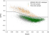 |
Fig. 5. Local low-α thin-disk (green) and high-α thick-disk (orange) samples selected for the analysis. The full APOGEE RC sample is shown in grey. The dashed black line marks the adopted boundary between the two populations, as in Eq. (6). |
As RC stars are bright giants with only a small scatter in luminosity, their spectrophotometric distances are very precise, the relative distance errors in the catalogue are ∼5% only. We convert these distances to Galactocentric cylindrical coordinates with the same values of (R⊙, z⊙) as in Sect. 2.1.2. Then we select stars in the range of Galactocentric distances R⊙ − ΔR < R < R⊙ + ΔR with ΔR = 0.5 kpc. In the case of APOGEE, we could not keep the sample extremely local as we did with Gaia by setting ΔR = 150 pc: there are only ∼2000 APOGEE RC stars located in such a narrow Solar annulus and this low number of stars is not enough for a reliable analysis. We further select low-α stars at distances from the Galactic plane |z|< 1 kpc, and high-α stars at |z|< 2 kpc.
To define the RC sample in the model, we use cuts on the synthetic effective temperatures Teff, log g, and luminosities L, Eqs. (18) and (19). Therefore, for the sake of consistency, we also apply the same cut on the effective temperature to the APOGEE data, selecting stars with 4250 K < Teff < 5250 K (the adopted cuts on log g and L mimic the selection criteria applied during the construction of the RC catalogue, so they do not need to be applied to the data). The final local low-α and high-α samples contain 3910 and 847 stars, respectively (Fig. 5).
In order to derive the AMR, we aim to reproduce the APOGEE RC metallicity distribution functions (MDFs) within our model framework (Sect. 4.5). As we do not try to predict the actual RC star counts but work only with the normalised MDFs, we are not interested in completeness of the selected APOGEE RC samples and do not include it into our analysis.
We also note, that though the individual precision of metallicity obtained by the APOGEE Stellar Parameter and Chemical Abundances Pipeline, ASPCAP, is very high, 0.01−0.02 dex, the overall uncertainty, including systematic errors may be as high as 0.1 dex (Jofré et al. 2019). This will inevitably add to the final uncertainty budget of the derived AMR.
3. JJ model update
The most recent version of the JJ model describes the Galactic thin disk as a set of isothermal mono-age stellar populations, whose evolution is governed by the four input functions: a declining SFR with a peak at old ages, a four-slope broken power-law IMF, and an AVR and AMR monotonously increasing with age (Sysoliatina et al. 2018a). A detailed description of the model was presented in Paper I, and the model machinery generalised for the whole Galactic disk will be summarised in an upcoming work (Sysoliatina and Just, in prep.). In this study we only concentrate on the new or updated model components.
3.1. Thin and thick disk
In this section, we explain our motivation for introducing a new treatment of the thick disk component: instead of a single mono-age subpopulation, we opt to use a set of subpopulations that represent a thick-disk SFR extended in time. As a result, we also have to update an analytic form of the thin-disk SFR function, such that the updated JJ model is able to reproduce our old results.
It is generally recognised that the high-α metal-poor population observed in our Galaxy mostly consists of old stars formed on a short time scale and constitutes a thick-disk component. In comparison to the low-α thin disk, it is more extended perpendicularly to the Galactic plane, less extended radially, and more dynamically heated. In Paper I, the thick disk was modelled in a simple way as a single-age isothermal component, that is equivalent to an assumption that the thick disk was formed during a single SF burst event. Yet many Galactic models treat the thick disk formation as a process extended in time, with a corresponding time scale ranging from as short as 0.1 Gyr (two-infall chemical models from Grisoni et al. 2018) to 4−5 Gyr as assumed in Haywood et al. (2013). It is not easy to probe the thick-disk age distribution with observational data, as stellar age determination is known to be very challenging and stellar ages obtained with different techniques have large uncertainties and may suffer from significant systematic errors. Nevertheless, available age maps provide a useful insight into the real age distribution in the Galaxy. Age maps constructed with the supervised classification method known as The Cannon (Ness et al. 2015), indicate that the age dispersion of the high-α APOGEE RC population may reach ∼1−2 Gyr, although individual age uncertainties were as high as ∼40% in this analysis. A more recent study on isochrone ages implies ∼1 Gyr age dispersion for the same stars, with individual age uncertainties reduced to ∼20% (Sanders & Das 2018). Therefore, we now allow a non-zero age spread for the thick disk in our model. To do so, we introduce the following thick-disk SFR as a function of Galactic time:

Here, sfrt(t) prescribes the shape of the SFR function: parameters γ and β control the SFR growth and steepness of its decline. The parameter tt15 determines the starting value of the SFR as  , and tp − tt2 is the maximum age of the thick-disk population with tp being the disk’s present-day age. The value of tp is set to 13 Gyr to be consistent with the typical age estimates derived for the oldest globular clusters in the Galactic bulge and halo (de la Fuente Marcos et al. 2015; Ortolani et al. 2019). With a time resolution of Δt = 25 Myr, this results in 160 isothermal subpopulations for the thick disk. The SFRt(t) function is normalised to the present-day thick-disk surface density Σt to describe the thick-disk formation history in physical units of M⊙ pc2 Gyr−1. An additional time-dependent function, gt(t), is necessary to account for the mass loss due to stellar evolution as not all of the mass converted into the thick-disk subpopulations at a given time, ti, survived to the present day in the form of stars or remnants. The mass loss function can be expressed as:
![$$ \begin{aligned} g(t) = 1 - \int _0^{t_\mathrm{p} } \int _{m(t)}^\infty \Delta m(\mathrm{[Fe/H]} (t),m) \frac{\mathrm{d}n}{\mathrm{d}m} \mathrm{d}m \ \mathrm{d}t .\end{aligned} $$](/articles/aa/full_html/2021/03/aa38840-20/aa38840-20-eq10.gif)
In this definition Δm([Fe/H](t),m) is a yield or total fraction of mass returned to the interstellar medium (ISM) in the form of processed material, which naturally depends on stellar mass and metallicity. The latter is prescribed by the model AMR function, [Fe/H](t). The differential ratio, dn/dm, corresponds to the model IMF and m(t) is a limiting stellar mass, such that only stars with masses larger than this limiting value contribute to the stellar feedback at a given time. In practice, the evaluation of the mass loss function, given the IMF and the thick-disk AMR, is performed with the chemical evolution code Chempy6 (Rybizki et al. 2017), where yields of asymptotic giant branch (AGB) and sypernovae (SNe) Type II stars are taken from Karakas (2010) and Nomoto et al. (2013), the ISM enrichment due to SNe Type Ia explosions are described by yields and delay time distribution (DTD) from Maoz et al. (2010), and stellar lifetimes are adopted from Argast et al. (2000). The thick-disk SFR parameters fixed in this work are given in Table 2.
JJ model parameters fixed in this work.
In order to be consistent with the earlier versions of the JJ model, we also re-define the thin-disk SFR:
Parameters td2, ζ, and η are chosen such that the cumulative SFR of the total disk closely follows the same function predicted by the JJ model used in Sysoliatina et al. (2018a). With SFRt parameters given in Table 2, we find the most suitable (td2, ζ, η) = (7.8 Gyr, 0.8, 5.6). The maximum of this thin-disk SFR function can be calculated according to the formula:
Motivated by the model-to-data inconsistencies already observed in Sysoliatina et al. (2018a) (see also Sect. 5), we add two additional Gaussian peaks to the thin-disk SFR:
Here (τp1, dτp1) and (τp2, dτp2) are the mean ages and dispersions of the additional SFR peaks and peak parameters Σp1 and Σp2 are related to their real amplitudes through  .
.
3.2. Gas model
In our previous works on the local disk model, starting from Paper I to the most recent testing of the model against the TGAS-RAVE data in Sysoliatina et al. (2018a), the gas component was defined in full analogy to the thin disk: we used a set of 180 isothermal gas subpopulations whose vertical kinematics was given by a scaled thin-disk AVR. In this paper, we use an easier and more physically motivated gas model: we introduce a two-component ISM consisting of molecular and atomic gas, H2 and HI, with the prescribed surface densities from McKee et al. (2015) and scale heights from Nakanishi & Sofue (2016).
At the Solar circle, the ratio of gas-to-stellar disk surface densities is ∼0.3, therefore a robust model of the gas component is crucial for the modelling of the local gravitational potential. At the same time, it is not easy to determine the local gas density from observations. In the case of atomic gas observed with the 21 cm line, it is challenging for several reasons: (1) overall number of molecular clouds is low which makes it difficult to determine their spatial distribution; (2) special corrections for optical thickness and presence of He and heavier elements must be applied. For molecular gas, two additional problems arise: (3) H2 is not observed directly, but is traced via CO, and CO-to-H2 conversion factor introduces a considerable uncertainly; (4) some fraction of molecular hydrogen can be ‘dark’ due to lower local concentration of CO as a tracer element. Additionally, the vertical fall-off of different gas components is usually assumed to be Gaussian and this simplification adds to the total uncertainty of the local gas density estimates.
For the local surface density of the molecular gas, we adopt 1.7 M⊙ pc−2 from McKee et al. (2015), which is the value from Flynn et al. (2006) updated with the new CO-to-H2 ratio recommended by Bolatto et al. (2013). This is the surface density for the Solar circle, and McKee et al. (2015) recommends the use of a lower density of 1.0 ± 0.3 M⊙ pc−2 for the Solar neighbourhood as the Sun is located in the Local Bubble. However, we do not apply this correction as we aim to apply our model to extended data samples. For the atomic gas we use 10.86 M⊙ pc−2 which is a sum of surface densities of the cold and warm atomic gas components from McKee et al. (2015). Our total gas surface density sums up to 12.86 ± 1.42 M⊙ pc−2. The vertical velocity dispersions of H2 and HI are then adjusted in our model to reproduce the observed thickness of the gas from Nakanishi & Sofue (2016) (Table 2).
Finally, we link the vertical kinematics of molecular gas to the vertical kinematics of the zero-age thin-disk subpopulation, as the latter is expected to inherit the vertical velocity dispersion of the material it was formed from. As before, the AVR is given as a power law, and is most conveniently defined in terms of age (Eq. (30) in Paper I):
This link between the gas and thin-disk vertical kinematics reduces the number of the model’s free parameters as it sets a constraint on one of the AVR parameters:
3.3. Stellar halo
In Paper II, a flattened spherical halo was used to fit the SDSS star counts towards the northern Galactic pole. In this study we treat the stellar halo as a single isothermal component of the age of 13 Gyr characterised by the vertical velocity dispersion of 100 km s−1 and the local surface density that is allowed to be optimised. At |z|≤2 kpc, where the Poisson-Boltzmann equation is solved, the vertical density profile of the halo is derived self-consistently with the total gravitational potential Φ(|z|). However, to simulate our conic Gaia sample, we need to assume the vertical density profile of the stellar halo at higher distances from the Galactic plane, |z|> 2 kpc. For this purpose, we adopt a broken power law. We define a radial Galactocentric coordinate,  , where q is a flattening parameter. As in practice our modelling is performed in the Cartesian grid, we write the halo density profile as a function of distance from the Galactic plane |z|. A breaking height that sets a boundary between the inner and outer halo is related to a breaking radius as
  , the value of rbr = 25 kpc is adopted from Bland-Hawthorn & Gerhard (2016). Then the general form of the halo vertical profile can be written as
Here (qin, αin) and (qout, αout) are flattening and slope of the inner and outer halo, respectively. Their values taken from Bland-Hawthorn & Gerhard (2016) are listed in Table 2. The scaling parameters,  and
and  , are chosen such that they ensure continuity of the profile at |z| = 2 kpc and |z|=zbr. Division by R⊙ is added as the scaling densities are given for the Solar position.
4. Method
With the specified input functions {SFR, IMF, AVR, AMR}, as well as several additional model parameters (Table 2), the Poisson-Boltzmann equation is solved iteratively. This returns a self-consistent pair of the gravitational potential and the vertical density law, {Φ(|z|), ρ(|z|)}. Then the derived density profiles of the thin- and thick-disk and halo mono-age subpopulations are used to model the local samples with different photometric properties. Using a stellar evolution library, we locate our mono-age subpopulations in the 3D age-metallicity-mass space (Sect. 4.1). Finally, with photometric information added from the isochrones, we are able to reproduce the spatial distribution of samples selected on the CMD, as well as model different selection effects (Sects. 4.2–4.5).
4.1. Stellar population synthesis
We follow the scheme described in our previous study (Sysoliatina et al. 2018a). For the sake of completeness, we summarise the main points of this procedure here.
We populate the 3D age-metallicity-mass parameter space using age-metallicity pairs prescribed by the adopted AMR and stellar masses given in isochrones. Following Sysoliatina et al. (2018a), we use the term ‘stellar assembly’ to refer to a set of stars characterised by the same age, metallicity, and mass. We take a set of 62 isochrone tables generated with the PAdova and TRieste Stellar Evolution Code (PARSEC v.1.2S; Bressan et al. 2012) and the COLIBRI code (v. S_35; Marigo et al. 2017) for the thermally pulsing asymptotic giant branch (TP-AGB) phase7. The selected isochrones cover a wide metallicity range, [Fe/H] = −2.6…+0.47, and are generated with a linear age step of Δτ = 50 Myr. The total number of stellar assemblies of the thin disk, thick disk, and halo sum up to ∼6.6 × 10⁵. Each of our mono-age isothermal subpopulations of the disk is characterised by metallicity drawn from the AMR function (Sect. 4.5). In the case of the halo we use a set of metallicities drawn from the Gaussian metallicity distribution (Sect. 4.3). Then, for a given age-metallicity pair we chose an isochrone with the closest age and metallicity values. Finally, each of the age-metallicity-mass stellar assemblies from the chosen isochrone is further assigned with a surface number density prescribed by the SFR and IMF.
In order to check the impact of the stellar library on our results, we also use an alternative set of isochrones from MESA (Modules and Experiments in Stellar Astrophysics, Paxton et al. 2011, 2013, 2015) Isochrones and Stellar Tracks (MIST8, v.1.2; Dotter 2016; Choi et al. 2016) (see Sects. 5.3.3 and 6.1.3). The MIST isochrones are used with the same metallicity and age grid as the isochrones generated by PARSEC.
4.2. Vertical profiles and velocity distributions
To simulate the samples of A, F, and RC stars and G, G/K, and K dwarfs, we apply colour-magnitude cuts from Table 1 to the set of stellar assemblies, fully analogously to criteria applied to the data. Here we use synthetic Gaia passbands from Maíz Apellániz & Weiler (2018).
At this point, the construction of the number density profiles and velocity distribution functions of the mock samples is quite straightforward. The number density profiles are calculated according to Eq. (4) from Sysoliatina et al. (2018a) with |z|-resolution of 20 pc. The velocity distribution functions f(|W|) are derived as a sum of Gaussian distributions with known dispersion weighted by the number of stars in a given volume. Here the W-velocity dispersions of the thin-disk populations is prescribed by the AVR, Eq. (13), and parameters σp1 and σp2 that are associated with the recent periods of the SF enhancement (more in Sect. 4.6.2). The thick-disk and halo velocity dispersions, σt and σsh, are listed in Table 2. We trace the f(|W|) shape up to |W|max = 60 km s−1 and set the velocity resolution to Δ|W| = 2 km s−1 as this bin size is larger than a typical velocity error in the bin which is ∼0.7 km s−1.
4.3. Conic sample modelling
In order to model our third quantity of interest, the Hess diagram of the conic sample, we need to make several additional steps.
As explained in Sect. 4.5, we use APOGEE RC stars to constrain the AMR functions of the thin and thick disk. In the case of the stellar halo, we assume a Gaussian metallicity distribution with mean metallicity and dispersion (⟨[Fe/H]⟩,σ[Fe/H]) = (−1.5, 0.4). From this distribution, we draw nine metallicity values and use them in combination with halo age of 13 Gyr to select isochrones. The total number density assigned to the halo stellar assemblies is normalised to its present-day surface density up to |z| = 2 kpc.
In order to optimise computation time needed to produce the mock Hess diagram of the conic sample, we use a grid with a variable |z|-step. To define such a grid, we use the condition
where ΔG = 0.1 mag is the apparent magnitude resolution of the Hess diagram. Close to the Galactic plane, we also check that the vertical resolution of our grid is not better than 2 kpc, as this is the vertical resolution, Δz, adopted for the reconstruction of the vertical gravitational potential (see Table 2). Defined by Eq. (16), the vertical step of such a grid grows linearly with |z|, and reaches ∼6 kpc at height |z| = 130 kpc that is a height up to which we model the halo profile.
We also ignore the vertical offset of the Sun and assume that it is located exactly in the Galactic plane. In the case when z⊙ = 20 pc is taken into account, the summation of the stellar densities in the directions to the northern and southern Galactic poles must be performed separately up to ∼0.9 kpc (further away from the Galactic plane south-north differences in the apparent magnitudes of stellar assemblies become smaller than the adopted resolution ΔG). This results in smoothing of the Hess diagram along the vertical axis, apparent magnitude G, although all the features change only slightly. At the same time, Hess diagram computation time almost doubles, which may have a great impact on the final calculation time of our MCMC sampling (Sect. 5.1). As we smooth the mock Hess diagram later, the effect of z⊙ is essentially masked and, therefore, we decided to ignore the Solar offset in this case. We note, however, that this is done only for the conic sample and in the case of the number density profiles and vertical velocity distributions, z⊙, value from Table 2 is properly taken into account during the selection of the stellar assemblies representing the Gaia samples.
As the self-consistent density-potential pair {ρ(|z|), Φ(|z|)} is calculated within the model up to 2 kpc only (see parameter zmax in Table 2), we need to extrapolate the derived density profiles to larger heights in order to model all stars within the conic volume. The thin disk is a plane-concentrated component, therefore we model its populations up to 2 kpc only. To include the thick disk, we fit its vertical profile with a sechαt law of a single isothermal population. As in Paper II, we find that the vertical profile of the thick-disk component follows the sechαt law very closely as it is kinematically homogeneous. So we use such an extrapolation to model the thick-disk stellar assemblies up to 12 kpc from the Galactic plane. The vertical profile of the halo is chosen to be a broken power law and is given by Eq. (15). Although the opening angle of the cone is relatively small, θ = 20°, at large heights above the Galactic plane the conic sample is not local any more. Therefore, at each |z| we take a mean halo density in this horizontal slice. Also, at each |z| stellar assemblies of all components are exposed to the same cut on apparent G-magnitudes as was applied to the data, 12 mag < G < 17 mag (Table 1).
4.4. Model optimisation procedure
Before explaining how we constrain the AMR function, we outline the overall scheme of the model optimisation carried out in this work.
Once they have been constructed for the initial input functions {SFR, IMF, AVR, AMR}0, stellar assemblies can be used to simulate model predictions with the modified SFR and IMF. This is possible because changes in shapes of these functions can be taken into account simply by adding corresponding weights sensitive to stellar ages and masses. However, a modification of the AMR function implies that for each modelled mono-age population a new isochrone has to be chosen, and the whole process of weighting the SFR with IMF functions has to be repeated for the new stellar assemblies. As this process is relatively time-consuming, it is not possible to update the AMR on-the-fly as only a short model-to-data comparison time is acceptable for an exploration of the multidimensional parameter space with the MCMC method. Among the four model input functions, including the AVR (which implicitly prescribes how the populations are distributed perpendicular to the Galactic plane), the weakest impact on the predicted self-consistent density-potential pair is from the AMR function. Taking this into account, we developed the following model optimisation scheme:
Firstly, we constrain the chemical evolution history given initial {SFR, IMF, AVR}0. To do so, we simulate the local RC sample (Sect. 2.2), and iteratively converge to AMR0 such that the observed metallicity distributions of the high- and low-α APOGEE RC stars are best reproduced within this model (Sect. 4.5).
Secondly, we use the MCMC technique to adapt the most important model parameters self-consistently (Sect. 4.6). At this step, the shape of the AMR0 function is not varied.
Finally, using the new functions {SFR, IMF, AVR}′ obtained in the previous step, we update the chemical evolution part of the model following the strategy from step (1). This sequence of steps is repeated until the process converges to a fully self-consistent set of the model functions {SFR, IMF, AVR, AMR}′. In practice, we find that all changes to the model parameters become negligible as soon as just after the second iteration.
4.5. Age-metallicity relation with APOGEE RC
In order to constrain the AMR function, we perform a direct comparison between the observed metallicity distribution of the high- and low-α APOGEE RC stars (Sect. 2.2) and the predicted age distributions of the thin- and thick-disk RC populations in the model.
The left panel of Fig. 6 shows the cumulative metallicity distribution functions (CMDFs) calculated for two selected RC samples and smoothed with the Savitzky-Golay filter (grey crosses). A highly non-linear behaviour of the observed CMDFs in the low- and high-metallicity regimes can be associated with metallicity uncertainties or systematic errors. Otherwise, under the assumption that the low and high metallicity values correspond directly to the old and young stellar ages, this picture implies a very rapid enrichment in the beginning of the Galactic evolution and during the last ∼1−2 Gyr of both thin- and thick-disk formation. The first of these epochs of fast ISM enrichment is naturally associated with an early phase of the Galactic evolution characterised by intense SF processes. However, a recent rise of the ISM enrichment rate, as implied by the low-α CMDF, contradicts a variant of the mediocrity principle that assumes that the time we live in is not special. Alternatively, the most metal-rich stars in both samples may be stars that migrated to the Solar radius from the inner Galaxy, thus, they are not necessarily the youngest populations in the samples. Within the naive approach applied here, we do not aim to distinguish between the two above-mentioned interpretations of the non-linear, metal-rich parts of the observed CMDFs. We rather aim to reconstruct the AMR that: (1) predicts a monotonous increase of metallicity with Galactic time; and (2) does not demonstrate any special behaviour in the end of both thin- and thick-disk evolution phases. The residual deviations from such AMR functions are included in the form of an error model.
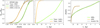 |
Fig. 6. AMR reconstruction. All model predictions shown here are generated with the best-fit parameters of MCMC1 model (Sect. 5). Left: normalised CMDFs of the high- and low-α APOGEE RC samples. Grey crosses show the smoothed data, thick black lines are the ‘deconvolved’ CMDFs (see text), and the full coloured lines illustrate the result of the convolution of the ‘deconvolved’ CMDF with Gaussian kernels. Middle: modelled CADFs for the thin and thick disk RC populations. Right: resulting AMR for the thin and thick disk. Analytic fits are over-plotted with black dashed curves. |
We assume that the shape of the metal-rich parts of both observed CMDFs can be expressed as a result of the convolution of a linear function with a Gaussian kernel. Here, the former corresponds to observations fully consistent with our AMR of interest and the latter represents the effect of observational errors or the presence of migrated stars. Analytically, this convolution C(x) can be expressed as:
![$$ \begin{aligned} C(x)&= \frac{1}{2}(kx+b) \cdot \left[\mathrm{Erf} \left(\frac{kx+b}{\sqrt{2}k\sigma } \right) - \mathrm{Erf} \left(\frac{kx+b-1}{\sqrt{2}k\sigma } \right) \right] \nonumber \\&\quad + \frac{k\sigma }{\sqrt{2\pi }}\left[\exp {\left(-\frac{(kx+b)^2}{2k^2\sigma ^2}\right)} - \exp {\left(\frac{(kx+b-1)^2}{2k^2\sigma ^2}\right)}\right] \nonumber \\&\quad + \frac{1}{2}\left[1 + \mathrm{Erf} \left(\frac{kx+b-1}{\sqrt{2}k\sigma }\right)\right], \quad \text{where} \quad x=\mathrm{[Fe/H].} \end{aligned} $$](/articles/aa/full_html/2021/03/aa38840-20/aa38840-20-eq23.gif)
Here, k and b are slope and offset of the CMDF linear part, and σ is a the Gaussian dispersion. We use Eq. (17) to fit the upper parts of the observed CMDFs of the high- and low-α APOGEE RC samples, Ncum/Ntot > 0.5. We use their full linear parts Ncum/Ntot = 0.3...0.7 to calculate parameters k and b. Then values of σ needed to reproduce the metal-rich tails of CMDFs are found to be ∼0.1 dex and ∼0.13 dex for the thin and thick disk, respectively. The ‘deconvolved’ linear trends of the metal-rich parts of the observed CMDFs are shown with black thick lines in Fig. 6. These ‘deconvolved’ CMDFs are later used for the AMR reconstruction.
In order to proceed, we assume that there is a unique correspondence between metallicities in the ‘deconvolved’ CMDFs and stellar ages in the Solar neighbourhood. This is known to be a simplification, but in Sect. 6.1.5, we argue that this approach is nevertheless reasonable enough for our analysis. We synthesise the stellar assemblies that represent thin and thick disk as explained above. To do so, we specify the model functions {SFR, IMF, AVR}0, and assume initial functions AMRini. From the generated stellar assemblies, we select RC stars by applying the following cuts:

![$$ \begin{aligned} \log {g}&< \mathrm{min}(2.9, 22.5 \log {T_\mathrm{eff} } - 80.1 + 0.5 \mathrm{[Fe/H]} ). \end{aligned} $$](/articles/aa/full_html/2021/03/aa38840-20/aa38840-20-eq25.gif)
Here, Eq. (18) selects stars in the temperature and luminosity range corresponding to the location of RC at the Herzsprung-Russel diagram (HRD). The general form of the second cut given by Eq. (19) is taken from the analysis of the APOGEE giants performed in Bovy et al. (2014), where the authors used a similar criterium to clean the RC sample from the red giant branch (RGB; see their Eqs. (2) and (3)). The exact coefficients of Eq. (19) are different to those given in Bovy et al. (2014), as the authors used an older version of Padova isochrones, so their selection cannot properly separate RC and RGB stars in the {log g, log Teff, [Fe/H]} parameter space of the updated stellar library used in this work. We also find that Eq. (19) is not useful when the MIST isochrones are used and it needs to be modified also in this case. For the sake of completeness, we also show our second version of Eq. (19), which can be used together with the MESA stellar evolution library:
![$$ \begin{aligned} \log {g} < \mathrm{min}(2.9, 22.1 \log {T_\mathrm{eff} } - 78.4 + 0.6 \mathrm{[Fe/H]} ) .\end{aligned} $$](/articles/aa/full_html/2021/03/aa38840-20/aa38840-20-eq26.gif)
Using our mock RC stellar assemblies and modelled vertical gravitational potential, we predict the vertical number density profiles of the RC stars up to the heights of |z| = 1 kpc and |z| = 2 kpc for the thin and thick disk, respectively (by analogy to the data selection criteria in Sect. 2.2). The cumulative age distribution functions (CADFs) calculated for these mock RC samples are shown in the middle panel of Fig. 6.
Finally, each metallicity from the ‘deconvolved’ CMDF is assigned with an age from the corresponding modelled CADF. The resulting AMR usually differs from the initial function AMRini, unless the initial guess is very good. To bring the derived AMR into the full consistency with the assumed {SFR, IMF, AVR}0, the generation of the RC age distributions is repeated three to four times. During each iteration, we use the AMR derived in the previous cycle to update our stellar assemblies, as well as the mass loss function. In the end, the procedure converges to our target AMR0.
For convenience, we also fit the thin- and thick-disk AMR functions with the following equation:
![$$ \begin{aligned} \mathrm{[Fe/H]} (t) = \mathrm{[Fe/H]} _0 + (\mathrm{[Fe/H]} _\mathrm{p} -\mathrm{[Fe/H]} _0) \cdot f(t), \end{aligned} $$](/articles/aa/full_html/2021/03/aa38840-20/aa38840-20-eq27.gif)
where [Fe/H]0 and [Fe/H]p are the initial and present-day metallicity values and
The CADFs, as well as the thin-disk and thick-disk AMR functions shown in the right panel of Fig. 6, are consistent with the updated parameters of the JJ model presented below in Table 4 (MCMC1 model). The best-fit parameters of Eqs. (21) and (22) are summarised in Table 3.
4.6. Bayesian analysis
In order to improve the JJ model parameters, we use Bayes theorem. It links posterior ℙ(m|d) expressing a probability of a model based on the given data, the likelihood ℒ(d|m) describing a probability to observe some data based on a given model, and prior 𝒫(m) expressing our initial knowledge about the model parameters:

It is common to write Eq. (23) in logarithmic scale with likelihood and posterior normalised to their maximum values:
In the subsections below, we explain how the likelihood and prior are calculated and we specify a set of model parameters chosen for optimisation.
4.6.1. Likelihood
The likelihood function is aimed at describing a model-to-data goodness of fit in terms of the three different types of data: vertical number density profiles, W-velocity distribution functions, and apparent Hess diagram of the conic sample. As there is no standard recipe for how to combine probabilities from different data types, we use the following method: each data type is set to correspond to a separate term in the logarithmic likelihood and separately normalised on its own value that is calculated for a set of parameters we refer to as ‘standard’ (Sect. 4.6.2). This approach ensures that the contributions of these three terms to the total likelihood are comparable, such that all data types have similar weights during the fitting procedure.
To make the final formula for the likelihood more compact, we introduce several definitions. We have the indices (z, W, H) corresponding to the type of quantity a given term refers to: vertical profiles, kinematics, and Hess diagram, respectively. Superscripts (m, d) mark model or data origin of some value. We also define the number of |z|- and |W|-bins used to calculate the vertical number density profiles and velocity distributions from the selected Gaia samples as Bz and BW, respectively. Then BW is the same for all samples with known vertical kinematics, BW = |W|max/Δ|W| = 30, and Bz depends on the vertical extent of the sample and may vary. In the case of the apparent Hess diagram of the conic sample, BH is the total number of colour-magnitude bins given by the adopted colour-magnitude resolution (Sect. 2.1.5): BH = 60 × 50 = 3 × 10³. The number of samples used to fit star counts and kinematics are denoted as Sz = 6 and SW = 5, respectively (Table 1). Finally, notations nz and nW correspond to the number density of stars per |z|- or |W|-bin, and NH is the actual number of stars in a colour-magnitude bin at the Hess diagram.
In terms of these definitions, and with θ0 being the vector of standard parameter values, the general expression for the normalised logarithmic likelihood is written as:
The first term in Eq. (25) quantifies consistency between the number density profiles derived from our selected Gaia samples and the number density profiles predicted by the JJ model for the same stellar populations:
This formula returns a mean of the relative deviation between the predicted and observed number density per |z|-bin (expression in brackets), which is also averaged over all samples. As the actual number density values may vary by several orders of magnitude within the studied volume (see Fig. 9), it is more sensible to measure the relative model-to-data deviations in logarithmic scale. In this case, the fitting procedure is sensitive to both the cores and tails of the density profiles.
The second likelihood term in Eq. (25) gives a measure of the consistency between the observed and predicted |W|-velocity distributions. We define it in a way similar to Eq. (26), but using a linear scale for model-to-data relative deviations per velocity bin:
The observed and synthetic apparent Hess diagrams are compared in terms of χ2 translated into a logarithmic space (Paper II):
By analogy to Eqs. (26) and (27), this formula returns a logarithmic χ2 per colour-magnitude bin averaged over the whole apparent Hess diagram.
As we prefer to divide the absolute model-to-data differences by a smooth function, all model-to-data deviations in Eqs. (26)–(28) are calculated relative to the model predictions, that are free of noise.
4.6.2. Prior
We define our logarithmic prior as a sum over Gaussian probabilities:
where ⟨θ⟩i and Δθi are the mean and dispersion of parameter θi, and the sum is taken over θ, the full vector of parameters chosen for optimisation.
While specifying the vector θ, we tried to include all key parameters that influence predicted star counts and kinematics. Several new parameters were introduced in order to achieve an adequate consistency between the model and data. At the same time, we tried to keep the number of free parameters minimal, as an increase of the parameter space dimension leads to a non-linear increase of the computation time needed to find the best model. With these considerations taken into account, we selected for the optimisation the following model parameters (see Table 4 for a summary):
JJ model parameters optimised in this study.
The first four of these parameters refer to the surface densities of the thin and thick disk, the DM, and the stellar halo. These parameters play a role of the local normalisation of the model components’ vertical profiles. Here, Σd and Σt strongly influence the total predicted number of stars, while the DM surface density Σdh impacts the shape of the vertical gravitational potential and, thus, affects the vertical fall-off of all populations. The parameter Σsh has very moderate impact on the vertical profiles and kinematics, but is important for the reconstruction of the conic sample, whose significant fraction constitutes of halo stars. The mean prior values of the surface densities of the thin and thick disk are taken close to the values from the original JJ model (Paper I, Table 2) and allow for reasonably large dispersions ⟨θ⟩i. The mean value of the surface density of the stellar halo is adopted from Flynn et al. (2006).
In the case of the DM surface density, its expectation value is set to 50 M⊙ pc−2, which is ∼17% lower than the best value from Paper I, where Σdh = 59.9 M⊙ pc−2. This change is motivated by recent results in measurements of the local DM density, ρdh. The values of ρdh estimated from the Galactic rotation curve usually lie in the range of 0.005−0.015 M⊙ pc−3 (Read 2014); similar measurements obtained from the Gaia DR2 rotation curve suggest an even narrower range, namely, ∼0.3−0.4 GeV cm−3 (∼0.008−0.011 M⊙ pc−3) (de Salas et al. 2019). Assuming a roughly constant DM density up to 2.3 kpc away from the Galactic plane at the Solar radius (as our old value of Σdh corresponds to |z|< 2.3 kpc), this translates to Σdh ≈ 23−69 M⊙ pc−2 or, with more conservative constraint from de Salas et al. (2019), to Σdh ≈ 37−51 M⊙ pc−2. Our old value lays at the high end of the range, and therefore is not optimal for the prior mean. With the assumed mean value of 50 M⊙ pc−2, we still favour the heavy DM halo. However, the fitting procedure is allowed to extend the investigation to much lower values, as we set a large dispersion of 10 M⊙ pc−2.
The second row of Eq. (30) lists the kinematic parameters explored in this study. The first two of them, σe and α, are the scale parameter and the slope of the AVR function, Eq. (13). These parameters have a direct impact on the vertical gravitational potential through the thin-disk kinematics. They are also known to be correlated, but we chose to constrain both σe and α, as it is hard to determine a priori the strength of the correlation and whether using only one of them will result in the same model flexibility. We also aim to constrain the vertical velocity dispersion of the thick disk given by σt. Parameters σp1 and σp2 prescribe the vertical velocity dispersion of the thin-disk stellar populations related to the additional peaks in the thin-disk SFR function, Eq. (12). These are new model parameters that have been introduced to reduce the observed discrepancies between the Gaia data and the JJ model predictions, mainly in terms of the vertical number density profiles of the young stellar populations (Sect. 5.3.1). Their prior means ⟨σp1⟩ and ⟨σp2⟩ represent our initial guess motivated by a simple test (Sect. 5.3.1) and the corresponding dispersions are chosen such that an exploration of a reasonably wide range of velocity values is permitted.
The third row of Eq. (30) contains parameters that govern the shape of the thin-disk SFR. By changing the combination of slopes (ζ, η), both the amplitude and position of the SFR peak at old ages can be changed, as well as the steepness of the SFR decline. The next six parameters describe the amplitude, position, and duration of the two recent peaks of the thin-disk SFR that are tested in this work.
The first of the new peaks corresponds to the recent SF burst found by Mor et al. (2019). From this work we adopt the mean age and mean dispersion of the peak, τp1 = 3 Gyr and dτp1 = 0.7 Gyr, respectively. The second of the additional SFR peaks is set to the most recent past of τp2 = 0.5 Gyr ago with a width of dτp2 = 0.25 Gyr. This choice is motivated by the observed shape of the vertical number density profile of the young A stars that indicates a presence of a dynamically hot and extremely young population (Sect. 5.3.1). The adopted dispersion for τp2 is set to be large, also 0.5 Gyr, such that mean age of the second SF burst can formally turn negative (i.e., in the future). This is done in order to test the possibility of the SF enhancement happening in the present day. As for the amplitudes of these additional SFR peaks, we set their mean values to zero, which implies that initially we do not assume any recent SF bursts in the disk formation history. However, wide priors of these parameters allow for the fitting procedure to put them into play in case their presence improves the model-to-data consistency.
Finally, the last five parameters of the vector θ refer to the slopes of our broken power-law IMF and positions of the breaks between the slopes {α0 and α1} and {α1 and α2}. We find it necessary to investigate the IMF shape self-consistently with the SFR shape normalisation as both SFR and IMF influence the present-day age distributions and star counts. We do not explore the fourth IMF slope α2 corresponding to the high-mass regime m > 6 M⊙ as stars of these masses are essentially absent in our data samples as they are too bright for the applied apparent magnitude cuts. The mean values of these parameters are chosen close to the IMF parameters from Paper III (also Rybizki 2018), and the adopted dispersions ensure reasonably wide priors.
As already mentioned in Sect. 4.6.1, we also define a set of standard values of model parameters θ0. These standard values are either directly taken from the previous works (Paper I-Paper III) or, in cases where the description of a model component was modified, they are chosen such that our previous results are closely mimicked. The set of standard parameters is also given in Table 4.
5. Results
5.1. Setup of MCMC runs
We use the Python realisation of the affine-invariant ensemble sampler for MCMC: the emcee module (Foreman-Mackey et al. 2013). This code is efficiently parallelised that allows us to perform calculations on multiple CPU cores. The number of cores that can be used by emcee is related to the number of walkers as ncore = nwalker/2, and the number of walkers must be at least twice the number of parameters, nwalker ≥ 2nparam. In our case, nparam = 22, so we set nwalker = 44. There are several ways to initialise walkers, one of them is to set parameter values very close to their means, that is, to distribute them in a small cloud around ⟨θ⟩. Here, we use a different approach: each walker is initialised with a set of parameter values drawn randomly from the allowed intervals [⟨θ⟩−3Δθ, ⟨θ⟩+3Δθ]. As recommended in Foreman-Mackey et al. (2013), we check the procedure performance and convergence using the integrated autocorrelation time  . This value gives an idea of the number of steps required to achieve a representative posterior sampling. We set the maximum number of steps in the MCMC chains to nmax = 5 × 10⁴, and the convergence is usually achieved after (4.4−4.5) × 104 steps. We also check the mean value of the MCMC acceptance fraction, af, which is a fraction of the proposed steps accepted by the MCMC routine. For well-behaved chains, it should remain in the range of af = 0.2…0.5, which is fulfilled during the MCMC runs performed for this study. In order to select independent samples from our chains, we remove the first
  steps corresponding to a burn-in phase, and select every
  -th step from each chain. With the mean autocorrelation time being approximately
  for our simulations, we obtain ∼103 independent samples drawn from the posterior probability distribution function (PDF) that we are interested in.
5.2. Three models
In this section, we describe and discuss three realisations of the JJ model which are presented in Table 4. The first model relies on the standard parameter values θ0 and is referred to as the standard model. In order to investigate the model parameter space, we perform two MCMC simulations, as explained in Sect. 5.1.
Our first run explores the posterior PDF using stellar assemblies synthesised with the PARSEC stellar library. The sampled posterior PDF projected onto different parameter axes and marginalised over the least interesting model parameters is shown in Fig. 7 (the full posterior PDF is presented in Fig. C.1). The four colours highlight different parameter groups discussed in Sect. 4.6.2. The colored histograms on the diagonal of Fig. 7 show the normalised PDFs for each parameter, Gaussian distributions plotted in black dashed lines correspond to the adopted prior and the light-blue histograms present the normalised likelihood PDFs. Thin grey lines mark θ0, and the most probable parameter values are shown with large black crosses. We note that the cross positions can be not perfectly aligned with the visible probability maxima at the 2D projections as the real multidimensional PDF can have a complex shape. The best parameters, along with their 16 and 84 percentiles determined within this MCMC simulation, constitute a new optimised model which we henceforth refer to as MCMC1 model (Table 4).
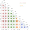 |
Fig. 7. Posterior PDF marginalised over the least important parameters from the set θ. The probability distribution is sampled during the MCMC1 simulation. Thin grey lines mark the standard values of parameters θ0 and black crosses show their new best values. Histograms on the plot diagonal show each parameter PDF (coloured steps), Gaussian priors (dashed black curves), and the likelihood PDFs (light-blue steps). |
Additionally, in order to test how the choice of stellar evolution library impacts our results, we perform a complementary run of the MCMC simulation. In this case, we sample posterior distribution using the mock stellar assemblies calculated with the MIST isochrones. The best parameter values of this test are also listed in Table 4 (MCMC2 model, hereafter).
We recall here that both of the described MCMC posterior samplings require an iteration (Sect. 4.4). At first, they are performed using stellar assemblies synthesised with some initial APOGEE-based AMR0. Afterwards, the AMR function is updated using the new optimised set of model parameters (Sect. 4.5) and the stellar assemblies are re-calculated. In the end, we run a closure MCMC simulation based on the new stellar assemblies set. The posterior PDF shown in Figs. 7 and C.1 and the derived MCMC1 and MCMC2 model parameters given in Table 4 are the result of such iteration, that is, they are self-consistent with the APOGEE-based AMR. The AMR functions of the MCMC1 and MCMC2 models are found to be essentially identical, so both of the models have an AMR shown in the right panel of Fig. 6.
5.2.1. New parameters and correlations
We analyse the derived multidimensional PDF shown in Figs. 7 and C.1 and the parameter values obtained from it of the MCMC1 model.
As we can immediately see from Table 4, almost half the investigated parameters have optimised values that are very close to the corresponding prior means. For a given parameter, this implies two possibilities: (1) our initial guess of prior was already very good, or (2) model predictions are not sensitive to this parameter, so it cannot be constrained within the current framework. We note, however, that this reasoning does not apply for correlated parameters; in this case, even the flat likelihood distribution does not necessarily mean that the quantity is entirely unconstrained (see below). Putting aside for a moment the question about correlations, we can distinguish between the two mentioned cases if we plot the normalised likelihood PDFs for each parameter (light-blue histograms in Figs. 7 and C.1). When the likelihood is sampled, our prior knowledge of the model parameters is ignored and the two above-mentioned possibilities can be distinguished. If the mean prior value is estimated well, then also the likelihood PDF demonstrates a peak around the prior maximum. On the other hand, if the model predictions are only weakly sensitive to some parameter or not sensitive at all, then the likelihood PDF projected onto its axis is expected to be approximately flat.
We find that we are not able to put reliable constraints on several parameters, including the width of both recent SF bursts controlled by dτp1 and dτp2, for which the MCMC routine returned the adopted prior means. The vertical velocity dispersion associated with the younger of the bursts, σp2, is constrained only weakly and from the likelihood PDF, we only see that the values σp2 > 12 km s−1 are preferred (Fig. C.1). In addition, the SFR parameter η does not appear to be important and varying the SFR parameter ξ alone is enough to improve the model performance.
We also see that in most cases, pairs of the selected parameters are uncorrelated, implying that they are essentially independent and, therefore, well chosen. However, if Figs. 7 and C.1 are thoughtfully inspected, the expected correlation between SFR and IMF can be noticed, as well as the (less strong) correlation between the SFR and thin- and thick-disk kinematics. This justifies our initial reasoning (Sect. 1) that in order to constrain the SFR in a robust way, its shape has to be adapted self-consistently not only with the IMF, but also with kinematic parameters. Also, a positive correlation is observed between the thin-disk kinematic parameters, σe and α, which we mention in Sect. 4.6.2. The surface density of the DM halo Σdh is correlated negatively with σe and the thick-disk velocity dispersion, σt, and positively with the IMF parameters, α1 and α2, forming an ambiguity that we cannot resolve here. Thus, although Σdh seems to be poorly constrained at first glance (flat likelihood PDF; most probable value very close to the assumed prior mean), it is not entirely unknown, as it is implicitly constrained via correlations with other parameters. Finally, the IMF parameters are found to be not entirely independent from each other, there are moderate correlations between pairs (α0, m0), (α1, m1), and (α0, α1).
5.2.2. Age distributions
Before presenting predictions of the optimised model MCMC1 and discussing them in detail, together with the reference standard model and test MCMC2 model, we show mock age distributions for the six Gaia samples selected on the CMD, as well as for the conic sample (Table 1). Figure 8 shows the normalised age distributions of the samples that correspond to the predictions of the MCMC1 and MCMC2 models (dashed and solid coloured lines, respectively). Grey histograms are the relative contributions from the halo (τ = 13 Gyr), thick disk (τ > 9 Gyr), and thin disk (all ages) to the overall age distributions of each sample. Figure 8 illustrates the differences in age coverage between the selected samples which we referred to as part of the sample selection in Sect. 2.1.1. We also see that the MIST isochrones are generated with a better interpolation scheme than the PARSEC isochrones, such that the age distributions corresponding to the MCMC2 model look much smoother.
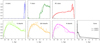 |
Fig. 8. Age distributions of the Gaia samples used for the optimisation of the model parameters θ. Dashed and solid coloured lines correspond to the predictions obtained with the set of MCMC1 and MCMC2 model parameters, respectively. Grey histograms show the relative contributions of the halo, thick-, and thin-disk components (τ = 13 Gyr, 13 Gyr > τ > 9 Gyr, and all ages, respectively). The samples are typically dominated by the thin-disk stars, e.g. the overall age distributions of A and F stars essentially coincide with the thin-disk contributions, as the thick disk and halo entirely or almost entirely miss in this case. The only sample with a considerable fraction of the thick-disk and halo (∼50%) consists of the stars selected towards the Galactic poles (lower-right panel, also see Fig. 11). |
5.3. Model predictions
5.3.1. The standard model and its weaknesses
For the purposes of illustration, it is handy to present a detailed description of the standard model performance, as some of the observed model-to-data discrepancies served as a motivation for us to introduce the new model features described in Sect. 3.
Figure 9 shows the vertical number density laws. The observed profiles calculated for the six Gaia samples (Table 1) are shown with black crosses. The coloured curves correspond to the three JJ model realisations, the standard model predictions are plotted in red. There is a number of discrepancies observed in this case. First, we see significant negative or positive offsets between the observed and predicted density profiles for all samples except A stars and K dwarfs. The predicted shape of the RC number density profile is fully realistic, but the actual number of RC stars in the volume is overestimated by ∼33%. We note that the number of stars in the data samples given in Figs. 9–11 do not exactly match the sample statistics summarised in the corresponding columns of Table 1. This happens because the quantities of interest are calculated from the data with the help of weights 1/𝒮i(l, b) that compensate for the small incompleteness effects introduced by our data selection and cleanings (Sect. 2.1.3). For K dwarfs, the predicted number of stars in the local volume matches the observed one within 1%, but this consistency arises from a lucky combination: the lack of K dwarfs close to the Galactic plane, at |z|≲100 pc, is compensated by the excess of modelled K dwarfs at larger distances, |z|≳200−250 pc. For the rest of the samples the observed number density profiles are not followed by the modelled ones as well. In general, profiles of the MS stars in the model are somewhat shallower than is suggested by the data, the overall number of stars in the G- and G/K- dwarf samples is overestimated by ∼20% and ∼15%, respectively. The predicted vertical profile of F stars is too steep, and the number of F stars in the volume is underestimated by ∼26%. The same ∼25% lack of stars is observed for A stars. The inner part of the number density profile of A stars, |z|< 300 pc, fits the observed profile well, however we see a significant discrepancy between the data and model further from the Galactic plane: the predicted number density falls off too steeply and is unable to reproduce the change in profile slope that happens at |z|≈300−350 pc.
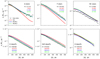 |
Fig. 9. Vertical number density profiles of the six local Gaia samples. The data are plotted with black crosses. The solid red and blue curves show predictions of the standard and MCMC1 JJ models. The number density profiles of the MCMC2 model are shown with dashed green lines. The observed and modelled number of stars in each sample are given with the same colour coding. The scale and range of y-axis are chosen different for all panels in order to show clearly the shapes of all profiles. |
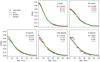 |
Fig. 10. Observed and predicted functions for the five Gaia kinematic samples from Table 1. As in Fig. 9, the data are plotted with black crosses, and the three coloured curves correspond to the model predictions. The observed and modelled number of stars in each sample are also given with the same colour coding. |
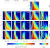 |
Fig. 11. Observed and predicted smoothed apparent Hess diagram of the Gaia conic sample. Four rows (top to bottom) show the data and predictions of the standard, the MCMC1, and the MCMC2 models. The contributions of the thin and thick disk as well as of the halo are shown in three columns on the left. Values given there in parenthesis correspond to each component’s relative contribution to the total Hess diagram in terms of star counts. The fourth column shows the total Hess diagram, where the observed or modelled number of stars is given in parentheses. The last column displays the logarithmic χ2 calculated according to Eq. (28). |
The vertical kinematics of the five Gaia samples is illustrated in Fig. 10. Again, the observed and predicted quantities, the normalised vertical velocity distributions f(|W|), are plotted with black crosses and coloured lines, respectively. As expected, there are non-negligible deviations between the data and the standard model (red curves) also in terms of kinematics. The main discrepancy reveals itself for the MS stars, where the mismatch between the relative fractions of dynamically cold and warm stars is quite significant. This feature was already reported by us in Sysoliatina et al. (2018a), where we also found that this effect is most pronounced close to the Galactic plane. Additionally, we observe a small imbalance between the fractions of dynamically cold and warm stars for the F-star sample (the relative ratio of dynamically cold stars is slightly overestimated in the model). In the case of the RC sample, the situation is reversed: the predicted relative fraction of dynamically cold stars is somewhat too low in the standard model.
Finally, we look at the apparent Hess diagram of the stars observed within the conic volume (Sect. 2.1.5). Constructed according to the recipe explained in Sect. 4.3, the Hess diagram is displayed in Fig. 11. Different panels in each row show the contributions from the thin disk, thick disk, and halo, as well as the total predicted Hess diagram and the logarithmic χ2 calculated according to Eq. (28). Different rows correspond to the data (Fig. 4, shown here for a visual comparison) and the standard, MCMC1 and MCMC2 JJ models. In the case of the standard model, the most important discrepancies between the modelled and observed apparent Hess diagram are located in the triangular area at GBP − GRP ≈ 0.6−0.7 mag and G ≈ 16−17 mag. This discrepancy originates from the halo component and is likely to be caused by an overestimated halo surface density. Another feature corresponding to the poor model-to-data consistency is observed at the bright end, for G ≈ 12−15 mag and GBP − GRP ≈ 0.8 mag. This can be attributed to the overestimated star counts of the thin-disk component. The flawed consistency at GBP − GRP ≈ 1 mag and G ≈ 14−17 mag can be related to both the thin- and thick-disk components. Additionally, the standard model performance in the GBP − GRP > 2 mag regime is also not perfect and we relate this to the mismatch of the lower-MS slope between the data and isochrones. We note that the vertical stripes at GBP − GRP ≈ 1.5, 1.7, 1.9 that are seen for the model predictions constructed with the PARSEC isochrones are related to the interpolation scheme of the stellar evolution code and not to the model features.
The described picture, when viewed as a whole, implies that several changes need to be made in order to improve the model’s performance. The inconsistencies seen over the Hess diagram in Fig. 11 indicate that the surface densities of the model components need to be adjusted. To improve the vertical profiles of A and F stars, a significant fraction of young stars with ages of τ ≲ 4−5 Gyr has to be added to the standard JJ model. However, simply adding more young stars cannot resolve the problem, as it is not just the number of A and F stars but also the shapes of their vertical profiles that have to be adjusted. In the case of the A-star sample the required profile adjustment is quite significant at |z|≳300 pc. The revealed difference between the observed and predicted A-star vertical profiles means that a small fraction of the youngest population represented by A stars is more dynamically heated than prescribed by the model AVR. A simple test shows that the observed vertical number density profile of A stars can be well fitted by a double-sechn profile. The main isothermal component of such fit (90% of the sample stars) has a velocity dispersion of ∼6 km s−1, similar to the value given by AVR for the youngest populations. However, the velocity dispersion of the second isothermal component has to be ∼12 km s−1, namely, twice as large. This is what motivated us to add a recent peak to the thin-disk SFR with the assumed mean age of τp2 ≈ 0.5 Gyr9 corresponding to the typical age of A stars (Fig. 8). Through the analogy to A stars, we added another SF burst centered at older ages, τp1 ≈ 3 Gyr, which may help to improve model-to-data consistency for the F-star sample. We also decouple the vertical velocity dispersions σp1 and σp2 of the young populations associated with the two added SF bursts from the thin-disk kinematics prescribed by the monotonous AVR. Here, the fraction of the thin-disk populations associated with the SF burst at a given Galactic time is defined as a ratio of the SFR function with a peak relative to a monotonously decreasing SFR. In terms of the definitions given by Eqs. (10) and (12), this is given as  . Finally, we decided to adapt two AVR parameters in order to improve the velocity distributions f(|W|) and the IMF parameters as the latter is naturally entangled with the SFR.
5.3.2. MCMC1 model
In the case of the optimised JJ model MCMC1, most of the issues described above are either resolved or relaxed.
The predicted number density profiles calculated with the new parameter values (Table 4) are shown in Fig. 9 with blue curves. The vertical profiles of A and F stars are now much better reproduced, also the underestimation in their overall star counts is reduced to ∼7% and ∼11%, respectively. The vertical profiles of the MS stars became somewhat steeper (G- and G/K-dwarf samples), and follow the observed trends more closely. The overall excess in the predicted number of stars for these two MS samples is reduced to ∼10% and ∼6%, respectively. Also, the MCMC1 model is more consistent with the data in terms of the vertical kinematics of the local stars. The corresponding modelled velocity distribution functions are shown in blue in Fig. 10. The velocity distributions f(|W|) of F and RC stars match the observed distributions perfectly, and in the case of the G-, G/K-, and K-dwarf samples, the model-to-data fit is noticeably improved. Additionally, almost all the aforementioned problematic areas at the apparent Hess diagram appear to be improved after the model calibration against Gaia. The overall star count model-to-data mismatch remains on the level of ∼6% (compare the second and third row in Fig. 11).
This improvement of the model performance is achieved as a result of several factors. Firstly, the model parameters are optimised in the high-dimensional space. Secondly, two additional SF bursts with the special vertical kinematics are added. Thirdly, the AMR of the model is adjusted to be consistent with the observed metallicity distribution of the local populations. We find that the Gaussian SF bursts centered at ages of ∼3 Gyr and ∼0.5 Gyr and characterised by the dispersions of ∼0.7 Gyr and ∼0.25 Gyr can significantly improve the model performance for the upper MS. The derived vertical velocity dispersions of the thin-disk stellar populations related to these episodes of the SF enhancement are ∼26 km s−1 and ∼12.6 km s−1, respectively. Using the positions, widths, and amplitude-related parameters of the two SF bursts from Table 4, we can calculate local surface densities of these thin-disk populations and find ∼1.8 M⊙ pc−2 and ∼0.27 M⊙ pc−2 for the older and younger bursts, respectively. Thus, these extra heated populations constitute ∼5.3% and ∼0.8% of the total disk surface density at the Solar circle.
The new SFR function with two recent SF bursts is displayed in Fig. 12. The thin- and thick-disk SFR, as well as the total SFR, are plotted in solid orange, green, and dashed black curves, respectively. The thin-disk SFR of the standard model is shown in blue and the magenta curve corresponds to the thin-disk SFR function presented in Paper I. We see that the new and original thin-disk SFR functions are fully consistent in terms of the overall decline and the only important difference between them is the presence of the recent SF bursts confirmed in this work.
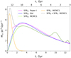 |
Fig. 12. Derived SFR function of the Galactic disk at the Solar circle. Orange and green curves show the thick- and thin-disk SFR calculated according to Eqs. (7) and (12) with the parameters of the MCMC1 model. The dashed black curve is the corresponding SFR of the total disk. The thin-disk SFR of the standard model is shown in blue. For comparison, we also plot the original thin-disk SFR from Paper I (magenta curve). |
Alongside the general model improvement, we report on the leftover model-to-data deviations. Among them, there is a mismatch between the observed and simulated RC star counts: the vertical profile and the overall star counts of the RC stars in the volume remain essentially the same after the model optimisation.
In the case of K dwarfs, the shape of the vertical profile is not improved and remains to be shallower than suggested by the Gaia data. From Fig. 11, we also see that the reddest part of the Hess diagram, GBP − GRP > 2 mag, populated by the faint low-mass K dwarfs, does not appear to be improved following the optimisation. Additionally, there is still a noticeable imbalance between the dynamically cold and hot MS populations of the disk (Fig. 10). The potential sources of these leftover discrepancies, their importance, as well as the model limitations and caveats are discussed below in Sect. 6.1.
5.3.3. MCMC2 model
The vertical number density profiles and W-velocity distribution functions predicted by the MCMC2 model are plotted as green dashed curves in Figs. 9 and 10, respectively. It is easy to see from these plots, as well as from Table 4, that the parameters and predictions of the models MCMC1 and MCMC2 are very close to being consistent. However, we cannot conclude that the stellar library does not have any impact on our stellar population synthesis as the apparent Hess diagram constructed with the MIST isochrones exhibits special features when compared to the predictions of the MCMC1 model (compare the third and fourth row in Fig. 11). It is obvious that the MIST isochrones give a less realistic model of the low-mass MS compared to the PARSEC code. It is for this reason that we mainly rely on the PARSEC stellar library and only use MIST isochrones for a complementary test.
5.3.4. Consistency test
The final step is performing a simple consistency test. We model the full local sample (Sect. 2.1.4) and compare it to the data over the absolute Hess diagram. The Hess diagrams shown in Fig. 13 are constructed with the updated JJ models MCMC1 and MCMC2 (left column). The overplotted black and white contours mark the distribution of stars in the data. The right column of Fig. 13 shows the logarithmic χ2 calculated for both models according to Eq. (28).
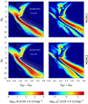 |
Fig. 13. Absolute Hess diagram of the full local sample (left column) as predicted by the MCMC1 and MCMC2 models (top to bottom). The black and white contours are added for comparison and show the distribution of stars in the data. The overplotted values give the total predicted number of stars in the sample and its relative difference to the observed number of stars. The right column shows the corresponding logarithmic χ2. |
Again, we see that the MCMC1 model gives a fully realistic representation of the data: a comparison of the observed and modelled MS positions (Fig. 13, upper left panel) shows that they are in good agreement with each other. The total number of the observed and predicted stars agrees within ∼5%, with a slight deficit of stars in the model relative to the data. The corresponding χ2 plot (Fig. 13, upper right panel) reveals a part of the MS that is severely underpopulated in the MCMC1 model (red stripe along the MS). However, this feature is expected as it originates simply from the fact that the modelled MS is narrower than the real one. This happens because we do not model binaries located right above the MS, and (to a lesser degree) because no metallicity scatter is added to AMR. The remaining inconsistency between the low-mass MS slopes is attributed to the properties of the PARSEC stellar library.
The predictions of the MCMC2 model (Fig. 13, second row) have the same features, but as we already expected based on its predictions of the K-dwarfs vertical number density profiles (Fig. 9) and the apparent Hess diagram (Fig. 11, last row), its overall model-to-data consistency in terms of the observed and modelled MS slopes is worse than in the case where PARSEC isochrones are used. Additionally, with regard to the lower-MS slope problem, we see that the modelled MS is shifted to the blue by ∼0.1 mag.
6. Discussion
6.1. Limitations and caveats
Before discussing the most interesting result of this work, the reconstructed SFR, we address potential limitations of our approach and estimate their possible impact on our findings.
6.1.1. Modelling approach
The most important limitation of our study is related to the way we define the SF history of the disk. Firstly, we assumed a parallel evolution of the thick and thin disk, which might not necessarily be the case. There are also two-infall models discussed in the literature (e.g. Grisoni et al. 2018) and more complicated scenarios where the thin- and thick-disk components form sequentially, one after another, with a transfer at ∼8 Gyr ago (Haywood et al. 2013). Secondly, we did not allow for a variation of the shape of the thick-disk SFR, but we simply scaled it with the Σt parameter. However, this should not be a significant limitation as the assumed duration of thick-disk formation is relatively short and in this case, the exact shape of the SFR function is not important. Finally, we define the thin-disk SFR in a parametric way and allow only two recent SF bursts inspired by the observed discrepancies between the Gaia data and the JJ model with a declining SFR. In reality, the SFR shape may be more complicated, with a number of peaks and dips which our present model does not account for. However, we tried to adapt many of the SFR parameters in order to vary its shape with as much freedom as it is possible within our framework.
In addition, we highlight once more that no explicit radial migration process is introduced in the current version of the JJ model. Although the new model parameters predict a better consistency between the model and data in terms of vertical kinematics, we still see a small imbalance between dynamically cold and hot stars in the model. This may point to a more complicated AVR shape than a simple power-law function increasing with stellar age as suggested by Eq. (13). Since dynamically cold stars are more likely to migrate, it is possible that there is a surplus of them in the data, which would correspond to a more pronounced core in the f(|W|) distributions than our model predicts.
6.1.2. Distances
Another source of uncertainty in this study is related to the data selection process. As we explained in Sect. 2.1.2, we adopt inverse parallaxes as stellar distance estimates and use them to calculate the absolute G-magnitudes as these are needed for the sample selection. Thus, our sample statistics directly depends on the adopted distance set. In Sysoliatina et al. (2018a) we used TGAS astrometric data with relative parallax errors as large as 30% at |z| = 1 kpc. As we show, in order to construct robust stellar density profiles and Hess diagrams, a parallax error model has to be included into the analysis. However, a proper modelling of the distance errors is challenging and significantly complexifies stellar population synthesis. We also want to avoid any distance quality-related cuts as these are known to introduce distance-dependent biases (Luri et al. 2018), which can be also challenging to model. Alternatively, Bayesian distances similar to those derived in Bailer-Jones et al. (2018) or McMillan (2018) can be used instead of inverse parallaxes. However, they should be used with caution, as the Galactic model used as a prior for Bayesian distances can be inconsistent with our Galactic model, which would eventually bias our model parameters. Ideally, only the Bayesian distances that were derived with this very model as a prior can be safely used to improve a Galactic model. In practice, this re-calculation of distances for each model parameter set during the model optimisation is hardly feasible and, therefore, a compromise between the calculation efficiency and a robustness of the approach should be found to perform a Galactic model calibration over the large volumes. At a minimum, additional tests have to be performed to check the models’ consistency and estimate the impact of different Bayesian distance sets on the model predictions.
At the same time, such Bayesian distances as those derived for the bright APOGEE RC stars and used in this work can be very helpful as they rely on the spectrophotometric modelling of the observed sample and do not depend on the assumptions about matter distribution across the Galactic disk. For the local volume considered in this work, any Bayesian distances will be very similar to the inverse parallaxes that we used here, therefore, distance uncertainties are not expected to influence our results. However, these considerations are of great importance for our future work, where the JJ model is to be applied to larger volumes.
6.1.3. Stellar evolution library
As we emphasise throughout this paper, our stellar population synthesis is naturally sensitive to the choice of the stellar evolution library. Two sets of the best model parameters in Table 4, obtained in the identical MCMC simulations based on the PARSEC and MIST isochrones, show the impact of the stellar library on our results. In general, the parameter values differ only slightly between the MCMC1 and MCMC2 models, typically by ∼0.3Δθ. Both runs indicate that the local stellar populations as observed by Gaia are inconsistent with a monotonously declining thin-disk SFR and two recent episodes of the enhanced SF are required to reproduce these data in our model framework. However, there are several problems related to the stellar libraries that influence the quality of our modelling.
For both PARSEC and MIST isochrones, we find a significant difference between the predicted and observed MS slope in the low-mass regime that corresponds to our K-dwarf sample and the reddest part of the apparent Hess diagram for stars in the cone, GBP − GRP ≳ 1.5−2 mag. In the case of MIST isochrones, this mismatch is quite severe (Figs. 11 and 13, bottom rows) and this is the reason why we chose this stellar library for a complementary test only and we treat the best model parameters obtained on its basis as less trustworthy. On the other hand, the MIST code has a better interpolation scheme than PARSEC, which is clearly demonstrated in Fig. 8. However, the lack of smoothness over the CMD in the case of PARSEC isochrones does not lead to any additional problems. Another issue that is possibly related to theoretic stellar evolution is the discrepancy between the modelled and observed RC star counts. Figure 9 shows that our model is able to reproduce the realistic vertical fall-off of the RC density, however, the mismatch in the number of stars remains significant, ∼33%, and does not decrease after the model optimisation. We suggest that this large difference can be related to the existing uncertainty in the lifetimes of core He-burning stars (Jones et al. 2015), and, therefore, it should not be overinterpreted. However, other possibilities have not been discarded, such as the observed difference in the density of giants, which may indicate that the shapes of the local SF history or AVR function are more complicated than those proposed in this work.
6.1.4. Dust model
As our Gaia sample selection relies on the de-reddened colours and magnitudes, it is intrinsically sensitive to the assumed 3D model of dust distribution. In order to investigate how the choice of the dust model influences our samples statistics, we tested two different dust maps: a high-resolution dust model from Green et al. (2019) complemented at ∼1/4 of the sky by the lower-resolution dust map from Lallement et al. (2018), and the Lallement et al. (2018) dust map applied for the whole sky. We found that the number of stars in the samples changes by a few % only, so this does not lead to any significant changes in the shapes of their vertical number density profiles and velocity distributions and, therefore, it can hardly affect our derived parameter values. An example of the impact of the extinction map on the F-star sample statistics is shown in Appendix B.
6.1.5. AMR
In Sect. 4.5, we made several simplifying assumptions to derive the AMR from the modelled RC ages and the observed metallicity distributions of the APOGEE stars.
In particular, we assumed that there is a direct and unique correspondence between stellar metallicities and ages, which in reality is not the case. Numerous studies based on photometric or spectroscopic metallicities and isochrone or chromospheric age estimates report a significant, ≳0.1 dex, metallicity scatter at all ages (Rocha-Pinto et al. 2000a; Haywood 2006; Casagrande et al. 2011) that looses the correlation between age and metallicity. For example, in Bergemann et al. (2014) the authors used Gaia-ESO abundances and did not find any significant age-metallicity correlation for stars younger than 8 Gyr in the extended Solar neighbourhood. The large scatter in metallicity cannot be entirely assigned to the effect of random errors of spectroscopic observations, but partly has physical origin: the effect of radial migration leads to mixing of stars from different radial zones in the Galactic disk and this partly smears out the age-metallicity correlation at each radius. In this study, we ignored the physical scatter in the AMR for the sake of saving computational time. Indeed, adding a scatter on top of the AMR implies that the number of stellar assemblies increases. This can noticeably stretch the calculation time required to achieve a reliable constraint on the model parameters (Sect. 4.6). On the other hand, adding a scatter in metallicity is expected to have a negligible impact on our results in the end: features on the synthetic CMD can only become smoother, but the number of stars in our wide colour-magnitude boxes used for the sample selection remains essentially unchanged.
Additionally, the most metal-rich parts of the high- and low-α populations of the RC APOGEE sample were removed from our AMR reconstruction process. Instead, we later add them to the predicted metallicity distributions in the form of the Gaussian error model. However, we cannot exclude the possibility that these high values of metallicity are realistic – and not artifacts produced by the pipeline routine applied to the range of metallicities where hardly any standard stars are known. In this case, a small fraction of our mock stellar populations, of ages τ ≲ 1.0 Gyr, have metallicites underestimated by up to ∼0.2 dex. This may have several implications for the population synthesis. The youngest dwarfs are located at the right (red) brim of the MS on the CMD. As increase in metallicity shifts an isochrone to redder colour, this means that in the case of an underestimated metallicity of the youngest stars, the width of our predicted MS is also slightly underestimated. For the F-star region on the CMD, the situation is inversed: the youngest F stars lay at the blue edge of the upper MS and, therefore, an underestimation of their metallicities means that the edge of the upper MS is shifted to bluer colours. Similarly, the RC population will appear too blue if the metallicity of its youngest stars is underestimated. However, none of these potential biases on the predicted CMD can introduce any significant difference to our sample statistics. Our colour-magnitude windows are wide enough so that small shifts of the MS and other CMD features cannot result in any significant change in the number of stellar assemblies falling into them. Therefore, an influence of this assumption on our final results is negligible.
6.2. Local star-formation history
The SFR of the Solar neighbourhood, as a key ingredient of dynamical and chemical evolution models, was probed in many studies with different techniques. However, there is still no full consistency between the results of these attempts.
Aumer & Binney (2009) used the local MS and turn-off stars common between HIPPARCOS and GCS, and simultaneously constrained the local kinematics and the SFR. To do so, they fitted the observed B − V colour distributions while assuming a disk heating function that monotonously increases with age along with the IMF from Kroupa et al. (1993), with its slope for m > 1 M⊙ varied in a small range around −2.7. They also adopted a reddening model from Vergely et al. (1998), corrected for the sample incompleteness, and used Padova isochrones to account for the stellar evolution. They tested different SFR shapes, including single- and double-exponential forms, a non-exponential decline, and a smooth SFR with an overlaid oscillatory component. These authors found that the irregular SFR is not favoured in their analysis and their best fit suggests an exponentially declining SFR. Similar results were obtained by Bovy (2017). In this study, a local sample from the TGAS catalogue of the Gaia DR1 was investigated and the long-lived K dwarfs were used to reconstruct the local SF history. The observed luminosity function of the sample was converted to the mass function, assuming the IMFs from Kroupa (2001) and Chabrier (2001), which was then used to derive the local SFR with the help of MS lifetimes and correction for the disk thickness. The author found that the local SFR reconstructed from the TGAS data can be perfectly fitted with an exponentially declining law, consistently with Aumer & Binney (2009). Another interesting study was presented in Snaith et al. (2015), where the time evolution of [Si/Fe] was used as a marker of the SF history. For the inner disk, R ≲ 8 kpc, their best-fit SFR has a strong peak at ages 10−12 Gyr and about 1 Gyr quenching period 8 Gyr ago, followed by a quasi-linear behaviour for the last 7 Gyr. This result was found to be insensitive to the variation of different parameters of the assumed chemical evolution model, including the IMF shape. Xiang et al. (2018) presented a study based on a sample of ∼1 million MS turn-off and subgiant stars from the LAMOST Galactic Survey with determined Bayesian isochrone ages. The authors performed a detailed reconstruction and analysis of the 3D stellar mass distribution of mono-age populations across the Galactic disk. They fitted vertical stellar distributions with sechn profiles and used the obtained scale heights to convert mid-plane mass densities to the present-day surface density as a function of age. With stellar evolution taken into account, this gives the SFR at different Galactocentric distances. Their SFR at R = 8 kpc has a peak ∼6 Gyr ago and declines monotonously up to the present day. Frankel et al. (2019) studied the APOGEE RC stars in a wide range of Galactocentric distances, 6 kpc < R < 13 kpc, and derived a radially dependent SFR of the α-low disk, with radial migration and chemical enrichment included in a parametric form. Their SFR was prescribed to cover the last 8 Gyr in age and follow an exponential law, thus, it was not possible to investigate the SFR shape in this study, as it was fixed. But an interesting outcome of this modelling is a prediction of an inside-out growth of the disk − a formation scenario that can successfully reproduce elemental abundances across the disk (Chiappini et al. 2001; Colavitti et al. 2009; Grisoni et al. 2018).
On the other hand, there are a number of works that report a complicated, non-monotonous behaviour of the local SFR for the last 5−6 Gyr. Hernandez et al. (2000) used Bayesian technique to reproduce the CMD of the HIPPARCOS complete volume-limited sample and determined the local SF history over the last 3 Gyr with a high 50 Myr resolution. The authors found that the reconstructed SFR can be represented as a constant continuum with an oscillatory component with a period of 0.5 Gyr. Rocha-Pinto et al. (2000b) derived the local SFR by applying the scale-height, stellar-evolution, and volume corrections to chromospheric ages of 552 late-type dwarfs. The obtained SFR has several episodes of SF enhancement, at 0−1 Gyr, 2−5 Gyr, and 7−9 Gyr ago, with the oldest burst being uncertain. Quite a different result was obtained by Cignoni et al. (2006) who used bright HIPPARCOS stars within 80 pc from the Sun and performed a Bayesian fit of the observed CMD with an MCMC technique. The recovered SFR relies on the Pisa evolutionary library (Cariulo et al. 2004), a power-law IMF with a slope −2.35, and the AMR as observed for GCS stars within 40 pc from the Sun. Their best SFR is essentially bimodal: epochs of enhanced SF are present for ages 2−6 Gyr and 10−12 Gyr, with the recent burst ∼2 times more enhanced than the older one. This result is consistent with the SFR determined by Vergely et al. (2002), where a very similar Bayesian inversion technique was applied to HIPPARCOS stars. A bimodal SFR was also obtained by Rowell (2013). They constrained the SFR by fitting the SDSS white-dwarf luminosity function and found broad SF peaks at 2−3 Gyr and 7−9 Gyr ago. A comparable result was recently presented by Bernard et al. (2018), where a recovered dynamically evolved SFR demonstrates peaks at ages of 14 Gyr and 2−3 Gyr. Again, this analysis was based on fitting the present-day CMD, which was constructed with the TGAS stars within 250 pc from the Sun. The best fit was based on the BaSTI stellar evolution library (Pietrinferni et al. 2004), and a correction for the disk thickening was applied to extrapolate the result to the whole local cylinder.
To sum up, most of the authors agree that there was a SF peak in the remote past, 10−14 Gyr ago. A number of authors also agree that there were one or multiple SF enhancement epochs during the last ∼6−7 Gyr, though the relative weights of the early and recent SF peaks are quite different in different studies. We can mention several reasons for this variety among the results. Different authors often use different stellar evolution libraries, applying different IMF, AVR, and kinematics as ingredients of their dynamical or chemical evolution models used to fit the observed quantities. Also many studies are based on stellar ages, which are known to be challenging to constrain. As a result, the time resolution of SFR may be limited, and the SFR shape can be distorted due to systematic errors that affect ages. Commonly, only a small number of model parameters are fitted simultaneously, the influence of other ingredients such as the IMF and disk heating is tested post factum, which may also lead to non-robust results if the multidimensional PDF in the full parameter space has a complicated shape, which cannot be known in advance and revealed with a small number of tests.
Our best total-disk SFR shown in Fig. 12 can be viewed as broadly consistent with studies of Snaith et al. (2015), Cignoni et al. (2006), Rowell (2013), and Bernard et al. (2018) as we also see two epochs of active star formation. However, our results do not agree with regard to the details concerning the shape of the overall SFR continuum. When compared to Aumer & Binney (2009) and Bovy (2017), we confirm their reported decline of the SFR to the present day, however, in our case, the exact shape of this decline is non-monotonous and non-exponential. The positions of the three SFR peaks reported by Rocha-Pinto et al. (2000b) are comparable to our two recent SF bursts and a weak peak ∼9.5 Gyr ago due to maximum contribution from the thin-disk star formation. We also confirm the result presented in Mor et al. (2019) as our SF peak centered at τ ≈ 3 Gyr is very similar to the one found in their study; a recent SF enhancement at τ ≈ 0.5 Gyr found by us could not be recovered by Mor et al. (2019) due to their limited age resolution. Finally, our SFR is not consistent with the local SFR from Xiang et al. (2018) as both the global shape and small time-scale behaviour of two SFR functions are very different.
Is is necessary to stress here that most of the parameters characterising these recent SF bursts are found quite difficult to constrain within our framework. Thus, some uncertainty still remains with respect to the exact shape and duration of the SF enhancement periods. According to our results, which show, for example, that the most recent epoch of the enhanced SF may be actively happening now as τp2 ≈ 0 Gyr is not excluded (see the likelihood PDF for this parameter in Fig. C.1).
Finally, we find it necessary to put our results in the framework of the radial migration problem. As we mentioned in Sect. 1, our local SFR can be roughly viewed as a disk formation history averaged over a radial annulus R⊙ ± ΔR, where ΔR represents the effect of the radial migration and may be significantly larger than the half-width of the local annulus of 0.15 kpc, where the data were selected (Sect. 2.1.2). However, this is a simplified picture as we know that the radial migration effect accumulates with time, such that the oldest populations observed locally are expected to be significantly more contaminated by migrators than the youngest ones. If we adopt the radial migration strength of 2.6  from Frankel et al. (2020), then for the mean ages of our recent SF bursts of 0.5 Gyr and 3 Gyr, we get ∼0.75 kpc and ∼1.8 kpc. It is easy to convert this to the distributions over Rbirth within the local annulus R⊙ ± 0.15 kpc, for simplicity assuming an exponential radial density fall-off with the scale length of 2.0 kpc (consistent with the value for the metal-rich thin-disk population found by us in Sysoliatina et al. 2018b). Due to the negative density gradient with R, local Rbirth distributions will be shifted towards the inner disk, with older stars representing, on average, smaller R: for τ = 0.5 Gyr distribution peaks at ∼8 kpc, and for τ = 3 Gyr the peak is at ∼7.4 kpc. From the cumulative distributions, we estimate that 68% of the local 0.5 Gyr and 3 Gyr old stars were born within ∼0.55 kpc and ∼1.5 kpc from R⊙, respectively. Thus, the additional assumption on the strength of radial migration does not disprove our findings, but simply gives us an idea of the range of Galactocentric distances represented by our ‘local’ SFR at the given ages.
The recent epochs of an increased SF activity in the Solar neighbourhood recovered in our study may indicate the recent gas infall episodes. Also, the most recent increase of the SF may result from an increase of the SF efficiency related to an exhaustion of the local gas reservoir. In order to put more constraints on the recent SFR and clarify the origin of the SF bursts, a further and in-depth study of the local young populations is required.
7. Conclusions
In this work, we present an updated version of our semi-analytic dynamic model of the Milky Way disk. The new features of the the JJ model are summarised in the following:
-
We introduced a new simple gas model that consists of two isothermal populations representing molecular and atomic gas components. They are characterised by the local surface densities and scale heights that are adopted from McKee et al. (2015) and Nakanishi & Sofue (2016), respectively.
-
We linked the W-velocity dispersion of a zero-age thin-disk stellar population to the W-velocity dispersion of the molecular gas, with the latter determined during an iterative solving of the Poisson-Boltzmann equation. This allows us to set a constraint on one of the AVR parameters and, therefore, to reduce the total number of free parameters in the model.
-
Assuming a parallel evolution of the thin and thick disk, we defined an extended in time thick-disk SFR. It has a rapid power-law increase, peaks at age of ∼12.5 Gyr and declines exponentially, such that the thick-disk SF drops to zero ∼10 Gyr ago (Fig. 12, orange curve).
-
A new power-law analytic form of the thin-disk SFR is presented, such that the new JJ model with an updated disk treatment is consistent with the results of the previous works in this series, Paper I-Paper III. We also allowed two recent SF bursts at ages 0−1 Gyr and 2−4 Gyr added to the thin-disk SFR in the form of Gaussian peaks. Additionally, in order to reproduce the observed vertical number density trends of A and F stars, we decoupled the vertical kinematics of the thin-disk populations associated with the assumed SF bursts from the kinematics of the rest of thin-disk populations prescribed by the AVR. To do so, we introduced parameters, σp1 and σp2, which give the W-velocity dispersion of the stellar populations associated with the SF excess during the recent epochs of the enhanced SF.
We used stars from Gaia DR2 selected with simple colour-magnitude cuts on the CMD. The six samples included young stars of A and F spectral classes, mixed-age sample dominated by RC giants, and three sets of the long-lived G and K dwarfs probing the lower MS region. An additional sample of Gaia stars was selected in two cones directed towards the northern and southern Galactic poles (see Sect. 2.1 and Table 1).
Using the local APOGEE RC stars, we constrained the AMR in the Solar annulus, assuming a separate chemical evolution of the thin and thick disk (Fig. 6). The derived AMR is used in the stellar population synthesis with the PARSEC stellar library. Then, working within a Bayesian framework, we simultaneously optimised the JJ model performance in terms of the vertical kinematics and number density profiles of the selected populations, as well as in terms of the apparent Hess diagram of the conic sample. We searched for a maximum probability region in a multidimensional model parameter space using the MCMC technique and self-consistently constrained 22 model parameters. These parameters include the local surface densities of the four Galactic components, thin- and thick-disk vertical kinematics, the shape of the IMF, and the thin-disk SFR function. These derived parameter values were also brought into consistency with the model-dependent AMR constrained with the APOGEE data.
We find that a monotonously declining SFR is inconsistent with the Gaia data and the observed local star counts imply two SF bursts in the recent past centered at ages ∼0.5 Gyr and ∼3 Gyr. These bursts are characterised by ∼30% and ∼55% increase of the SF relative to the underlying declining continuum, respectively. The thin-disk stellar populations associated with this SF excess were found to have W-velocity dispersions of ∼12.5 km s−1 and ∼26 km s−1, which is ∼1.8 times higher than the velocity dispersion prescribed by the monotonously declining AVR for the thin-disk populations of the same age. The relative contribution of these heated populations to the overall local surface density of the disk is estimated as ∼0.8% and ∼5.3%. The new local JJ model is able to reproduce the overall star counts with ∼5% accuracy for |z|≲600 pc (Fig. 13) and with ∼6−8% accuracy in the conic volume towards the Galactic poles (Fig. 11).
In summary, the spatial distribution and motions of the local stars as observed by Gaia can be well reproduced within a framework of our plane-symmetric semi-analytic model and a calibration of the model against the high-quality astrometric and spectroscopic data reveals previously unknown details of the Milky Way’s disk evolution.
Indices 2, 3, and 6 in the column names of Table 1 refer to the number of the phase space components known for a given sample.
We use Gaia ARI TAP services at http://gaia.ari.uni-heidelberg.de/tap.html
https://stilism.obspm.fr/. An updated version of the map has been recently presented in Lallement et al. (2019) where Gaia parallaxes were used as a proxy of distance to the APOGEE target stars, but this new dust map is not yet available in Stilism.
Acknowledgments
This work was supported by the Deutsche Forschungsgemeinschaft (DFG, German Research Foundation) – Project-ID 13871353 – SFB 881 (‘The Milky Way System’, subproject A06). This work has made use of data from the European Space Agency (ESA) mission Gaia (https://www.cosmos.esa.int/gaia), processed by the Gaia Data Processing and Analysis Consortium (DPAC, https://www.cosmos.esa.int/web/gaia/dpac/consortium). Funding for the DPAC has been provided by national institutions, in particular the institutions participating in the Gaia Multilateral Agreement. Besides the software mentioned in the text, this research made use of Python packages SciPy (Virtanen et al. 2020) and NumPy (Van Der Walt et al. 2011), a Python library for publication quality graphics matplotlib (Hunter 2007), a community-developed core Python package for Astronomy Astropy (Astropy Collaboration 2013, 2018), a Python mini-package fast-histogram (https://github.com/astrofrog/fast-histogram), as well as an interactive graphical viewer and editor for tabular data TOPCAT (Taylor 2005). We also thank Jan Rybizki for the helpful discussion and Alex Razim for many useful comments on the paper structure and tips on the text style. Finally, we thank organisers of the inspiring seminar ‘The Science Cloud’ (12-15.01.2020, Bad Honnef, Germany) funded by the Wilhelm and Else Heraeus-Foundation.
References
- Argast, D., Samland, M., Gerhard, O. E., & Thielemann, F.-K. 2000, A&A, 356, 873 [NASA ADS] [Google Scholar]
- Astropy Collaboration (Robitaille, T. P., et al.) 2013, A&A, 558, A33 [NASA ADS] [CrossRef] [EDP Sciences] [Google Scholar]
- Astropy Collaboration (Price-Whelan, A. M., et al.) 2018, AJ, 156, 123 [Google Scholar]
- Aumer, M., & Binney, J. J. 2009, MNRAS, 397, 1286 [Google Scholar]
- Bahcall, J. N. 1984, ApJ, 276, 156 [Google Scholar]
- Bailer-Jones, C. A. L., Rybizki, J., Fouesneau, M., Mantelet, G., & Andrae, R. 2018, AJ, 156, 58 [NASA ADS] [CrossRef] [Google Scholar]
- Bailer-Jones, C. A. L., Fouesneau, M., & Andrae, R. 2019, MNRAS, 490, 5615 [Google Scholar]
- Ban, M., Kerins, E., & Robin, A. C. 2016, A&A, 595, A53 [Google Scholar]
- Bennett, M., & Bovy, J. 2019, MNRAS, 482, 1417 [NASA ADS] [CrossRef] [Google Scholar]
- Bergemann, M., Ruchti, G. R., Serenelli, A., et al. 2014, A&A, 565, A89 [NASA ADS] [CrossRef] [EDP Sciences] [Google Scholar]
- Bernard, E. J. 2018, IAU Symp., 330, 148 [Google Scholar]
- Bienaymé, O., Leca, J., & Robin, A. C. 2018, A&A, 620, A103 [EDP Sciences] [Google Scholar]
- Bland-Hawthorn, J., & Gerhard, O. 2016, ARA&A, 54, 529 [NASA ADS] [CrossRef] [EDP Sciences] [Google Scholar]
- Bland-Hawthorn, J., Sharma, S., Tepper-Garcia, T., et al. 2019, MNRAS, 486, 1167 [Google Scholar]
- Bolatto, A. D., Wolfire, M., & Leroy, A. K. 2013, ARA&A, 51, 207 [Google Scholar]
- Bovy, J. 2017, MNRAS, 470, 1360 [Google Scholar]
- Bovy, J., Nidever, D. L., Rix, H.-W., et al. 2014, ApJ, 790, 127 [Google Scholar]
- Bressan, A., Marigo, P., Girardi, L., et al. 2012, MNRAS, 427, 127 [NASA ADS] [CrossRef] [Google Scholar]
- Cabral, N., Lagarde, N., Reylé, C., Guilbert-Lepoutre, A., & Robin, A. C. 2019, A&A, 622, A49 [Google Scholar]
- Cantat-Gaudin, T., & Anders, F. 2020, A&A, 633, A99 [NASA ADS] [CrossRef] [EDP Sciences] [Google Scholar]
- Cariulo, P., Degl’Innocenti, S., & Castellani, V. 2004, A&A, 421, 1121 [NASA ADS] [CrossRef] [EDP Sciences] [Google Scholar]
- Casagrande, L., Schönrich, R., Asplund, M., et al. 2011, A&A, 530, A138 [NASA ADS] [CrossRef] [EDP Sciences] [Google Scholar]
- Chabrier, G. 2001, ApJ, 554, 1274 [Google Scholar]
- Chen, B. Q., Huang, Y., Hou, L. G., et al. 2019, MNRAS, 487, 1400 [Google Scholar]
- Chiappini, C., Matteucci, F., & Romano, D. 2001, ApJ, 554, 1044 [Google Scholar]
- Choi, J., Dotter, A., Conroy, C., et al. 2016, ApJ, 823, 102 [Google Scholar]
- Cignoni, M., Degl’Innocenti, S., Prada Moroni, P. G., & Shore, S. N. 2006, A&A, 459, 783 [Google Scholar]
- Colavitti, E., Cescutti, G., Matteucci, F., & Murante, G. 2009, A&A, 496, 429 [NASA ADS] [CrossRef] [EDP Sciences] [Google Scholar]
- Cui, X.-Q., Zhao, Y.-H., Chu, Y.-Q., et al. 2012, Res. Astron. Astrophys., 12, 1197 [NASA ADS] [CrossRef] [Google Scholar]
- Czekaj, M. A., Robin, A. C., Figueras, F., Luri, X., & Haywood, M. 2014, A&A, 564, A102 [NASA ADS] [CrossRef] [EDP Sciences] [Google Scholar]
- de la Fuente Marcos, R., de la Fuente Marcos, C., Moni Bidin, C., Ortolani, S., & Carraro, G. 2015, A&A, 581, A13 [NASA ADS] [CrossRef] [EDP Sciences] [Google Scholar]
- de Salas, P. F., Malhan, K., Freese, K., Hattori, K., & Valluri, M. 2019, J. Cosmol. Astropart. Phys., 2019, 037 [Google Scholar]
- Dotter, A. 2016, ApJS, 222, 8 [NASA ADS] [CrossRef] [Google Scholar]
- Eisenstein, D. J., Weinberg, D. H., Agol, E., et al. 2011, AJ, 142, 72 [Google Scholar]
- Evans, D. W., Riello, M., De Angeli, F., et al. 2018, A&A, 616, A4 [NASA ADS] [CrossRef] [EDP Sciences] [Google Scholar]
- Flynn, C., Holmberg, J., Portinari, L., Fuchs, B., & Jahreiß, H. 2006, MNRAS, 372, 1149 [Google Scholar]
- Foreman-Mackey, D., Hogg, D. W., Lang, D., & Goodman, J. 2013, PASP, 125, 306 [Google Scholar]
- Frankel, N., Rix, H.-W., Ting, Y.-S., Ness, M., & Hogg, D. W. 2018, ApJ, 865, 96 [Google Scholar]
- Frankel, N., Sanders, J., Rix, H.-W., Ting, Y.-S., & Ness, M. 2019, ApJ, 884, 99 [Google Scholar]
- Frankel, N., Sanders, J., Ting, Y.-S., & Rix, H.-W. 2020, ApJ, 896, 15 [Google Scholar]
- Gaia Collaboration (Brown, A. G. A., et al.) 2016, A&A, 595, A2 [NASA ADS] [CrossRef] [EDP Sciences] [Google Scholar]
- Gaia Collaboration (Brown, A. G. A., et al.) 2018a, A&A, 616, A1 [NASA ADS] [CrossRef] [EDP Sciences] [Google Scholar]
- Gaia Collaboration (Katz, D., et al.) 2018b, A&A, 616, A11 [NASA ADS] [CrossRef] [EDP Sciences] [Google Scholar]
- Gravity, C., Abuter, R., et al. 2019, A&A, 625, L10 [NASA ADS] [CrossRef] [EDP Sciences] [Google Scholar]
- Green, G. M., Schlafly, E., Zucker, C., Speagle, J. S., & Finkbeiner, D. 2019, ApJ, 887, 93 [Google Scholar]
- Grisoni, V., Spitoni, E., & Matteucci, F. 2018, MNRAS, 481, 2570 [NASA ADS] [Google Scholar]
- Griv, E., Gedalin, M., Shih, I. C., Hou, L. G., & Jiang, I. G. 2020, MNRAS, 493, 2111 [Google Scholar]
- Haywood, M. 2006, MNRAS, 371, 1760 [Google Scholar]
- Haywood, M., Di Matteo, P., Lehnert, M. D., Katz, D., & Gómez, A. 2013, A&A, 560, A109 [NASA ADS] [CrossRef] [EDP Sciences] [Google Scholar]
- Hernandez, X., Valls-Gabaud, D., & Gilmore, G. 2000, MNRAS, 316, 605 [Google Scholar]
- Hunt, J. A. S., Bub, M. W., Bovy, J., et al. 2019, MNRAS, 490, 1026 [Google Scholar]
- Hunter, J. D. 2007, Comput. Sci. Eng., 9, 90 [NASA ADS] [CrossRef] [Google Scholar]
- Jahreiß, H., & Wielen, R. 1997, ESA SP-402: HIPPARCOS’97. eds. B. Battrick, M. A. C. Perryman, & P. L. Bernacca (Noordwijk: ESA), Presentation of the Hipparcos andTycho Catalogues and the First Astrophysical Results of the Hipparcos Space Astrometry Mission, 675 [Google Scholar]
- Jofré, P., Heiter, U., & Soubiran, C. 2019, ARA&A, 57, 571 [Google Scholar]
- Jones, S., Hirschi, R., Pignatari, M., et al. 2015, MNRAS, 447, 3115 [Google Scholar]
- Just, A., & Jahreiß, H. 2010, MNRAS, 402, 461 [Google Scholar]
- Just, A., Gao, S., & Vidrih, S. 2011, MNRAS, 411, 2586 [Google Scholar]
- Karakas, A. I. 2010, MNRAS, 403, 1413 [Google Scholar]
- Katz, D., Sartoretti, P., Cropper, M., et al. 2019, A&A, 622, A205 [NASA ADS] [CrossRef] [EDP Sciences] [Google Scholar]
- Khanna, S., Sharma, S., Tepper-Garcia, T., et al. 2019, MNRAS, 489, 4962 [Google Scholar]
- Khoperskov, S., Di Matteo, P., Gerhard, O., et al. 2019, A&A, 622, L6 [NASA ADS] [CrossRef] [EDP Sciences] [Google Scholar]
- Kounkel, M., & Covey, K. 2019, AJ, 158, 122 [Google Scholar]
- Kroupa, P. 2001, MNRAS, 322, 231 [NASA ADS] [CrossRef] [Google Scholar]
- Kroupa, P., Tout, C. A., & Gilmore, G. 1993, MNRAS, 262, 545 [Google Scholar]
- Kunder, A., Kordopatis, G., Steinmetz, M., et al. 2017, AJ, 153, 75 [Google Scholar]
- Lallement, R., Capitanio, L., Ruiz-Dern, L., et al. 2018, A&A, 616, A132 [NASA ADS] [CrossRef] [EDP Sciences] [Google Scholar]
- Lallement, R., Babusiaux, C., Vergely, J. L., et al. 2019, A&A, 625, A135 [NASA ADS] [CrossRef] [EDP Sciences] [Google Scholar]
- Lindegren, L., Lammers, U., Bastian, U., et al. 2016, A&A, 595, A4 [NASA ADS] [CrossRef] [EDP Sciences] [Google Scholar]
- Lindegren, L., Hernández, J., Bombrun, A., et al. 2018, A&A, 616, A2 [NASA ADS] [CrossRef] [EDP Sciences] [Google Scholar]
- Liu, L., & Pang, X. 2019, ApJS, 245, 32 [Google Scholar]
- Luri, X., Brown, A. G. A., Sarro, L. M., et al. 2018, A&A, 616, A9 [NASA ADS] [CrossRef] [EDP Sciences] [Google Scholar]
- Maíz Apellániz, J., & Weiler, M. 2018, A&A, 619, A180 [NASA ADS] [CrossRef] [EDP Sciences] [Google Scholar]
- Majewski, S. R., Schiavon, R. P., Frinchaboy, P. M., et al. 2017, AJ, 154, 94 [NASA ADS] [CrossRef] [Google Scholar]
- Maoz, D., Sharon, K., & Gal-Yam, A. 2010, ApJ, 722, 1879 [Google Scholar]
- Marigo, P., Girardi, L., Bressan, A., et al. 2017, ApJ, 835, 77 [NASA ADS] [CrossRef] [Google Scholar]
- Martell, S. L., Sharma, S., Buder, S., et al. 2017, MNRAS, 465, 3203 [Google Scholar]
- McKee, C. F., Parravano, A., & Hollenbach, D. J. 2015, ApJ, 814, 13 [NASA ADS] [CrossRef] [Google Scholar]
- McMillan, P. J. 2018, Res. Notes Am. Astron. Soc., 2, 51 [Google Scholar]
- Meingast, S., Alves, J., & Fürnkranz, V. 2019, A&A, 622, L13 [NASA ADS] [CrossRef] [EDP Sciences] [Google Scholar]
- Minchev, I., Anders, F., Recio-Blanco, A., et al. 2018, MNRAS, 481, 1645 [Google Scholar]
- Mor, R., Robin, A. C., Figueras, F., & Antoja, T. 2018, A&A, 620, A79 [Google Scholar]
- Mor, R., Robin, A. C., Figueras, F., Roca-Fàbrega, S., & Luri, X. 2019, A&A, 624, L1 [NASA ADS] [CrossRef] [EDP Sciences] [Google Scholar]
- Nakanishi, H., & Sofue, Y. 2016, PASJ, 68, 5 [Google Scholar]
- Nasello, G., Robin, A. C., Reylé, C., & Lagarde, N. 2018, in Rediscovering Our Galaxy, eds. C. Chiappini, I. Minchev, E. Starkenburg, & M. Valentini, 334, 347 [Google Scholar]
- Ness, M., Hogg, D. W., Rix, H. W., Ho, A. Y. Q., & Zasowski, G. 2015, ApJ, 808, 16 [Google Scholar]
- Nieva, M. F., & Przybilla, N. 2012, A&A, 539, A143 [NASA ADS] [CrossRef] [EDP Sciences] [Google Scholar]
- Nomoto, K., Kobayashi, C., & Tominaga, N. 2013, ARA&A, 51, 457 [Google Scholar]
- Nordström, B., Mayor, M., Andersen, J., et al. 2004, A&A, 418, 989 [NASA ADS] [CrossRef] [EDP Sciences] [Google Scholar]
- Ortolani, S., Held, E. V., Nardiello, D., et al. 2019, A&A, 627, A145 [Google Scholar]
- Paxton, B., Bildsten, L., Dotter, A., et al. 2011, ApJS, 192, 3 [Google Scholar]
- Paxton, B., Cantiello, M., Arras, P., et al. 2013, ApJS, 208, 4 [NASA ADS] [CrossRef] [Google Scholar]
- Paxton, B., Marchant, P., Schwab, J., et al. 2015, ApJS, 220, 15 [Google Scholar]
- Pietrinferni, A., Cassisi, S., Salaris, M., & Castelli, F. 2004, ApJ, 612, 168 [NASA ADS] [CrossRef] [Google Scholar]
- Read, J. I. 2014, J. Phys. G Nucl. Phys., 41, 063101 [NASA ADS] [CrossRef] [Google Scholar]
- Robin, A. C., Reylé, C., Derrière, S., & Picaud, S. 2003, A&A, 409, 523 [NASA ADS] [CrossRef] [EDP Sciences] [Google Scholar]
- Robin, A. C., Reylé, C., Marshall, D. J., & Schultheis, M. 2012, Astrophys. Space Sci. Proc., 26, 171 [Google Scholar]
- Robin, A. C., Reylé, C., Bienaymé, O., Fernandez-Trincado, J. G., & Amôres, E. B. 2016, Astron. Nachr., 337, 884 [Google Scholar]
- Robin, A. C., Bienaymé, O., Fernández-Trincado, J. G., & Reylé, C. 2017, A&A, 605, A1 [NASA ADS] [CrossRef] [EDP Sciences] [Google Scholar]
- Rocha-Pinto, H. J., Maciel, W. J., Scalo, J., & Flynn, C. 2000a, A&A, 358, 850 [NASA ADS] [Google Scholar]
- Rocha-Pinto, H. J., Scalo, J., Maciel, W. J., & Flynn, C. 2000b, A&A, 358, 869 [NASA ADS] [Google Scholar]
- Röser, S., Schilbach, E., & Goldman, B. 2019, A&A, 621, L2 [NASA ADS] [CrossRef] [EDP Sciences] [Google Scholar]
- Rowell, N. 2013, MNRAS, 434, 1549 [Google Scholar]
- Rybizki, J. 2018, ArXiv e-prints [arXiv:1802.08432] [Google Scholar]
- Rybizki, J., & Just, A. 2015, MNRAS, 447, 3880 [Google Scholar]
- Rybizki, J., Demleitner, M., Fouesneau, M., et al. 2018, PASP, 130, 074101 [Google Scholar]
- Rybizki, J., Just, A., & Rix, H.-W. 2017, A&A, 605, A59 [NASA ADS] [CrossRef] [EDP Sciences] [Google Scholar]
- Sanders, J. L., & Das, P. 2018, MNRAS, 481, 4093 [Google Scholar]
- Schönrich, R., & Binney, J. 2009, MNRAS, 396, 203 [Google Scholar]
- Schönrich, R., Binney, J., & Dehnen, W. 2010, MNRAS, 403, 1829 [NASA ADS] [CrossRef] [Google Scholar]
- Sellwood, J. A., & Binney, J. J. 2002, MNRAS, 336, 785 [Google Scholar]
- Skrutskie, M. F., Cutri, R. M., Stiening, R., et al. 2006, AJ, 131, 1163 [NASA ADS] [CrossRef] [Google Scholar]
- Snaith, O., Haywood, M., Di Matteo, P., et al. 2015, A&A, 578, A87 [NASA ADS] [CrossRef] [EDP Sciences] [Google Scholar]
- Sysoliatina, K., Just, A., Koutsouridou, I., et al. 2018a, A&A, 620, A71 [NASA ADS] [CrossRef] [EDP Sciences] [Google Scholar]
- Sysoliatina, K., Just, A., Golubov, O., et al. 2018b, A&A, 614, A63 [Google Scholar]
- Taylor, M. B. 2005, ASP Conf. Ser., 347, 29 [Google Scholar]
- Van Der Walt, S., Colbert, S. C., & Varoquaux, G. 2011, Comput. Sci. Eng., 13, 22 [Google Scholar]
- van Leeuwen, F. 2007, in Hipparcos, the New Reduction of the Raw Data, Astrophys. Space Sci. Library, 350 [Google Scholar]
- Vergely, J.-L., Ferrero, R. F., Egret, D., & Koeppen, J. 1998, A&A, 340, 543 [NASA ADS] [Google Scholar]
- Vergely, J. L., Köppen, J., Egret, D., & Bienaymé, O. 2002, A&A, 390, 917 [NASA ADS] [CrossRef] [EDP Sciences] [Google Scholar]
- Virtanen, P., Gommers, R., Oliphant, T. E., et al. 2020, Nat. Methods, 17, 261 [Google Scholar]
- Widrow, L. M., Barber, J., Chequers, M. H., & Cheng, E. 2014, MNRAS, 440, 1971 [Google Scholar]
- Wielen, R., Fuchs, B., & Dettbarn, C. 1996, A&A, 314, 438 [NASA ADS] [Google Scholar]
- Xiang, M., Shi, J., Liu, X., et al. 2018, ApJS, 237, 33 [NASA ADS] [CrossRef] [Google Scholar]
Appendix A: TAP queries
SELECT source_id, ra, dec, pmra, pmdec, parallax, radial_velocity,phot_g_mean_mag, bp_rp,
  ra_error, dec_error, pmra_error, pmdec_error, parallax_error, radial_velocity_error,
  dec_parallax_corr, dec_pmdec_corr, dec_pmra_corr, parallax_pmra_corr, parallax_pmdec_corr,
  pmra_pmdec_corr, ra_dec_corr, ra_parallax_corr, ra_pmdec_corr, ra_pmra_corr,
  phot_bp_rp_excess_factor, astrometric_excess_noise, astrometric_excess_noise_sig,
  RADIANS(b) as b_rad, RADIANS(l) as l_rad,
  QUAD(R⊙*R⊙ + COS(b_rag)*COS(b_rad)/parallax/parallax - 2*R⊙*COS(b_rad)*COS(l_rad)/parallax) as rg
FROM gaiadr2.gaia_source
WHERE AND phot_g_mean_mag > 7 AND phot_g_mean_mag < 17 AND bp_rp > 0 AND bp_rp < 3.3
  1000/parallax < 600 AND rg > 8.05 AND rg < 8.35
SELECT source_id, l, b, ra, dec, parallax, phot_g_mean_mag, bp_rp, phot_bp_rp_excess_factor
FROM gaiadr2.gaia_source
WHERE ABS(b) > 80 AND bp_rp > 0 AND bp_rp < 3.5 AND phot_g_mean_mag > 12 AND phot_g_mean_mag < 17
Appendix B: Impact of dust maps
We use a probabilistic extinction map constructed using Gaia parallaxes and photometry from 2MASS and PanSTARRS Green et al. (2019) (Fig. B.1, left panel). This map has a high resolution, on the order of ∼10′, and covers a large range of heliocentric distances, up to ∼10 kpc. However, it does not cover the whole sky, so we complement it with another 3D dust map from Lallement et al. (2018). This map is based on the APOGEE red giant stars with reddening estimated from Gaia and 2MASS photometry and photometric distances. It has significantly lower resolution and smaller spatial coverage: it extends 2 kpc away from the Sun in the Galactic plane, but goes only as high as |z| = 600 pc in the vertical direction. We downloaded the distance reddening curves using the online tool Stilism10 for 3072 line-of-sights that corresponds to the angular resolution of ∼3.66° (Fig. B.1, right panel). Both maps have similar large-scale features, but the map from Green et al. (2019) provides many small-scale details and, therefore, it is more preferable.
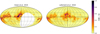 |
Fig. B.1. Extinction maps used in this study. Colour-coding displays the cumulative reddening up to 500 pc from the Sun. |
We selected our Gaia samples (Table 1) using both maps and then compare the sample statistics. We find that the overall number of stars in the samples may change by ∼4% maximum, with the largest impact observed for the F-star sample. Indeed, in the case of F stars we select a CMD region with a strong gradient in the stellar density (Fig. B.2, inset), such that a small shift along colour and magnitude axes due to a change in reddening and extinction leads to a significant change in the number of stars within this region. Figure B.2 shows that the corresponding difference in the vertical profile shape is small. We do not find any impact from this effect on the velocity distributions of our samples.
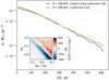 |
Fig. B.2. Vertical number density profiles of two F-star samples. The samples are selected in the colour-magnitude window defined in Table 1 using Gaia DR2 colours and magnitudes de-reddened with two different dust maps from Fig. B.1. The inset plot shows the absolute difference between these two F-star samples over the Hess diagram. |
In summary, changing the dust model may produce only a small impact on some of the analysed quantities and, therefore, this step would not influence the optimised values of the JJ model parameters determined in this work.
Appendix C: Full MCMC output
All Tables
All Figures
|
Fig. 1. Spatial geometry of the Gaia samples in XY projection (apart from the conic sample; see Sect. 2.1.5). The Galactic centre (GC) is marked with a black point. Each Gaia sample is selected in a Solar-centred spherical shell with the inner and outer radii of dmin and dmax from Table 1 (see columns d3 and d6 for the full samples and kinematic subsamples, respectively). Additionally, only stars belonging to the local annulus R⊙ ± ΔR with R = 8.2 kpc and ΔR = 150 pc are taken into consideration (thick grey arcs). |
| In the text | |
|
Fig. 2. Top row: selected samples of the local A, F, and RC stars and G and K dwarfs on the absolute CMD constructed with the de-reddened Gaia DR2 colours and magnitudes (left). Completeness of these samples as given by Eq. (4) over the CMD (middle) and across the sky (right). Bottom row: kinematic subsamples selected from the samples from the top row, except for A stars (left). Illustration of an additional incompleteness introduced by selecting only stars with available radial velocities (see Eq. (5)) and variation of this incompleteness over the CMD (middle) and across the sky (right). |
| In the text | |
|
Fig. 3. Spatial distribution of the six Gaia samples (top row) and their five kinematic subsets (bottom row) plotted in XZ Cartesian coordinates. The X axis points to the GC. |
| In the text | |
|
Fig. 4. Smoothed apparent Hess diagram of the conic sample constructed with the de-reddened Gaia DR2 colours and apparent magnitudes. |
| In the text | |
|
Fig. 5. Local low-α thin-disk (green) and high-α thick-disk (orange) samples selected for the analysis. The full APOGEE RC sample is shown in grey. The dashed black line marks the adopted boundary between the two populations, as in Eq. (6). |
| In the text | |
|
Fig. 6. AMR reconstruction. All model predictions shown here are generated with the best-fit parameters of MCMC1 model (Sect. 5). Left: normalised CMDFs of the high- and low-α APOGEE RC samples. Grey crosses show the smoothed data, thick black lines are the ‘deconvolved’ CMDFs (see text), and the full coloured lines illustrate the result of the convolution of the ‘deconvolved’ CMDF with Gaussian kernels. Middle: modelled CADFs for the thin and thick disk RC populations. Right: resulting AMR for the thin and thick disk. Analytic fits are over-plotted with black dashed curves. |
| In the text | |
|
Fig. 7. Posterior PDF marginalised over the least important parameters from the set θ. The probability distribution is sampled during the MCMC1 simulation. Thin grey lines mark the standard values of parameters θ0 and black crosses show their new best values. Histograms on the plot diagonal show each parameter PDF (coloured steps), Gaussian priors (dashed black curves), and the likelihood PDFs (light-blue steps). |
| In the text | |
|
Fig. 8. Age distributions of the Gaia samples used for the optimisation of the model parameters θ. Dashed and solid coloured lines correspond to the predictions obtained with the set of MCMC1 and MCMC2 model parameters, respectively. Grey histograms show the relative contributions of the halo, thick-, and thin-disk components (τ = 13 Gyr, 13 Gyr > τ > 9 Gyr, and all ages, respectively). The samples are typically dominated by the thin-disk stars, e.g. the overall age distributions of A and F stars essentially coincide with the thin-disk contributions, as the thick disk and halo entirely or almost entirely miss in this case. The only sample with a considerable fraction of the thick-disk and halo (∼50%) consists of the stars selected towards the Galactic poles (lower-right panel, also see Fig. 11). |
| In the text | |
|
Fig. 9. Vertical number density profiles of the six local Gaia samples. The data are plotted with black crosses. The solid red and blue curves show predictions of the standard and MCMC1 JJ models. The number density profiles of the MCMC2 model are shown with dashed green lines. The observed and modelled number of stars in each sample are given with the same colour coding. The scale and range of y-axis are chosen different for all panels in order to show clearly the shapes of all profiles. |
| In the text | |
|
Fig. 10. Observed and predicted functions for the five Gaia kinematic samples from Table 1. As in Fig. 9, the data are plotted with black crosses, and the three coloured curves correspond to the model predictions. The observed and modelled number of stars in each sample are also given with the same colour coding. |
| In the text | |
|
Fig. 11. Observed and predicted smoothed apparent Hess diagram of the Gaia conic sample. Four rows (top to bottom) show the data and predictions of the standard, the MCMC1, and the MCMC2 models. The contributions of the thin and thick disk as well as of the halo are shown in three columns on the left. Values given there in parenthesis correspond to each component’s relative contribution to the total Hess diagram in terms of star counts. The fourth column shows the total Hess diagram, where the observed or modelled number of stars is given in parentheses. The last column displays the logarithmic χ2 calculated according to Eq. (28). |
| In the text | |
|
Fig. 12. Derived SFR function of the Galactic disk at the Solar circle. Orange and green curves show the thick- and thin-disk SFR calculated according to Eqs. (7) and (12) with the parameters of the MCMC1 model. The dashed black curve is the corresponding SFR of the total disk. The thin-disk SFR of the standard model is shown in blue. For comparison, we also plot the original thin-disk SFR from Paper I (magenta curve). |
| In the text | |
|
Fig. 13. Absolute Hess diagram of the full local sample (left column) as predicted by the MCMC1 and MCMC2 models (top to bottom). The black and white contours are added for comparison and show the distribution of stars in the data. The overplotted values give the total predicted number of stars in the sample and its relative difference to the observed number of stars. The right column shows the corresponding logarithmic χ2. |
| In the text | |
|
Fig. B.1. Extinction maps used in this study. Colour-coding displays the cumulative reddening up to 500 pc from the Sun. |
| In the text | |
|
Fig. B.2. Vertical number density profiles of two F-star samples. The samples are selected in the colour-magnitude window defined in Table 1 using Gaia DR2 colours and magnitudes de-reddened with two different dust maps from Fig. B.1. The inset plot shows the absolute difference between these two F-star samples over the Hess diagram. |
| In the text | |
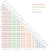 |
Fig. C.1. Same as in Fig. 7, but the full posterior PDF. |
| In the text | |
Current usage metrics show cumulative count of Article Views (full-text article views including HTML views, PDF and ePub downloads, according to the available data) and Abstracts Views on Vision4Press platform.
Data correspond to usage on the plateform after 2015. The current usage metrics is available 48-96 hours after online publication and is updated daily on week days.
Initial download of the metrics may take a while.