| Issue |
A&A
Volume 645, January 2021
|
|
|---|---|---|
| Article Number | A86 | |
| Number of page(s) | 6 | |
| Section | Astrophysical processes | |
| DOI | https://doi.org/10.1051/0004-6361/202039666 | |
| Published online | 18 January 2021 | |
Properties of a hypothetical cold pulsar wind in LS 5039
Departament de Física Quàntica i Astrofísica, Institut de Ciències del Cosmos (ICC), Universitat de Barcelona (IEEC-UB), Martí i Franquès 1, 08028 Barcelona, Spain
e-mail: vbosch@fqa.ub.edu
Received:
13
October
2020
Accepted:
14
December
2020
Context. LS 5039 is a powerful high-mass gamma-ray binary that probably hosts a young non-accreting pulsar. However, despite the wealth of data available, the means by which the non-thermal emitter is powered are still unknown.
Aims. We use a dynamical-radiative numerical model, and multiwavelength data, to constrain the properties of a hypothetical pulsar wind that would power the non-thermal emitter in LS 5039.
Methods. We ran simulations of an ultrarelativistic (weakly magnetized) cold e±-wind that Compton scatters stellar photons and that dynamically interacts with the stellar wind. The effects of energy losses on the unshocked e±-wind dynamics, and the geometry of the two-wind contact discontinuity, are computed for different wind models. The predicted unshocked e±-wind radiation at periastron, when expected to be the highest, is compared to LS 5039 data.
Results. The minimum possible radiation from an isotropic cold e±-wind overpredicts the X-ray to gamma-ray fluxes at periastron by a factor of ∼3. In the anisotropic (axisymmetric) wind case X-ray and ≳100 MeV data are not violated by wind radiation if the wind axis is at ≲20−40° from the line of sight (chance probability of ≲6−24%), depending on the anisotropic wind model, or if the wind Lorentz factor ∈102 − 103, in which case the wind power can be higher, but it requires e±-multiplicities of ∼106 and 109 for a 10−2 s and 10 s pulsar period, respectively.
Conclusions. The studied model predicts that a weakly magnetized cold pulsar e±-wind in LS 5039 should be strongly anisotropic, with either a wind Lorentz factor ∈102 − 103 and very high multiplicities or with a fine-tuned wind orientation. A weakly magnetized, cold baryon-dominated wind would be a possible alternative, but then the multiplicities should be rather low, while the baryon-to-e± energy transfer should be very efficient at wind termination. A strongly magnetized cold wind seems to be the most favorable option as it is consistent with recent research on pulsar winds and does not require fine-tuning of the pulsar wind orientation, and the wind multiplicity and Lorentz factor are less constrained.
Key words: gamma rays: stars / radiation mechanisms: non-thermal / stars: winds, outflows / stars: individual: LS 5039
© ESO 2021
1. Introduction
LS 5039 is a strong galactic source of variable and periodic gamma rays (Paredes et al. 2000; Aharonian et al. 2005a; Abdo et al. 2009; Hadasch et al. 2012; Collmar & Zhang 2014; Chang et al. 2016). This source displays non-thermal radio emission with milliarcsecond to subarcsecond components (Paredes et al. 2000, 2002) and X-rays of likely non-thermal origin (see, e.g., Bosch-Ramon et al. 2007), presenting orbital changes in morphology (Ribó et al. 2008; Moldón et al. 2012a) and flux (see, e.g., Bosch-Ramon et al. 2005; Takahashi et al. 2009), respectively. The source is a compact binary with period P ≈ 3.91 d, semi-major axis a ≈ 2.1 × 1012 cm, and eccentricity e ≈ 0.35, and hosts a O6.5V star and an undetermined compact object (CO) of a few solar masses (Casares et al. 2005). The source was initially thought to be a radio-loud X-ray binary (Marti et al. 1998), and a gamma-ray emitting microquasar later on (Paredes et al. 2000). The proposed microquasar nature and gamma-ray association led to the development of microquasar jet models for the non-thermal emitter (e.g., Paredes et al. 2000, 2006; Bosch-Ramon & Paredes 2004; Bednarek 2006; Dermer & Böttcher 2006; Khangulyan et al. 2008), although the lack of accretion signatures in X-rays, among other source features, and the gamma-ray detection of PSR B1259−63/LS2883 (Aharonian et al. 2005b, a similar source hosting a non-accreting pulsar), led to the suggestion that LS 5039 hosted a young non-accreting pulsar (Martocchia et al. 2005; Dubus 2006a).
Orbital radial-velocity measurements have not yet determined the LS 5039 CO mass (Casares et al. 2005; Sarty et al. 2011). Several works have studied the structure of its non-thermal emitter using modeling and/or radio (Ribó et al. 2008; Bosch-Ramon 2009; Moldón et al. 2012a), ultraviolet (Szostek et al. 2012), X-ray (Bosch-Ramon et al. 2007; Bosch-Ramon 2010; Szostek & Dubus 2011; Zabalza et al. 2011), and gamma-ray data (e.g., Bosch-Ramon et al. 2008a; Khangulyan et al. 2008; Cerutti et al. 2010; Zabalza et al. 2013; Dubus et al. 2015), as well as hydrodynamical simulations (Perucho et al. 2010; Bosch-Ramon et al. 2015). These studies show, for instance, that the emitter is likely extended and/or relatively far from the CO, but they could not clearly favor any particular scenario.
Recently, Yoneda et al. (2020) have presented evidence of X-ray pulsations in LS 5039. Despite the relatively low statistical significance of the detection, and an unexpectedly long period of ≈9 s, these results add significant weight to the pulsar scenario. As the pulsation period is rather long, Yoneda et al. (2020) suggest that the neutron star is in fact a magnetar, although the very young age estimated for the CO, ∼500 yr, seems to be at odds with the lack of evidence of the presence of a supernova remnant (SNR; Moldón et al. 2012b). We note that finding a much shorter period was not possible for Yoneda et al. (2020) as the data statistics only allowed the search of periods > 1 s.
Regardless of the specific pulsar nature, if a pulsar wind transports the energy from the CO to the non-thermal emitter, the wind can radiate much of its energy even before being shocked by the stellar wind. In particular, inverse Compton (IC) scattering off stellar photons by an ultrarelativistic cold pulsar e±-wind (Bogovalov & Aharonian 2000) is very efficient in a compact binary (see, e.g., Ball & Kirk 2000; Sierpowska & Bednarek 2005; Khangulyan et al. 2007; Sierpowska-Bartosik & Torres 2007; Cerutti et al. 2008; Khangulyan et al. 2011; Hu et al. 2020), and in LS 5039 the expected IC fluxes may be higher than the observed ones (Cerutti et al. 2008). The total non-thermal luminosity of LS 5039 is consistently high all along the orbit, at a level LNT ≈ 1036 erg s−1 (mostly released in the MeV-GeV range, Abdo et al. 2009; Collmar & Zhang 2014; at 2.1 kpc, Gaia Collaboration 2018; Luri et al. 2018), which is hardly compatible with Doppler boosting (Db) models (see below), meaning that the pulsar wind luminosity Lp must indeed be > LNT.
In this work we revisit the (weakly magnetized) cold pulsar e±-wind model in the context of LS 5039 to constrain the hypothetical wind properties, using for the first time the most recent data in X-rays and soft and hard gamma rays. We model how such a wind transports the energy from the pulsar to its termination shock, which is produced by the interaction with the stellar wind. Unlike previous works, to compute the geometry of the stellar-pulsar wind interaction region we include the pulsar wind momentum-flux losses and orbital motion. As in Cerutti et al. (2008), we consider both isotropic and anisotropic wind models, and assume that the e±-wind does not heat up due to IC braking. In Sects. 2 and 3 we present our wind model and its results, respectively, adopting parameter values that minimize the e±-wind IC emission at periastron, the orbital phase when this emission should be the brightest (i.e., the most constraining choice). We conclude and discuss the results in Sect. 4.
2. Model
The cold pulsar e±-wind propagation, radiation, and termination location were computed including the orbit effect on the geometry of the contact discontinuity (CD) between the pulsar and the stellar wind. A description of the model and the approach adopted for these calculations are presented in what follows.
To derive the most stringent constraints on the wind radiation towards the observer, we focused on periastron, when this radiation is expected to be highest (see Cerutti et al. 2008; LS 5039 periastron orbital phase, ϕ = 0, is close to superior conjunction of the CO, ϕ ≈ 0.058, see Casares et al. 2005). At the same time, we were interested in a parameter choice predicting the minimum possible IC emission for that orbital phase. Thus, regarding the inclination, a value of i ≈ 45° was chosen, which also avoids black hole masses for the CO or stellar eclipse (Casares et al. 2005). Moreover, we fixed Lp = 2 × 1036 erg s−1, which is Lp ≈ 2LNT; in other words, the non-thermal emitter must emit ≈50% of the available power. As LNT ∼ 1036 erg s−1 all through the orbit, Db cannot be behind the high (but then apparent) LNT unless the emitting flow is always roughly pointing to the observer, which is implausible in a colliding wind system (although Db can still significantly affect the lightcurve; see, e.g., Zabalza et al. 2013; Dubus et al. 2015; Molina & Bosch-Ramon 2020). For comparison, the luminosities injected in the emitting e± of the shocked wind in Zabalza et al. (2013), Dubus et al. (2015), and Molina & Bosch-Ramon (2020), which must be < Lp, were Lrel−e = 4 × 1035, 1035, and 6 × 1035 erg s−1, respectively. All three works accounted for Db in the shocked-wind emitter, and the last two severely underpredicted the flux in MeV (not considered by Zabalza et al. 2013).
We computed for all directions the energy evolution of the wind e±, which moved from the CO along straight trajectories as they IC scattered stellar photons. We used an iterative scheme to follow the e± energy, with IC energy losses and emission determined by IC interactions in the anisotropic blackbody stellar field (Khangulyan et al. 2014). Descriptions of how to calculate the e± propagation, energy loss, and emission can be found in Cerutti et al. (2008) and Khangulyan et al. (2011), among others. For simplicity, a point-like star was considered when computing the IC emission in different directions, which is reasonable as i is such that gamma rays are not eclipsed. When computing the anisotropic IC losses for all directions the interaction angle was set to be at least the angle subtended by the star and at most its supplementary, as seen from the emitting point, accounting in this way for the actual star finite size.
The wind magnetic field (B) was taken to be irrelevant both dynamically and, as a cold e± wind does not produce synchrotron radiation, radiatively. The explored initial Lorentz factors of the wind were Γp, 0 ∈ 10−105. Gamma-ray absorption and reprocessing were not included in the calculations because Γp, 0 ≫ 105 is needed for efficient pair creation and cascading in the stellar photon field. Not accounting for such a high Γp, 0 is reasonable as in LS 5039 the reprocessed gamma-ray luminosity of an e±-wind should be still a significant fraction of Lp, peaking around multi-GeV energies (see Sierpowska & Bednarek 2005, for a similar system), which is at odds with the rather low flux of LS 5039 at ∼10 GeV (see the overall gamma-ray spectrum in, e.g., Hadasch et al. 2012; Collmar & Zhang 2014). Not accounting for gamma-ray reprocessing simplifies the calculations greatly as otherwise one would need a detailed knowledge of the background medium (for these process complexities in LS 5049, see, e.g., Aharonian et al. 2006; Dubus 2006b; Bednarek 2006; Sierpowska-Bartosik & Torres 2007; Khangulyan et al. 2008; Bosch-Ramon et al. 2008b,a; Cerutti et al. 2010; Bosch-Ramon & Khangulyan 2011).
The IC braking effect on Γp was computed for all the possible trajectories up to three times the orbital separation (i.e., 3 × Rorb), and the shape of the two-wind CD was calculated including the orbit effect. Five approximations were adopted for the initial e±-energy and for the energy and momentum flux angular dependence: (case A) an isotropic e±-wind; (cases B and B′) a phenomenological axisymmetric e±-wind with constant Γp, 0 and
for B and
for B′, being θp the angle with the pulsar wind symmetry axis; and (cases C and C′) a more physical axisymmetric wind with

for C and

for C′ (see, e.g., Cerutti et al. 2008; Tchekhovskoy et al. 2016, and Bogovalov & Khangoulyan 2002 in the context of Crab). The explored values for  were ∈10−105 (as they were for Γp, 0). The line-of-sight angle of the e±-wind axis in cases B and C was set to ψ = 20°, and in cases B′ and C′ to ψ = 40°, not to violate the observed fluxes. Several e±-wind orientations were tested fulfilling ψ ≈ 20° and 40°, and to be conservative we chose those with the lowest IC fluxes. The probability of having a smaller ψ-value was P ≲ 6% for cases B and C, and P ≲ 24% for cases B′ and C′. The stellar wind was assumed to be spherically symmetric, although a prescription for its momentum flux ∝sin2θw was also tested, with the plane defined by θw = π/2 passing through the pulsar center (the most conservative case); both prescriptions yielded very similar results.
The stellar wind was assumed to be cold, with momentum flux of
and velocity of

in the non-inertial frame rotating with the orbit angular velocity (Ω), where θ is the angle to the orbit normal, R* the stellar radius, and d the stellar distance. To normalize ṗw, the maximum possible mass-loss rate for this wind, Ṁ = 7 × 10⁻⁷ M⊙ yr−1, was adopted (Casares et al. 2005), minimizing the distance covered by the unshocked e±-wind, and thus its IC emission. Nevertheless, the Ṁ-dependence of the e±-wind IC luminosity is weak, as the pulsar wind facing the observer at periastron typically loses most of its energy (see below). The stellar wind velocity at infinity v∞ was fixed to 2.44 × 108 cm s −1, and β to 1, while the minimum radial velocity was set to the escape velocity, ≈108 cm s −1 (McSwain et al. 2004).
The e±-wind, little affected by Coriolis forces due to its high speed, was assumed with zero pressure, radial from the pulsar, and with momentum flux of
and velocity of
The e±-wind anisotropy was introduced via ρp (B and B′) and Γp, 0 (C and C′). Losses affected Γp.
The CD was computed using an approach based on the thin shell axisymmetric approximation (see, e.g., Antokhin et al. 2004 for a radiative shell; also approximately valid for a thicker, adiabatic hydrodynamic shell), but modified to account for the lack of axisymmetry due to the orbit-related Coriolis force and the wind anisotropy.
First, the CD stagnation point (SP), at which

is found. We looked for the SP assuming that it was on the orbital plane, in a direction from the pulsar tilted from the pulsar-star direction clockwise by an angle
where ωorb is the orbit angular velocity and η = (Lp/Ṁ|vw|c) is the momentum rate ratio of the pulsar and the stellar wind. This approximation works well for small τ, so we adopted this method in our calculations as a first-order approximation. Once found, we took the SP position as the initial one and computed the paths shaping the CD in all directions through an iterative process. The iterative steps in each path provide segments that characterize the CD surface step by step. To find the directions of the new segments, we used the relations
and
at each step, where αw and αp are the complementary angles between the stellar and the pulsar wind directions and the CD normal, respectively, and ṗs is the momentum flux remaining after wind collision, at the segment location on the CD. The thin shell approximation allows the cancellation of the opposing momentum components. Once a direction on the CD surface from the SP is chosen, the next point is defined by the local direction of ṗs and a sufficiently small distance in that direction. Even if αw and αp are not known, the direction of ṗs can be computed by eliminating one of the α parameters using Eq. (11), and renormalizing ṗs to eliminate the other one from Eq. (12).
To account for the shocked region of the e±-wind between the termination shock and the CD, the e±-wind was terminated at ≈2/3 of the distance from the pulsar to the CD (see Bogovalov et al. 2008 for cases with η ≲ 0.01, although if B were strong it would largely modify the overall interaction structure, see Bogovalov et al. 2019). In the presence of orbital motion, analytical and numerical calculations show that a strong shock should terminate the pulsar wind due to Coriolis forces in the directions away from the star (see, e.g., Bosch-Ramon & Barkov 2011; Bosch-Ramon et al. 2012, 2015; Huber et al. 2020). Therefore, the unshocked pulsar wind, and the CD itself, were simply assumed to stop in these directions at the distance where such a Coriolis shock is expected to form. Since we focus on periastron, our results are not affected by this assumption as the relevant line of sight does cross the computed CD at that phase.
3. Results
The cold pulsar e±-wind IC fluxes were computed for cases A, B and B′, and C and C′. The pulsar orientation in B and C, and in B′ and C′, was chosen such that ψ ≈ 20° (P ≲ 6%) and 40° (P ≲ 24%), respectively. The remaining parameter values were as follows: R* = 10 R⊙; effective stellar temperature T = 4 × 10⁴ K; e = 0.35; P = 3.91 d; ϕ = 0 (Rorb ≈ 1.4 × 1012 cm); i = 45°; Ṁ = 7 × 10⁻⁷ M⊙ yr−1; v∞ = 2.44 × 108 cm s −1 and β = 1; Lp = 2 × 1036 erg s−1; and Γp, 0 ∈ 10−105.
The paths characterizing the CD surface for case A are shown in the top panel of Fig. 1 for Γp, 0 = 10 and 105, with and without orbital motion (the CD shapes for B and C, and B′ and C′ were very similar, although a detailed discussion is beyond the scope of this work). The CD shrinks by a factor of ∼2 due to stronger IC losses for Γp, 0 = 105, as the cooling time is  in the explored range. Orbital motion clearly affects the CD geometry on the scales of the orbital separation for the parameter values adopted, although the computed e±-wind IC fluxes without orbital motion (see the dashed line in the top panel of Fig. 1) were almost the same. The bottom panel of Fig. 1 shows two maps of the fraction of the energy remaining in the e± after IC losses for case A, with Γp, 0 = 10 (right) and 105 (left), together with the corresponding orbital-plane CD shapes. As expected, for Γp, 0 = 10 e± lose ∼1% of their energy or less when reaching the CD, whereas for Γp, 0 = 105 they lose ∼80% towards the star, and ∼20% away from it.
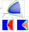 |
Fig. 1. Top panel: orbital plane projection of the computed paths on the CD surface, at periastron, for case A and Γp, 0 = 10 (green; more extended) and 105 (blue; more compact), including orbital motion. The red dashed line shows the profile of the structure for Γp, 0 = 105 when orbital motion is not included. The projected line of sight points along |

The e±-wind spectral energy distributions are shown in Fig. 2 for Γp, 0 ∈ 10−105, and for cases A, B, and C. The spectral energy distributions for cases B′ and C′ (not shown) are very similar to those of B and C, as expected given that the ψ-value choice is determined by the same observational constraints. An isotropic e±-wind (A) overpredicts the observed fluxes by at least a factor of ≈3. The anisotropic e±-wind of cases B and C, with ψ ≲ 20° between the wind symmetry axis and the line of sight, does not overpredict the observed X-ray or ≳100 MeV fluxes if Γp, 0 ∉ 102 − 103. The IC flux of cases B and C is also lower than the observed ∼0.1−30 MeV fluxes by a factor of ≈3−5 for Γp, 0 ∈ 102 − 103, which allows the relaxation of the constraint on ψ from ≲20° to ≲45° (P ≲ 30%) for Lp ≳ 2 × 1036 erg s−1. In the anisotropic e±-wind model of cases B′ and C′, the observed X-ray and ≳100 MeV fluxes constrain ψ to ≲40° (P ≲ 24%) if Γp, 0 ∉ 102 − 103. On the other hand, the observed ∼0.1−30 MeV fluxes do not constrain ψ at all in cases B′ and C′ for Γp, 0 ∈ 102 − 103 if Lp ≳ 2 × 1036 erg s−1. The X-ray data, having high statistics, constrains a narrow spectral component to a level of a ∼10% of the observed fluxes (see, e.g., Bosch-Ramon et al. 2007). Thus, Cases B and B′ are also constrained by X-ray data even though the predicted flux is ∼3 times lower than observed.
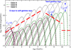 |
Fig. 2. Computed spectral energy distributions of the IC cold pulsar wind emission, at periastron, for 11 different Γp, 0 values from Γp, 0 = 10 to 105, for cases A (dotted lines), B (dashed lines), and C (solid lines) (cases B′ and C′ are very similar; see main text). A schematic spectral energy distribution based on the observed X-ray to gamma-ray emission around superior conjunction (adapted from Fig. 9 in Collmar & Zhang 2014; see references therein), which is close to periastron, is also shown. |
4. Conclusions and discussion
4.1. Weakly magnetized cold wind model
If LS 5039 has a weakly magnetized cold pulsar e±-wind carrying the energy to the non-thermal emitter, this wind cannot be isotropic as this is inconsistent with observations, even for ratios of the total broadband non-thermal radiation luminosity to the pulsar wind power of LNT/Lp ∼ 1.
An anisotropic wind with angular dependence ∝sin2θp does not violate the observational constraints, but requires either a very high LNT/Lp ∼ 1, even for the most favorable Γp, 0 values, or an unlikely orientation. For cases B and C and Γp, 0 ∉ 102 − 103, even for an unrealistic LNT/Lp ≈ 0.5 a rather improbable ψ ≲ 20° (P ≲ 6%) is required for the predictions to be consistent with X-ray and gamma-ray data. For the same cases but where Γp, 0 ∈ 102 − 103, ψ is less constrained, ≲45° (P ≲ 30%), if LNT/Lp ≈ 0.5 is kept. Smaller ψ-values relax the energetic constraints when Γp, 0 ∈ 102 − 103, but reduce the associated probability: for LNT/Lp ≈ 0.1, ψ ≲ 20° and thus P ≲ 6%. We note that LNT/Lp ≈ 0.1 is still quite high, typically values of Lrel−e/Lp ∼ 0.1 are adopted in the modeling of the whole LS 5039 non-thermal emission, resulting in an even lower LNT/Lp value. We recall that invoking Db can reduce the energetic requirements in some orbital phases, but not everywhere in the orbit.
If the wind is even more anisotropic, with angular dependence ∝sin4θp, the situation becomes less dramatic, although quite high LNT/Lp values are still needed in general. For cases B′ and C′ and Γp, 0 ∉ 102 − 103, setting LNT/Lp ≈ 0.5 implies that ψ ≲ 40° (P ≲ 24%) does not violate the observed fluxes, whereas for Γp, 0 ∈ 102 − 103 the angle ψ is not constrained at all. Adopting ψ-values significantly smaller than ≈40°, LNT/Lp becomes virtually unconstrained for Γp, 0 ∈ 10−105 in B′, and for Γp, 0 ∈ 102 − 105 in case C′ (in C′ taking Γp, 0 ≲ 102 still overpredicts the X-ray fluxes). Therefore, in cases B′ and C′ the data are less restrictive than B and C of the e±-wind properties, but some fine-tuning in ψ or Γp, 0 is still needed if a high LNT/Lp is to be avoided.
Despite all this discussion on wind anisotropy, it is worth noting that fine-tuning the wind orientation is less effective in relaxing the energetic requirements on Lp if the pulsar precesses (Stairs et al. 2000). In addition, the wind anisotropy is likely to be more complex than just described (see, e.g., Philippov & Spitkovsky 2018), which can smear its effects and thus make wind orientation fine-tuning less effective in relaxing the observational constraints.
To explore the e±-multiplicity κ in the studied wind model, one can take for instance Γp, 0 = 3 × 10² and Lp ∼ 1037 erg s−1, values allowed by observations for ψ ≲ 20° in B and C, and in a broader range of ψ-values in B′ and C′. With this choice of parameters, κ should be ∼106 (∼109) for a 10 km radius pulsar with 1012 G (1015 G) surface B and 10−2 s (10 s) period.
A weakly magnetized cold baryonic wind is an alternative to a pure e±-wind model. Such a wind would require that baryons reach Γp, 0 ≳ 5 × 10⁴ (≳5 × 10⁷–10 s-) for Lp ≳ 2 × 1036 erg s−1, while κ ≲ 10 (≲104–10 s-), so as not to violate the ≳10 GeV (≳1 TeV -10 s-) fluxes for an isotropic wind, and ≲102 (≲105–10 s-) for an anisotropic wind with ψ ≈ 20° (B and C) or ≈40° (B′ and C′). We note that this scenario requires very efficient proton-to-e± transfer at wind termination, as multiplicity limits become tighter for higher proton wind luminosity budgets. We consider here protons solely for energy transport as a non-thermal proton emitter in LS 5039 is likely to be radiatively inefficient due to not enough ambient photon energy, and radiation and wind densities (Bosch-Ramon & Khangulyan 2009).
4.2. Magnetized winds
A strongly magnetized flow produced by a young magnetar in LS 5039 was proposed by Yoneda et al. (2020) prompted by the evidence of a ≈9 s period in X-ray data. As indicated in Sect. 1, the young magnetar hypothesis put forward in that work is at odds with the lack of evidence for a SNR, and the physics of such a flow would be more uncertain than that of more standard pulsar wind models. Interestingly, it is also possibile to envision an exotic explanation for the ≈9 s period unrelated to pulsar rotation. LS 5039 might instead host not one CO, but an extremely close CO binary of semi-major axis ≈109 cm. Such a binary, given the mass function of the system (Casares et al. 2005), would most likely be formed by two neutron stars. The neutron stars might have rotation periods much shorter than ≈9 s, for instance in the millisecond range. Now, whether such a configuration is plausible from the point of view of stellar evolution is to be studied elsewhere (see, e.g., Abbott et al. 2020, in the context of gravitational wave detections of related systems).
Nevertheless, for the single-CO scenario a pulsar wind with a dynamically significant magnetic field would be in agreement with recent research on pulsar winds, which proposes average magnetization parameters σ ∼ 1 instead of ∼10−2 − 10−3 (Amato 2020), where

with ṁ being the wind mass rate. Unfortunately, the complexity of a magnetized wind (as exemplified for instance in the simulations by Philippov & Spitkovsky 2018) does not allow the use of a simple, but still physically consistent, prescription for the wind like the one employed here for the cold, matter-dominated case. However, we can already show that a strongly magnetized wind may be, given the observational constraints, the most favored scenario in LS 5039:
As in the case of a cold baryonic wind, a magnetized wind would not produce prominent narrow X-ray and gamma-ray spectral features if the wind e± did not get energized by B-dissipation until wind termination (and e±-energy redistribution). However, for a strongly magnetized wind, the constraints on κ and Γp, 0 are looser than in the baryonic wind case, as now Γp, 0 is also not constrained. For Γp, 0 ≲ 104, we obtain κΓp, 0 ≲ 107 (≲1010 -10 s-) for case A, implying σ ≳ 10. For Γp, 0 ≳ 104, σ must be higher due to tighter observational constraints above the GeV range. For cases B, C, B′, and C′ the observational constraints on a weakly magnetized wind are looser for specific orientations, and thus less demanding on sigma, but high sigma values render wind orientation fine-tuning (which has its caveats, as already mentioned) unnecessary. Therefore, we conclude that a high-sigma wind is less constrained and thus seems more favorable than the other two scenarios.
4.3. Hot winds
It is possible that, relatively early in its propagation, the pulsar wind turns a significant amount of energy (magnetic or kinetic) into non-thermal energy, meaning that the non-thermal emitter would start much closer to the pulsar than the wind termination shock (see, e.g., Sierpowska-Bartosik & Torres 2007; Pétri & Dubus 2011; Derishev et al. 2012, for the presence of non-thermal particles in the wind of LS 5039 due, e.g., to magnetic dissipation, IC cascades). This scenario is perhaps the hardest to model, and may not be consistent with evidence of fast e±-wind acceleration in the Crab pulsar (see Aharonian et al. 2012), although in a high-mass binary system the unshocked pulsar wind has a very different environment than in an isolated pulsar. On the other hand, it is worth noting that observations of LS 5039 strongly suggest that significant particle acceleration is still required far from the CO as the X-ray and particularly the very high-energy emission seem to originate in the binary outskirts (see Sect. 1). This peripheric accelerator must be very efficient as acceleration rates close to the electrodynamical limit have been inferred from the very high-energy data (see Khangulyan et al. 2008). Nevertheless, it cannot be discounted that the bulk of the ∼0.1−30 MeV emission may still be produced in a hot wind, relatively close to the pulsar (as proposed in Derishev et al. 2012, effectively similar to the cold e∓-wind case with Γp, 0 ∈ 102 − 103 discussed here)1.
4.4. Similar sources
We finish by noting that, in addition to LS 5039, four other high-mass gamma-ray binaries, LS I +61 303, 1FGL J1018.6−5856, LMC P3, and 4FGL J1405−6119, are approximately as compact and at least as powerful as LS 5039, with a relatively similar phenomenology and unknown CO (see Sect. 1 in Molina & Bosch-Ramon 2020, and references therein). Although all these sources deserve specific studies of their own, an approach such as the one presented here can be helpful to constrain the properties of a hypothetical pulsar wind powering their non-thermal emitter.
Acknowledgments
We thank the anonymous referee for constructive and useful comments that helped to improve the manuscript. We are grateful to Dmitry Khangulyan for insightful comments on this work. V.B-R. acknowledges financial support by the Spanish Ministerio de Economía, Industria y Competitividad (MINEICO/FEDER, UE) under grant AYA2016-76012-C3-1-P, from the State Agency for Research of the Spanish Ministry of Science and Innovation under grant PID2019-105510GB-C31 and through the ”Unit of Excellence María de Maeztu 2020-2023” award to the Institute of Cosmos Sciences (CEX2019-000918-M), and by the Catalan DEC grant 2017 SGR 643. V.B-R. is Correspondent Researcher of CONICET, Argentina, at the IAR.
References
- Abbott, R., Abbott, T. D., Abraham, S., et al. 2020, ApJ, 896, L44 [Google Scholar]
- Abdo, A. A., Ackermann, M., Ajello, M., et al. 2009, ApJ, 706, L56 [NASA ADS] [CrossRef] [Google Scholar]
- Aharonian, F., Akhperjanian, A. G., Aye, K. M., et al. 2005a, Science, 309, 746 [NASA ADS] [CrossRef] [PubMed] [Google Scholar]
- Aharonian, F., Akhperjanian, A. G., Aye, K. M., et al. 2005b, A&A, 442, 1 [NASA ADS] [CrossRef] [EDP Sciences] [Google Scholar]
- Aharonian, F., Anchordoqui, L., Khangulyan, D., & Montaruli, T. 2006, J. Phys. Conf. Ser., 39, 408 [NASA ADS] [CrossRef] [Google Scholar]
- Aharonian, F. A., Bogovalov, S. V., & Khangulyan, D. 2012, Nature, 482, 507 [NASA ADS] [CrossRef] [PubMed] [Google Scholar]
- Amato, E. 2020, ArXiv e-prints [arXiv:2001.04442] [Google Scholar]
- Antokhin, I. I., Owocki, S. P., & Brown, J. C. 2004, ApJ, 611, 434 [NASA ADS] [CrossRef] [Google Scholar]
- Ball, L., & Kirk, J. G. 2000, Astropart. Phys., 12, 335 [NASA ADS] [CrossRef] [Google Scholar]
- Bednarek, W. 2006, MNRAS, 368, 579 [NASA ADS] [CrossRef] [Google Scholar]
- Bogovalov, S. V., & Aharonian, F. A. 2000, MNRAS, 313, 504 [NASA ADS] [CrossRef] [Google Scholar]
- Bogovalov, S. V., & Khangoulyan, D. V. 2002, Astron. Lett., 28, 373 [NASA ADS] [CrossRef] [Google Scholar]
- Bogovalov, S. V., Khangulyan, D. V., Koldoba, A. V., Ustyugova, G. V., & Aharonian, F. A. 2008, MNRAS, 387, 63 [Google Scholar]
- Bogovalov, S. V., Khangulyan, D., Koldoba, A., Ustyugova, G. V., & Aharonian, F. 2019, MNRAS, 490, 3601 [CrossRef] [Google Scholar]
- Bosch-Ramon, V. 2009, A&A, 493, 829 [NASA ADS] [CrossRef] [EDP Sciences] [Google Scholar]
- Bosch-Ramon, V. 2010, in High Energy Phenomena in Massive Stars, eds. J. Martí, P. L. Luque-Escamilla, & J. A. Combi, ASP Conf. Ser., 422, 77 [Google Scholar]
- Bosch-Ramon, V., & Barkov, M. V. 2011, A&A, 535, A20 [NASA ADS] [CrossRef] [EDP Sciences] [Google Scholar]
- Bosch-Ramon, V., & Khangulyan, D. 2009, Int. J. Mod. Phys. D, 18, 347 [Google Scholar]
- Bosch-Ramon, V., & Khangulyan, D. 2011, PASJ, 63, 1023 [NASA ADS] [Google Scholar]
- Bosch-Ramon, V., & Paredes, J. M. 2004, A&A, 417, 1075 [NASA ADS] [CrossRef] [EDP Sciences] [Google Scholar]
- Bosch-Ramon, V., Paredes, J. M., Ribó, M., et al. 2005, ApJ, 628, 388 [NASA ADS] [CrossRef] [Google Scholar]
- Bosch-Ramon, V., Motch, C., Ribó, M., et al. 2007, A&A, 473, 545 [NASA ADS] [CrossRef] [EDP Sciences] [Google Scholar]
- Bosch-Ramon, V., Khangulyan, D., & Aharonian, F. A. 2008a, A&A, 489, L21 [NASA ADS] [CrossRef] [EDP Sciences] [Google Scholar]
- Bosch-Ramon, V., Khangulyan, D., & Aharonian, F. A. 2008b, A&A, 482, 397 [Google Scholar]
- Bosch-Ramon, V., Barkov, M. V., Khangulyan, D., & Perucho, M. 2012, A&A, 544, A59 [NASA ADS] [CrossRef] [EDP Sciences] [Google Scholar]
- Bosch-Ramon, V., Barkov, M. V., & Perucho, M. 2015, A&A, 577, A89 [NASA ADS] [CrossRef] [EDP Sciences] [Google Scholar]
- Casares, J., Ribó, M., Ribas, I., et al. 2005, MNRAS, 364, 899 [Google Scholar]
- Cerutti, B., Dubus, G., & Henri, G. 2008, A&A, 488, 37 [NASA ADS] [CrossRef] [EDP Sciences] [Google Scholar]
- Cerutti, B., Malzac, J., Dubus, G., & Henri, G. 2010, A&A, 519, A81 [NASA ADS] [CrossRef] [EDP Sciences] [Google Scholar]
- Chang, Z., Zhang, S., Ji, L., et al. 2016, MNRAS, 463, 495 [NASA ADS] [CrossRef] [Google Scholar]
- Collmar, W., & Zhang, S. 2014, A&A, 565, A38 [NASA ADS] [CrossRef] [EDP Sciences] [Google Scholar]
- Derishev, E. V., & Aharonian, F. A. 2012, in American Institute of Physics Conference Series, eds. F. A. Aharonian, W. Hofmann, & F. M. Rieger, Am. Inst. Phys. Conf. Ser., 1505, 402 [Google Scholar]
- Dermer, C. D., & Böttcher, M. 2006, ApJ, 643, 1081 [NASA ADS] [CrossRef] [Google Scholar]
- Dubus, G. 2006a, A&A, 456, 801 [NASA ADS] [CrossRef] [EDP Sciences] [Google Scholar]
- Dubus, G. 2006b, A&A, 451, 9 [NASA ADS] [CrossRef] [EDP Sciences] [Google Scholar]
- Dubus, G., Lamberts, A., & Fromang, S. 2015, A&A, 581, A27 [NASA ADS] [CrossRef] [EDP Sciences] [Google Scholar]
- Gaia Collaboration (Brown, A. G. A., et al.) 2018, A&A, 616, A1 [NASA ADS] [CrossRef] [EDP Sciences] [Google Scholar]
- Hadasch, D., Torres, D. F., Tanaka, T., et al. 2012, ApJ, 749, 54 [Google Scholar]
- Hu, X., Jumpei, T., & Qingwen, T. 2020, MNRAS, submitted [arXiv:2004.04337] [Google Scholar]
- Huber, D., Kissmann, R., Reimer, A., & Reimer, O. 2020, ArXiv e-prints [arXiv:2012.04975] [Google Scholar]
- Khangulyan, D., Hnatic, S., Aharonian, F., & Bogovalov, S. 2007, MNRAS, 380, 320 [Google Scholar]
- Khangulyan, D., Aharonian, F., & Bosch-Ramon, V. 2008, MNRAS, 383, 467 [NASA ADS] [CrossRef] [Google Scholar]
- Khangulyan, D., Aharonian, F. A., Bogovalov, S. V., & Ribó, M. 2011, ApJ, 742, 98 [NASA ADS] [CrossRef] [Google Scholar]
- Khangulyan, D., Aharonian, F. A., & Kelner, S. R. 2014, ApJ, 783, 100 [NASA ADS] [CrossRef] [Google Scholar]
- Luri, X., Brown, A. G. A., Sarro, L. M., et al. 2018, A&A, 616, A9 [NASA ADS] [CrossRef] [EDP Sciences] [Google Scholar]
- Marti, J., Paredes, J. M., & Ribo, M. 1998, A&A, 338, L71 [Google Scholar]
- Martocchia, A., Motch, C., & Negueruela, I. 2005, A&A, 430, 245 [NASA ADS] [CrossRef] [EDP Sciences] [Google Scholar]
- McSwain, M. V., Gies, D. R., Huang, W., et al. 2004, ApJ, 600, 927 [NASA ADS] [CrossRef] [Google Scholar]
- Moldón, J., Ribó, M., & Paredes, J. M. 2012a, A&A, 548, A103 [NASA ADS] [CrossRef] [EDP Sciences] [Google Scholar]
- Moldón, J., Ribó, M., Paredes, J. M., et al. 2012b, A&A, 543, A26 [NASA ADS] [CrossRef] [EDP Sciences] [Google Scholar]
- Molina, E., & Bosch-Ramon, V. 2020, A&A, 641, A84 [CrossRef] [EDP Sciences] [Google Scholar]
- Paredes, J. M., Martí, J., Ribó, M., & Massi, M. 2000, Science, 288, 2340 [Google Scholar]
- Paredes, J. M., Ribó, M., Ros, E., Martí, J., & Massi, M. 2002, A&A, 393, L99 [NASA ADS] [CrossRef] [EDP Sciences] [Google Scholar]
- Paredes, J. M., Bosch-Ramon, V., & Romero, G. E. 2006, A&A, 451, 259 [NASA ADS] [CrossRef] [EDP Sciences] [Google Scholar]
- Perucho, M., Bosch-Ramon, V., & Khangulyan, D. 2010, A&A, 512, L4 [NASA ADS] [CrossRef] [EDP Sciences] [Google Scholar]
- Pétri, J., & Dubus, G. 2011, MNRAS, 417, 532 [NASA ADS] [CrossRef] [Google Scholar]
- Philippov, A. A., & Spitkovsky, A. 2018, ApJ, 855, 94 [NASA ADS] [CrossRef] [Google Scholar]
- Ribó, M., Paredes, J. M., Moldón, J., Martí, J., & Massi, M. 2008, A&A, 481, 17 [NASA ADS] [CrossRef] [EDP Sciences] [Google Scholar]
- Sarty, G. E., Szalai, T., Kiss, L. L., et al. 2011, MNRAS, 411, 1293 [Google Scholar]
- Sierpowska, A., & Bednarek, W. 2005, MNRAS, 356, 711 [NASA ADS] [CrossRef] [Google Scholar]
- Sierpowska-Bartosik, A., & Torres, D. F. 2007, ApJ, 671, L145 [Google Scholar]
- Stairs, I. H., Lyne, A. G., & Shemar, S. L. 2000, Nature, 406, 484 [NASA ADS] [CrossRef] [Google Scholar]
- Szostek, A., & Dubus, G. 2011, MNRAS, 411, 193 [Google Scholar]
- Szostek, A., Dubus, G., & McSwain, M. V. 2012, MNRAS, 420, 3521 [CrossRef] [Google Scholar]
- Takahashi, T., Kishishita, T., Uchiyama, Y., et al. 2009, ApJ, 697, 592 [Google Scholar]
- Tchekhovskoy, A., Philippov, A., & Spitkovsky, A. 2016, MNRAS, 457, 3384 [NASA ADS] [CrossRef] [Google Scholar]
- Yoneda, H., Makishima, K., Enoto, T., et al. 2020, Phys. Rev. Lett., 125, 111103 [CrossRef] [Google Scholar]
- Zabalza, V., Bosch-Ramon, V., & Paredes, J. M. 2011, ApJ, 743, 7 [Google Scholar]
- Zabalza, V., Bosch-Ramon, V., Aharonian, F., & Khangulyan, D. 2013, A&A, 551, A17 [NASA ADS] [CrossRef] [EDP Sciences] [Google Scholar]
All Figures
|
Fig. 1. Top panel: orbital plane projection of the computed paths on the CD surface, at periastron, for case A and Γp, 0 = 10 (green; more extended) and 105 (blue; more compact), including orbital motion. The red dashed line shows the profile of the structure for Γp, 0 = 105 when orbital motion is not included. The projected line of sight points along |
| In the text | |
|
Fig. 2. Computed spectral energy distributions of the IC cold pulsar wind emission, at periastron, for 11 different Γp, 0 values from Γp, 0 = 10 to 105, for cases A (dotted lines), B (dashed lines), and C (solid lines) (cases B′ and C′ are very similar; see main text). A schematic spectral energy distribution based on the observed X-ray to gamma-ray emission around superior conjunction (adapted from Fig. 9 in Collmar & Zhang 2014; see references therein), which is close to periastron, is also shown. |
| In the text | |
Current usage metrics show cumulative count of Article Views (full-text article views including HTML views, PDF and ePub downloads, according to the available data) and Abstracts Views on Vision4Press platform.
Data correspond to usage on the plateform after 2015. The current usage metrics is available 48-96 hours after online publication and is updated daily on week days.
Initial download of the metrics may take a while.