| Issue |
A&A
Volume 643, November 2020
|
|
|---|---|---|
| Article Number | A7 | |
| Number of page(s) | 10 | |
| Section | Extragalactic astronomy | |
| DOI | https://doi.org/10.1051/0004-6361/202038284 | |
| Published online | 27 October 2020 | |
The ALPINE-ALMA [CII] survey
Circumgalactic medium pollution and gas mixing by tidal stripping in a merging system at z ∼ 4.57
1
Observatoire de Genève, Université de Genève, 51 Ch. des Maillettes, 1290 Versoix, Switzerland
e-mail: michele.ginolfi@unige.ch
2
Cavendish Laboratory, University of Cambridge, 19 J. J. Thomson Ave., Cambridge, CB3 0HE, UK
3
Kavli Institute for Cosmology, University of Cambridge, Madingley Road, Cambridge, CB3 0HA, UK
4
Aix Marseille Univ, CNRS, CNES, LAM, Marseille, France
5
IPAC, California Institute of Technology, 1200 East California Boulevard, Pasadena, CA, 91125, USA
6
Department of Physics, University of California, Davis, One Shields Ave., Davis, CA, 95616, USA
7
Cosmic Dawn Center (DAWN), Lyngby, Denmark
8
Niels Bohr Institute, University of Copenhagen, Lyngbyvej 2, 2100 Copenhagen, Denmark
9
Scuola Normale Superiore, Piazza dei Cavalieri 7, Pisa, 56126, Italy
10
University of Padova, Department of Physics and Astronomy, Vicolo Osservatorio 3, 35122 Padova, Italy
11
Department of Astronomy, School of Science, The University of Tokyo, 7-3-1 Hongo, Bunkyo, Tokyo, 113-0033, Japan
12
Kavli Institute for the Physics and Mathematics of the Universe, The University of Tokyo, (Kavli IPMU, WPI), Kashiwa, 277-8583, Japan
13
Caltech Optical Observatories, Cahill Center for Astronomy and Astrophysics, 1200 East California Boulevard, Pasadena, CA, 91125, USA
14
Istituto Nazionale di Astrofisica – Osservatorio di Astrofisica e Scienza dello Spazio, Via Gobetti 93/3, 40129 Bologna, Italy
15
University of Hawai’i, Institute for Astronomy, 2680 Woodlawn Drive, Honolulu, HI, 96822, USA
16
Space Telescope Science Institute, 3700 San Martin Drive, Baltimore, 21218, USA
17
University of Bologna, Department of Physics and Astronomy (DIFA), Via Gobetti 93/2, 40129 Bologna, Italy
Received:
28
April
2020
Accepted:
20
July
2020
We present ALMA observations of a merging system at z ∼ 4.57, observed as a part of the ALMA Large Program to INvestigate [CII] at Early times (ALPINE) survey. Combining ALMA [CII]158 μm and far-infrared continuum data with multi-wavelength ancillary data, we find that the system is composed of two massive (M⋆ ≳ 1010 M⊙) star-forming galaxies experiencing a major merger (stellar mass ratio rmass ≳ 0.9) at close spatial (∼13 kpc; projected) and velocity (Δv < 300 km s−1) separations, and two additional faint narrow [CII]-emitting satellites. The overall system belongs to a larger scale protocluster environment and is coincident to one of its overdensity peaks. Additionally, ALMA reveals the presence of [CII] emission arising from a circumgalactic gas structure, extending up to a diameter-scale of ∼30 kpc. Our morpho-spectral decomposition analysis shows that about 50% of the total flux resides between the individual galaxy components, in a metal-enriched gaseous envelope characterised by a disturbed morphology and complex kinematics. Similarly to observations of shock-excited [CII] emitted from tidal tails in local groups, our results can be interpreted as a possible signature of interstellar gas stripped by strong gravitational interactions, with a possible contribution from material ejected by galactic outflows and emission triggered by star formation in small faint satellites. Our findings suggest that mergers could be an efficient mechanism of gas mixing in the circumgalactic medium around high-z galaxies, and thus play a key role in the galaxy baryon cycle at early epochs.
Key words: galaxies: evolution / galaxies: formation / galaxies: high-redshift / galaxies: ISM / galaxies: interactions / intergalactic medium
© ESO 2020
1. Introduction
Modern theories of galaxy evolution and cosmological numerical simulations predict that high-z galaxies assembled their mass through a combination of cold gas accretion from the intergalactic/circumgalactic medium (IGM/CGM) and merging activity (e.g. Bower et al. 2006; Dekel et al. 2009; Hopkins et al. 2010; Vogelsberger et al. 2014; Schaye et al. 2015). Continuous baryonic flows are needed to replenish the gas content, fuel the star formation, and drive the evolution of galaxies on the star-forming main sequence (e.g. Daddi et al. 2010; Rodighiero et al. 2011; Lilly et al. 2013; Speagle et al. 2014; Scoville et al. 2016).
On the other hand, strong dynamical interactions between galaxies, such as major mergers, can efficiently drive a significant amount of gas into the central regions (e.g. Barnes & Hernquist 1991) and both (i) boost the efficiency of star formation (see Elmegreen 2000), triggering starbursts (e.g. Sanders & Mirabel 1996; Hopkins et al. 2006; Di Matteo et al. 2008; Bournaud et al. 2011), and (ii) feed the growth of super massive black holes (SMBHs), thereby powering active galactic nuclei (AGN) activity (e.g. García-Burillo et al. 2005; Di Matteo et al. 2005; Ginolfi et al. 2019). Moreover, mergers can significantly disturb and shape the morphologies of the galaxies involved, leading to the formation of tidal tails. Similarly to the ram pressure stripping (Gunn et al. 1972) extensively observed in nearby galaxy clusters (e.g. Boselli et al. 2006; Moretti et al. 2018; Poggianti et al. 2019; Fossati et al. 2019), tidal tails in merging systems are made of gas stripped from outer regions of galaxies, and extend well beyond the discs, on circumgalactic scales (e.g. Bridge et al. 2010; Wen & Zheng 2016; Guo et al. 2016; Stewart et al. 2011). As a result, strong dynamical interactions between galaxies contribute to the intergalactic transfer of processed material as shown by recent simulations (e.g. Nelson et al. 2015; Anglés-Alcázar et al. 2017; Hani et al. 2018), and, at the same time, to the chemical enrichment of the CGM (e.g. Bournaud et al. 2011; Graziani et al. 2020).
While tidal tails are well studied at different wavelengths in the local and in the intermediate redshift Universe (e.g. Poggianti et al. 2017; Vulcani et al. 2017), similar observations become challenging at higher redshift, mainly because of the diffuse and faint nature of the stripped gas. A solution comes from the Atacama Large Millimeter/sub-millimetre Array (ALMA), which enables us to possibly study the efficiency of tidal gas stripping and circumgalactic gas mixing in the early Universe, by mapping the morphology and the kinematics of the CGM around merging systems, using bright far-infrared (FIR) lines, such as [CII] 158 μm (hereafter [CII]: see Carilli & Walter 2013). In fact, [CII] has been recently detected in several star-forming galaxies at z > 4 (e.g. Capak et al. 2015; Inoue et al. 2016; Pentericci et al. 2016; Bradač et al. 2017; Carniani et al. 2018a; Matthee et al. 2019; Schaerer et al. 2020; Carniani et al. 2020), some of which are experiencing major merger events (e.g. Oteo et al. 2016; Riechers et al. 2017; Pavesi et al. 2018; Marrone et al. 2018; Decarli et al. 2019; Jones et al. 2020), or less disruptive gravitational interactions, usually revealed in combination with clumpy morphologies (e.g. Maiolino et al. 2015; Matthee et al. 2017; Jones et al. 2017; Carniani et al. 2018b). Furthermore, [CII] is generally emitted from multiple phases (ionised, neutral, and molecular gas) of the interstellar medium (ISM: e.g. Vallini et al. 2013, 2017; Lagache et al. 2018; Ferrara et al. 2019), and it has been shown to be a good tracer of shock-induced emission in the surroundings of local interacting galaxies (e.g. Cormier et al. 2012; Appleton et al. 2013; Velusamy & Langer 2014).
In this paper, we present a study of the morpho-kinematic properties of [CII] emission in and around a major merging system at z ∼ 4.57, observed as a part of the ALMA Large Program to Investigate C+ at Early Times (ALPINE) survey, that measured [CII] and FIR-continuum emission in a statistical sample of more than one-hundred normal galaxies with spectroscopic redshifts between 4 < z < 6 (see Le Fèvre et al. 2020; Béthermin et al. 2020, and Faisst et al. 2020 for descriptions of (i) the survey objectives, (ii) the ALMA data-processing, and (iii) the multi-wavelength ancillary dataset, respectively).
The paper is organised as follows. In Sect. 2, we describe the ALMA data reduction process, in Sect. 3 we report our results, and in Sect. 4 we discuss their implications. Conclusions are summarised in Sect. 5. Throughout the paper, we assume a flat ΛCDM cosmology (ΩΛ = 0.7, Ωm = 0.3, H0 = 70 km s−1 Mpc−1) and adopt a Chabrier initial mass function (IMF: Chabrier 2003). At the redshift of our target, vuds_cosmos_5101209780 (VC_9780; z[CII] = 4.573), 1 arcsec corresponds to 6.55 proper kpc.
2. ALMA observations
We conducted ALMA observations of the merging system studied in this work in Band 7 on 2 June 2018, during Cycle 5 (project 2017.1.00428.L, PI O. Le Fèvre), using a C43-2 array configuration with 45 antennae, and a total on-source time of 20 minutes. The spectral setup consisted of two sidebands, each composed of two spectral windows with total bandwidths of 1.875 GHz and channel width resolutions of 15.6 MHz. The lower sideband was tuned to the expected [CII] redshifted frequency, according to the spectroscopic redshift extracted from the rest-frame UV spectrum (drawn from the VUDS survey; Le Fèvre et al. 2015; Tasca et al. 2017). The upper sideband is used to search for FIR-continuum emission. The phase was centred at the rest-frame UV position of VC_9780 (see Sect. 3.1; RA : 10h01m33.45s; Dec : +02d22m10.19s). The data were calibrated using the automatic pipeline provided by the Common Astronomy Software Applications package (CASA; McMullin et al. 2007), version 5.4.0. No additional flagging was needed as the pipeline calibration output did not show any issues. The continuum map was obtained by running the CASA task tclean (multi-frequency synthesis mode) over the line-free visibilities in all spectral windows. The [CII] datacube was generated from the continuum-subtracted visibilities (CASA task uvcontsub), using the following setting: 500 iterations and a signal-to-noise ratio (S/N) threshold of σclean = 3 in the cleaning algorithm, a pixel size of 0.15″, and a spectral binning of 25 km s−1 (∼29 MHz). For both continuum and the [CII] datacube, we adopted a natural weighting of the visibilities to maximise the sensitivity. We reach an average root mean square (RMS) noise level at the phase centre of σcube ∼ 14 mJy beam−1 for a 25 km s−1 spectral channel in the [CII] datacube, and of σcont ∼ 60 μJy beam−1 in the continuum image. The synthesised beam in our final data products is 1.21″ × 0.77″, with a position angle of −61°. Additional information on the overall ALPINE data-processing strategy (including data quality assessment) can be found in Béthermin et al. (2020).
3. Analysis and results
3.1. A major merging system at z ∼ 4.57
Using the available ancillary data and catalogues, we first identified the system studied in this paper to be composed of two massive and rest-frame UV-bright galaxies (see an HST/ACS F814W cutout in Fig. 1a), at a mutual projected distance of ∼13 kpc: (1) VC_9780, a Lyman-break galaxy at zUV = 4.57 (confirmed z[CII] = 4.573 by ALPINE), with a stellar mass of  and a star formation rate of
  (see Faisst et al. 2020); (2) C15_7055741, at a photometric redshift zphot = 4.62 (confirmed z[CII] = 4.568, by ALPINE), with
  and
and  (from the COSMOS2015 catalogue2: Laigle et al. 2016). To simplify the reading, we dub VC_9780 and C15_705574 as #A and #B, respectively.
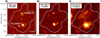 |
Fig. 1. Panel a: HST/ACS F814W (i-band; Koekemoer et al. 2007), panel b: HST/WFC3 F160W (Faisst et al., in prep.), and panel c: UltraVISTA DR4 Ks-band (McCracken et al. 2012) images of the system. The rest-frame UV positions of VC_9780 (dubbed #A) and C15_705574 (dubbed #B) are highlighted with a yellow square in panel a. The grey contour indicates the extension of the full [CII]-emitting region (see Sect. 3.3). The white bar shows a reference length of 15 kpc. North is up and east is to the left. |
For both objects, M⋆ and SFR are measured through the spectral energy distribution (SED) modelling code LePHARE (Arnouts et al. 1999; Ilbert et al. 2006; Arnouts & Ilbert 2011) run over the broadband photometry (including ground- and space-based imaging from the rest-frame UV to the near-IR; see Faisst et al. 2020) available for the well-studied COSMOS field (Scoville et al. 2007). From the HST/ACS F814W image, modelling the light profiles with a Sérsic function (Sérsic 1963) and assuming a Sérsic index n = 1 (i.e. an exponential-disc profile), we estimate rest-frame UV effective radii of re, UV = 1.0 ± 0.24 kpc and re, UV = 1.1 ± 0.3 kpc for #A and #B, respectively (see Fujimoto et al. 2020 for an accurate description of the size-fitting procedure for ALPINE galaxies).
In Fig. 1b, we show a HST/WFC3 F160W cutout of the system3 (rest-frame λrest ∼ 2800 Å), while in Fig. 1c, we display the UltraVista Ks-Band image from the fourth data release (DR44: rest-frame λrest ∼ 4000 Å), showing a faint elongation of #A towards the south east (S-E: see also Sect. 3.3). The close separation both in spatial projected distance (∼13 kpc in the HST rest-frame UV images) and redshift (|Δz| = 0.004, corresponding to an absolute velocity offset of only 270 km s−1: see Sect. 3.3) suggests that #A and #B are gravitationally bound. Moreover, the ratio of their stellar masses, rmass ∼ 0.9, is very close to unity, indicating that the galaxy system is undergoing a close major merger event (e.g. Stewart et al. 2009; Lotz et al. 2010; Jones et al. 2020).
3.2. Location at the density peak of a protocluster environment
In order to explore the larger context in which this merging event is occurring, we relied on the wealth of other spectroscopic and photometric data available in the COSMOS field to map out the large-scale galaxy density surrounding our system. The mapping was done using the Voronoi Monte Carlo (VMC) technique, first presented in Tomczak et al. (2017), Lemaux et al. (2017, 2019), and Hung et al. (2020) for use at z ∼ 1, and adapted for studies at higher redshift (2 ≤ z ≤ 5) in Cucciati et al. (2018) and Lemaux et al. (2018). This technique statistically combines both spectroscopic and photometric redshifts to generate a suite of overlapping 2D density maps in fine redshift slices over an arbitrary redshift range, and it has been shown to have high fidelity, precision, and accuracy in reconstructing the galaxy density field at a variety of different redshifts and for a variety of different observational data (see Lemaux et al. 2018 and Lemaux et al., in prep.). While we refer to the works cited above for further details, we briefly describe the method in Appendix A.
Our system is located in close projected spatial and redshift proximity to the massive proto-cluster PClJ1001 + 0220 at z ∼ 4.57, discovered by Lemaux et al. (2018). Thus, we focus here on generating a map that spans the fiducial redshift boundaries of PClJ1001 + 0220 (4.53 ≤ z ≤ 4.60). Such a redshift range corresponds to 7.5  proper kpc, or ∼3750 km s−1. As in Lemaux et al. (2018), we use the full VUDS and zCOSMOS (Lilly et al. 2007, 2009, and in prep.; Diener et al. 2013, 2015) catalogues as our primary spectroscopic catalogues, with photometric redshifts derived from fitting to the photometry presented in the COSMOS2015 catalogue (Laigle et al. 2016). In addition to the VUDS and zCOSMOS catalogues, we incorporate here new Keck II/Deep Imaging Multi-Object Spectrograph (DEIMOS, Faber et al. 2003) observations of PClJ1001 + 0220 (see a description of the observations in Lemaux et al., in prep.) which resulted in the spectroscopic confirmation of 106 new galaxies in the region in and around PClJ1001 + 0220.
Shown in Fig. 2 is the resultant VMC galaxy overdensity map for the north-east (N-E) region of the PClJ1001 + 0220 proto-cluster. Also shown are the original VUDS spectral members of the system (see Lemaux et al. 2018 for more details), as well as our #A – #B system. One of the new members confirmed by the DEIMOS observations (ID = 705080) is also shown. This galaxy, with an  and an
  , is located at ∼35
  proper kpc from our merging system, although it is not detected by ALMA, neither in [CII] nor in the rest-frame FIR continuum. Measuring its Lyα, we determine a redshift zLyα = 4.5769, corresponding to a velocity offset of Δv ∼ 260 km s−1 with respect to #A and Δv ∼ 580 km s−1 with respect to #B5. Such a close projected spatial and redshift proximity to #A – #B suggests that DEIMOS ID = 705080 is possibly associated to them.
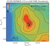 |
Fig. 2. VMC galaxy overdensity map of the N-E region of the PClJ1001 + 0220 proto-cluster (see details in Sect. 3.2). The VUDS spectral members of the system are indicated with white diamond symbols, while the location of our merging system and a possibly associated additional member observed with DEIMOS are indicated with a cyan star and a blue square, respectively. Overplotted on the map are overdensity isopleths at significance levels of [4, 6, 8, 10, 11.5, 13]σ, where σ is calculated as the RMS fluctuation of the overdensity field over the entire map (see Cucciati et al. 2018; Hung et al. 2020). The map shows that the merging system studied in this work is clearly located close to an overdensity peak of the proto-cluster. The black solid bar shows a reference length of 500 |

As can be seen in Fig. 2, our merging system at z ∼ 4.57 is nearly coincident with the overdensity peak of the N-E sub-component of the proto-cluster PClJ1001 + 0220, and lies within ≤385 pkpc of the barycentre of this sub-component. The average overdensity across this region is log(1 + ⟨δgal⟩) = 1.5, comparable to the cores of z ∼ 1 groups or the outskirts of massive clusters (e.g. Lemaux et al. 2017; Tomczak et al. 2017). All together, these findings indicate that the merging system presented in this paper belongs to a large-scale dense and complex proto-cluster environment. In Sect. 4, we discuss possible implications of this scenario in the interpretation of our results.
In the next section, we describe the results of ALMA observations of our system.
3.3. ALMA morpho-kinematics analysis
We used our ALPINE ALMA observations (see Sect. 2) of the [CII] line emission to perform a 3D morpho-spectral decomposition of our merging system. We started by extracting two spectra from large 1″ (diameter)-apertures centred on the rest-frame UV centroids of #A and #B.
We then produce velocity-integrated maps of the [CII] emission in/around #A and #B (see Fig. 3) by collapsing the cube-channels included in the spectral range [fcen − σG, fcen + σG], where fcen and σG are the central frequency and the standard deviation from a Gaussian model of the spectra. The corresponding velocity ranges are labelled in the top-left corners of both panels of Fig. 3, defined adopting a zero-velocity reference at zref = 4.570 (see next paragraphs of this section). Although this is discussed in detail later by means of tailored analyses, we note that maps in Fig. 3 already suggest a disturbed morphology of the system, showing the presence of complex resolved extended emission around the sources.
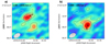 |
Fig. 3. Panel a: velocity-integrated [CII] map of VC_9780 (#A) and panel b: C15_705574 (#B), obtained by collapsing channels (velocity ranges in the upper-left corners) of line-emission in 1″-aperture spectra (see Sect. 3.3) centred on the rest-frame UV centroids of #A and #B (indicated with a black plus symbol). Black solid (dashed) contours indicate the positive (negative) significance levels at [2, 4, 8]σ of [CII] flux, where σ[CII] = 50 mJy km s−1 beam−1 in panel a and σ[CII] = 57 mJy km s−1 beam−1 in panel b. The white contours indicate the positive significance levels at [3, 4]σ of FIR-continuum emission, where σcont = 59 μJy beam−1. No negative contours at the same significance levels were found. The dashed blue ellipses indicate the beam-convolved FWHMx × FWHMy regions obtained by 2D Gaussian models, and correspond to the apertures used to extract the final [CII] spectra of #A and #B (see Sect. 3.3), shown in Fig. 4. The ALMA beam sizes are given in the bottom-left corners. North is up and east is to the left. |
We then estimated the spatial extent of the [CII]-emission arising from #A and #B by fitting a simple 2D Gaussian model to the velocity-integrated maps (Fig. 3) and used the FWHMx × FWHMy ellipses as apertures to extract the correct spectral information6.
This three-step process is needed to allow for any peculiar geometry or spatial offset between the [CII] and the rest-frame UV emission. Indeed, we note that the [CII] peak of #A is offset by ≳0.5″ from its HST centroid (see similar cases in e.g. Maiolino et al. 2015; Carniani et al. 2018a), with a clear elongation towards the S-E (see Fig. 3a). This [CII] tail is HST-dark, although a faint spike is possibly detected in the HST/WFC3 F160W image (see Fig. 1b). It is also broadly coincident with the rest-frame optical counterpart (see UltraVista DR4 Ks-band image in Fig. 1c), indicating a UV slope steeply rising towards longer wavelengths and therefore a significant presence of obscuring dust (see e.g. Calzetti et al. 2000), as also suggested by the ≳4σ ALMA detection of co-spatial FIR-continuum emission (see Fig. 3a). With the currently available ALMA resolution, it is unclear whether this [CII] tail is produced by a dust-obscured star-forming region within #A, or it is associated to a dusty neighbour at the same redshift.
The final [CII] spectra of #A and #B are shown in Fig. 4a (upper and lower panel, respectively), where we choose an intermediate redshift zref = 4.570 as a common zero-velocity reference for the system7 Galaxy #A, at ![$ z_{\mathrm{[CII]}}^{\#A} = 4.573 $](/articles/aa/full_html/2020/11/aa38284-20/aa38284-20-eq10.gif) , has a [CII]-luminosity of
, has a [CII]-luminosity of ![$ L_{\mathrm{[CII]}}^{\#A} = 3.5 ~(\pm 0.3) \times 10^8\,{L_\odot} $](/articles/aa/full_html/2020/11/aa38284-20/aa38284-20-eq11.gif) , and a FWHM#A = 190 km s−1, while #B, at
, and a FWHM#A = 190 km s−1, while #B, at ![$ z_{\mathrm{[CII]}}^{\#B} = 4.568 $](/articles/aa/full_html/2020/11/aa38284-20/aa38284-20-eq12.gif) (blueshifted by ΔvBA = −270 km s−1 with respect to #A) is broader (FWHM#B = 260 km s−1) and ∼2× more luminous,
(blueshifted by ΔvBA = −270 km s−1 with respect to #A) is broader (FWHM#B = 260 km s−1) and ∼2× more luminous, ![$ L_{\mathrm{[CII]}}^{\#B} = 6.6 ~(\pm 0.4) \times 10^8\,{L_\odot} $](/articles/aa/full_html/2020/11/aa38284-20/aa38284-20-eq13.gif) . Interestingly, the second spectrum (see lower panel of Fig. 4a) shows two additional [CII] emitters, dubbed #C and #D, spectrally offset by a few hundreds of km s−1, and spatially close to #B (less than a ∼1″-beam in projection; see velocity integrated map in the Appendix B). The line properties of #B, #C, and #D (total flux, centroid, and FWHM) are estimated from a 3-Gaussian modelling of the spectrum. Although their integrated flux is detected at > 4σ (see also Appendix B), #C and #D are very faint (
. Interestingly, the second spectrum (see lower panel of Fig. 4a) shows two additional [CII] emitters, dubbed #C and #D, spectrally offset by a few hundreds of km s−1, and spatially close to #B (less than a ∼1″-beam in projection; see velocity integrated map in the Appendix B). The line properties of #B, #C, and #D (total flux, centroid, and FWHM) are estimated from a 3-Gaussian modelling of the spectrum. Although their integrated flux is detected at > 4σ (see also Appendix B), #C and #D are very faint (![$ L_{\mathrm{[CII]}}^{\#C} = 7.7 \pm 1.5 \times 10^7\,{L_\odot} $](/articles/aa/full_html/2020/11/aa38284-20/aa38284-20-eq14.gif) ,
, ![$ L_{\mathrm{[CII]}}^{\#D} = 8.4 \pm 1.9 \times 10^7\,{L_\odot} $](/articles/aa/full_html/2020/11/aa38284-20/aa38284-20-eq15.gif) ), and narrow (FWHM#C = 40 km s−1, FWHM#D = 57 km s−1), and are most likely small satellite galaxies (or gas clumps) orbiting around or accreting onto #B.
), and narrow (FWHM#C = 40 km s−1, FWHM#D = 57 km s−1), and are most likely small satellite galaxies (or gas clumps) orbiting around or accreting onto #B.
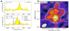 |
Fig. 4. Panel a: [CII] spectra (yellow) of the individual galaxy components in the merging system are shown: #A in the upper panel, and the combined spectrum of #B, #C, #D in the lower panel. Solid coloured lines represent Gaussian models of the spectra. Panel b: velocity-integrated [CII] flux map obtained integrating the broad velocity range [ − 500 : +500] km s−1, to visualise the total [CII] emission arising from the full system. Black plus symbols show the rest-frame UV centroids of #A and #B. The dashed blue ellipses defined in Fig. 3 (see Sect. 3.3) are shown for reference. Black solid (dashed) contours indicate the positive (negative) significance levels at [2, 4, 6]σ of [CII] flux, where σ[CII] = 0.13 Jy km s−1 beam−1. Green contours indicate (as in Fig. 3) the FIR-continuum significance levels [3, 4]σ, where σcont = 59 μJy beam−1. The grey solid line indicates the 1σ level of the total [CII] emission, and it is used as a reference aperture for the extraction of the full [CII] spectrum arising from the entire system. The ALMA beam size is given in the bottom-left corner. A scale of 15 kpc is shown on the right side. North is up and east is to the left. |
To visualise the total [CII] emission arising from the full system, we produced a velocity-integrated flux map by collapsing the spectral channels in the velocity range [ − 500 : +500] km s−1, using a consistent zref as discussed above. Such a broad velocity domain is needed to safely include the four detected [CII]-emitting galaxies (see spectra in Fig. 4a). The resulting velocity-integrated [CII] map is shown in Fig. 4b. We find a very large [CII]-emitting structure extending on circumgalactic scales, with a projected diameter of ∼30 kpc. Such a metal-enriched gaseous structure encloses the single-galaxy components, and shows a large amount of [CII] arising from regions significantly displaced (≳10 kpc) from the rest-frame UV/optical counterparts, especially along the direction orthogonal to the #A–#B axis. However, because of its 2D nature, the [CII] flux map shown in Fig. 4b suffers from the dilution of signal emitted by sources with a width much narrower than the velocity-filter adopted for the spectral integration. Therefore, to better visualise the 3D distribution of the gaseous structure, we produced two position-velocity (PV) diagrams, one extracted along the #A–#B axis (Fig. 5a), and the other along the orthogonal direction, centred on #B (Fig. 5b). Both diagrams highlight the complex morpho-kinematic structure of the system, clearly showing the presence of circumgalactic tails around the interacting galaxies (see e.g. the [CII]-emitting regions labelled “CGM” in both panels of Fig. 5).
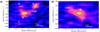 |
Fig. 5. Panel a: PV diagrams taken along the common axis between the [CII]-flux centroids of #A–#B, and the orthogonal axis (panel b), with an averaging width of five pixels. Black contours indicate the [3, 6] σ significance levels, where σpv ∼ 0.3 mJy beam−1 in both cases. A scale of 7 kpc is shown in the lower right. |
One important piece of information is the net contribution of the four interacting galaxies themselves to the overall [CII] emission arising from the extended gaseous structure. To distinguish between the relative “galaxy” and “CGM” [CII] budgets, we extracted a spectrum of the total [CII]-emitting system from a region within the 1-σ contour of the velocity-integrated map (see grey solid line in Fig. 4b), and compare it with the sum of the single #A, #B, #C, and #D spectra (see Fig. 6a). We note that, due to the dynamical complexity of our object, such a procedure is more accurate than extracting relative budgets directly from the velocity-integrated map, because of the limitations of the latter, as discussed above. We find that the full [CII]-emitting structure has a total luminosity of ![$ L_{\mathrm{[CII]}}^{\mathrm{tot}} = 2.3(\pm 0.2) \times 10^9 \, {L_\odot} $](/articles/aa/full_html/2020/11/aa38284-20/aa38284-20-eq20.gif) , meaning ∼2 times larger than the sum of the [CII]-emitting galaxies. This implies that about 50(±6)% (see Fig. 6b) of the total [CII] luminosity resides between the individual components,
, meaning ∼2 times larger than the sum of the [CII]-emitting galaxies. This implies that about 50(±6)% (see Fig. 6b) of the total [CII] luminosity resides between the individual components, ![$ L_{\mathrm{[CII]}}^{\mathrm{CGM}} = 1.1 (\pm 0.2) \times 10^9\, {L_\odot} $](/articles/aa/full_html/2020/11/aa38284-20/aa38284-20-eq21.gif) , in a sort of circumgalactic and metal-rich gaseous envelope around the merging galaxies. This fraction of [CII] emission arising from the CGM is larger than what is typically found around the few individual normal isolated galaxies (i.e. with no evident signs of major/minor mergers) that show a [CII] halo (see Fujimoto et al. 2020), suggesting a link with the merging nature of our system.
, in a sort of circumgalactic and metal-rich gaseous envelope around the merging galaxies. This fraction of [CII] emission arising from the CGM is larger than what is typically found around the few individual normal isolated galaxies (i.e. with no evident signs of major/minor mergers) that show a [CII] halo (see Fujimoto et al. 2020), suggesting a link with the merging nature of our system.
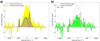 |
Fig. 6. Spectrum of the total [CII] emission arising from the full system (Sect. 3.3), yellow in panel a and red in panel b, is compared with the sum (black shaded area) of the Gaussian models of individual galaxy components (coloured solid lines in panel a) and with their difference (green spectrum in panel b), corresponding to the emission arising from the circumgalactic gaseous envelope. |
In the next section, we discuss possible mechanisms responsible for such large amounts of circumgalactic [CII] emission.
4. Discussion: gas mixing in the CGM
4.1. Dynamical interactions and shocks
A natural scenario to explain the origin of the luminous gaseous envelope is that the circumgalactic [CII] traces the gas stripped during gravitational encounters occurring in the dense merging system. Strong dynamical interactions between the four galaxies might therefore remove a significant amount of interstellar gas from their outer regions, polluting the CGM with chemically enriched material, and producing the complex morphology (see Figs. 3 and 4a) and kinematics (see Fig. 5) observed.
In this scenario, our observations could be a high-z analogue of local studies of circumgalactic stripped [CII] in local groups. For instance, Appleton et al. (2013) detected a broad [CII] emission arising from an extended shocked filament (∼35 kpc) produced by supersonic collisions between galaxies in the compact local group, Stephan’s Quintet. They observed very large [CII]/polycyclic aromatic hydrocarbon (PAH) and [CII]/FIR ratios, which cannot be accounted for by [CII] emission originating from photo-dissociation regions (PDRs: Stacey et al. 1991, 2010) only, and suggest that circumgalactic [CII] can be excited by the dissipation of mechanical energy (turbulence and shocks) injected by strong dynamical interactions. Such a mechanism is expected to be more frequent and more disruptive at high-z because of (i) higher merger rates (e.g. Conselice 2006; Wetzel et al. 2009; Lotz et al. 2011) and (ii) generally higher gas fractions (e.g. Santini et al. 2014; Dessauges-Zavadsky et al. 2017; Schinnerer et al. 2016; Scoville et al. 2017; Tacconi et al. 2018), and might also explain previous similar observations of extended [CII] emission around multi-component systems at z ∼ 5 (see HZ6 and HZ8 in Capak et al. 2015; Faisst et al. 2017). We will further explore this hypothesis by extending similar morpho-spectral decomposition analyses presented in this paper to other major/minor merging systems in the ALPINE survey (see a discussion on ALPINE mergers in Le Fèvre et al. 2020 and Jones et al. 2020) in future works.
Interestingly, since (as discussed in Sect. 3.2) our merging system is close to an overdensity peak of the proto-cluster PClJ1001 + 0220 at z ∼ 4.57 (see Lemaux et al. 2018), the merger-induced CGM pollution might be a natural channel to feed and enrich the nascent proto-intracluster medium (ICM: see e.g. Cucciati et al. 2014, Tozzi et al. 2003, and a recent review by Overzier 2016). Thus, our results could be some of the first observational evidence at high redshift that mergers and gas stripping are key mechanisms in driving the build-up and the chemical evolution of the ICM, as predicted by models and numerical simulations (see e.g. Gnedin 1998; Toniazzo & Schindler 2001; Tornatore et al. 2004; De Lucia et al. 2004; Kapferer et al. 2007). Also, the peculiar location of our system within a large-scale overdense structure suggests that it sits in proximity to a cosmic web node where several filaments from the IGM might be feeding into it. Shocks are predicted to occur as the intergalactic gas accretes onto massive galaxies and mixes with their CGM (see e.g. Birnboim & Dekel 2003; Kereš et al. 2009), and they likely contribute to the [CII] excitation. To quantitatively assess this scenario, we will need new deep observations of the large-scale environment tracing the hydrogen gas, representing the bulk of the intergalactic streams, that can be traced, for example, through Lyα with MUSE (which has a field of view of ∼400 kpc at this redshift).
4.2. Galactic outflows
Another possible contributing scenario is that a fraction of the circumgalactic metal-enriched gas traced by the extended [CII] envelope is expelled from the internal ISM of galaxies through galactic outflows. Evidence of star formation-driven winds has recently been observed at z > 4 (see Sugahara et al. 2019; Faisst et al. 2020; Ginolfi et al. 2020; Cassata et al. 2020), and repeated episodes of outflows are thought to be responsible for the origin of diffuse [CII] halos (∼20 kpc) detected around isolated massive star-forming high-z galaxies (see Faisst et al. 2017; Fujimoto et al. 2019, 2020; Ginolfi et al. 2020; Pizzati et al. 2020). However, a rough estimate suggests that outflows might not be the dominant mechanism for injecting the large amount of circumgalactic cold gas observed in our system (see Figs. 4b and 6). Using the L[CII] − Mgas relation calibrated by Zanella et al. (2018) and the [CII] luminosity arising from the CGM (i.e. about 50% of the total L[CII] (see last paragraph of Sect. 3.3) we obtain a rough estimate of the dense mass of in the [CII] gaseous envelope,  . Then, using typical mass outflow rates of Ṁout ∼ 30 M⊙ yr−1 (as measured by Ginolfi et al. 2020 in the sub-sample of highly star-forming ALPINE galaxies), and assuming that both #A and #B significantly contribute to gas expulsion8, we find that outflows would require at least ∼0.6 Gyr to expel the estimated amount of dense gas in the CGM. We note that this estimate is very conservative, since it is derived under the unlikely assumptions that (i) re-accretion does not occur, and (ii) both #A and #B have constantly had, during their past growth, a sufficient SFR to produce powerful outflows.
4.3. Small faint satellites
A third complementary process would be that part of the extended [CII] emission is induced by the star formation of several small satellites, which are unresolved by our ALMA observations and faint in the rest-frame UV HST images (the few light spots around #A and #B in the HST maps, see Figs. 1a and b, may belong to this category). To estimate the efficiency of this mechanism, we estimated the possible diffuse SFR produced by faint satellites by integrating the rest-frame UV light within an aperture defined as the 1σ level of the [CII] full structure (see grey line in Figs. 1a and 4b), and then subtracting the UV flux arising from regions defined as the blue ellipses (see Sect. 3.3 and Fig. 4b) associated with the individual galaxy components #A, #B, #C, and #D. Using a standard Kennicutt & Evans (2012) calibration, we estimated a total diffuse UV-based  , which is about one order of magnitude lower than expected assuming a L[CII] − SFR relation9 (see e.g. De Looze et al. 2014; Lagache et al. 2018; Schaerer et al. 2020: see a similar calculation in Fujimoto et al. 2019),
 ![$ \mathrm{SFR}_{\mathrm{CGM}}^{\mathrm{[CII]}} \sim 125\,{M_\odot\,\mathrm{yr}^{-1}} $](/articles/aa/full_html/2020/11/aa38284-20/aa38284-20-eq24.gif) . This suggests that, unless the diffuse SFR was exceptionally dust obscured, which is disfavoured by the non-detection of ALMA FIR-continuum (see also Fudamoto et al. 2020, showing that low-mass objects are not expected to have high LIR/LUV), small faint satellites do not significantly account for the detected large circumgalactic [CII] emission.
. This suggests that, unless the diffuse SFR was exceptionally dust obscured, which is disfavoured by the non-detection of ALMA FIR-continuum (see also Fudamoto et al. 2020, showing that low-mass objects are not expected to have high LIR/LUV), small faint satellites do not significantly account for the detected large circumgalactic [CII] emission.
Thus, gas stripping by dynamical interactions (with a possibly relative lower efficiency), galactic outflows, and small faint satellites jointly contribute to the gas mixing and the metal enrichment of the CGM around high-z merging systems. To resolve these mechanisms and quantitatively assess their relative efficiencies, we urge (i) deeper/higher-resolution ALMA FIR-lines mapping and (ii) future rest-frame optical emission line observations with JWST, to be interpreted with tailored zoom-in cosmological simulations (e.g. Kohandel et al. 2019; Pallottini et al. 2019; Graziani et al. 2020).
5. Conclusions
In this work, we present ALMA observations of [CII] and FIR-continuum emission in/around a merging system at z ∼ 4.57, observed as a part of the ALPINE survey (see Le Fèvre et al. 2020; Faisst et al. 2020; Béthermin et al. 2020). Combining information from a rich set of panchromatic ancillary data (including imaging and spectroscopy from rest-frame UV to the near-IR; Faisst et al. 2020) with a morpho-spectral decomposition of the ALMA data (see Sect. 3.3), we find the results summarised below.
-
VC_9780 (dubbed #A) and C15_705574 (dubbed #B), with star formation rates
 and
and  , respectively, and similar stellar masses of M⋆ ∼ 1010 M⊙, are undergoing a major merger (stellar mass ratio rmass ∼ 0.9; see Sect. 3.1), at a close projected separation of ∼13 kpc (see Fig. 1), with a small velocity offset of Δv ∼ 270 km s−1. ALMA data reveal the presence of two faint and narrow (FWHM ∼ 50 km s−1) [CII]-emitting satellites (see Fig. 4) close to #B, and most likely in the process of orbiting around (or accreting into) it. We find that our merging system belongs to the proto-cluster PClJ1001 + 0220 (Lemaux et al. 2018: see Sect. 3.2), and it is coincident to one of its overdensity peaks (see Fig. 2).
 -
We produced a velocity-integrated map collapsing the broad velocity range [−500 : +500] km s−1 to visualise the total [CII] emission arising from the full system, and find a very large structure extending over circumgalactic scales, out to a diameter scale of ∼30 kpc (see Fig. 4), surrounding the galaxy components. A fraction of [CII] flux appears significantly displaced (≳10 kpc) from the rest-frame UV counterparts of #A and #B. Both flux maps (see Figs. 3 and 4) and PV diagrams (see Fig. 5) indicate a disturbed morphology and complex kinematics of the overall gas structure.
-
We compare the flux arising from the extended [CII]-emitting region with the sum of [CII] fluxes emitted by single galaxies, and find that about 50% of the total emission arises from a gaseous envelope distributed between the individual components of the system (see Fig. 6 and discussion about possibly similar objects in Faisst et al. 2017). While a contribution of processed material expelled by galactic outflows (see e.g., Ginolfi et al. 2020; Fujimoto et al. 2020) and SFR-induced [CII] emitted by small faint satellites should be not negligible, we argue that most of the detected circumgalactic emission originates from the effect of gas stripping induced by strong gravitational interactions (see discussion in Sect. 4), in analogy with observations of tidal tails of shock-excited [CII] in local compact groups (e.g. Appleton et al. 2013). This might also represent a natural channel to feed and enrich the ICM in the large-scale proto-cluster environment surrounding our system (see Sect. 3.2 and Fig. 2).
All together, our findings suggest that dynamical interactions at high-z can be an efficient mechanism for extracting gas out of galaxies and mixing the CGM with chemically evolved material. Deeper and higher resolution ALMA data, as well as future JWST rest-frame optical emission line observations, will be necessary to study, in more detail, the key role of mergers in the baryon cycle of distant galaxies.
ID = 705574 in the COSMOS2015 catalogue (Laigle et al. 2016).
We note that the actual velocity offsets are likely to be even lower, since the redshift measured through Lyα can be off by few hundreds of km s−1 towards the red (see e.g. Shapley et al. 2003; Trainor et al. 2015; Verhamme et al. 2018; Cassata et al. 2020).
We assume that the contribution from the satellite galaxies #C and #D to gas-pollution through outflows is negligible. Indeed, from their L[CII], using the L[CII] − SFR relation calibrated by Schaerer et al. 2020, we find SFRs ≲ 10 M⊙ yr−1, and galaxies with such a low SFR at high-z have been reported to not show signatures of prominent outflows (e.g. Ginolfi et al. 2020), nor signs of significant amounts of circumgalactic emission (e.g. Ginolfi et al. 2020; Fujimoto et al. 2020).
We used three different calibrations, which give consistent results: (i) ![$ \mathrm{SFR}_{\mathrm{CGM}}^{\mathrm{[CII]}} \sim 129 \pm 46\,{M_\odot\,\mathrm{yr}^{-1}} $](/articles/aa/full_html/2020/11/aa38284-20/aa38284-20-eq27.gif) from Schaerer et al. (2020), calibrated for galaxies at 4 < z < 6; (ii)
from Schaerer et al. (2020), calibrated for galaxies at 4 < z < 6; (ii) ![$ \mathrm{SFR}_{\mathrm{CGM}}^{\mathrm{[CII]}} \sim 124 \pm 40\,{M_\odot\,\mathrm{yr}^{-1}} $](/articles/aa/full_html/2020/11/aa38284-20/aa38284-20-eq28.gif) from De Looze et al. (2014), calibrated for local galaxies; (iii)
from De Looze et al. (2014), calibrated for local galaxies; (iii) ![$ \mathrm{SFR}_{\mathrm{CGM}}^{\mathrm{[CII]}} \sim 125\,{M_\odot\,\mathrm{yr}^{-1}} $](/articles/aa/full_html/2020/11/aa38284-20/aa38284-20-eq29.gif) from the model of Lagache et al. (2018). Errors on the SFR were computed using the uncertainties on the parameters of the relations.
from the model of Lagache et al. (2018). Errors on the SFR were computed using the uncertainties on the parameters of the relations.
Acknowledgments
The authors would like to thank the anonymous referee for her/his useful suggestions. This paper is based on data obtained with the ALMA Observatory, under Large Program 2017.1.00428.L. ALMA is a partnership of ESO (representing its member states), NSF (USA) and NINS (Japan), together with NRC (Canada), MOST and ASIAA (Taiwan), and KASI (Republic of Korea), in cooperation with the Republic of Chile. The Joint ALMA Observatory is operated by ESO, AUI/NRAO and NAOJ. G.C.J.and R.M. acknowledge the ERC Advanced Grant 695671 “QUENCH” and support by the Science and Technology Facilities Council (STFC). C.G. and M.T. acknowledge the support from a grant PRIN MIUR 2017. S.C. acknowledges support from the ERC Advanced Grant INTERSTELLAR H2020/740120. The Cosmic Dawn Center is funded by the Danish National Research Foundation under grant No. 140. Some of the material presented in this paper is based upon work supported by the National Science Foundation under Grant No. 1908422. This program receives financial support from the French CNRS-INSU Programme National Cosmologie et Galaxies. This paper is dedicated to the memory of Olivier Le Fèvre, PI of the ALPINE survey.
References
- Anglés-Alcázar, D., Faucher-Giguère, C.-A., Kereš, D., et al. 2017, MNRAS, 470, 4698 [NASA ADS] [CrossRef] [Google Scholar]
- Appleton, P. N., Guillard, P., Boulanger, F., et al. 2013, ApJ, 777, 66 [NASA ADS] [CrossRef] [Google Scholar]
- Arnouts, S., & Ilbert, O. 2011, LePHARE: Photometric Analysis for Redshift Estimate [Google Scholar]
- Arnouts, S., Cristiani, S., Moscardini, L., et al. 1999, MNRAS, 310, 540 [NASA ADS] [CrossRef] [Google Scholar]
- Barnes, J. E., & Hernquist, L. E. 1991, ApJ, 370, L65 [NASA ADS] [CrossRef] [Google Scholar]
- Béthermin, M., Fudamoto, Y., Ginolfi, M. et al. 2020, A&A, 643, A2 [CrossRef] [EDP Sciences] [Google Scholar]
- Birnboim, Y., & Dekel, A. 2003, MNRAS, 345, 349 [NASA ADS] [CrossRef] [Google Scholar]
- Boselli, A., Boissier, S., Cortese, L., et al. 2006, ApJ, 651, 811 [NASA ADS] [CrossRef] [Google Scholar]
- Bournaud, F., Chapon, D., Teyssier, R., et al. 2011, ApJ, 730, 4 [NASA ADS] [CrossRef] [Google Scholar]
- Bower, R. G., Benson, A. J., Malbon, R., et al. 2006, MNRAS, 370, 645 [NASA ADS] [CrossRef] [Google Scholar]
- Bradač, M., Garcia-Appadoo, D., Huang, K.-H., et al. 2017, ApJ, 836, L2 [NASA ADS] [CrossRef] [Google Scholar]
- Bridge, C. R., Carlberg, R. G., & Sullivan, M. 2010, ApJ, 709, 1067 [NASA ADS] [CrossRef] [Google Scholar]
- Calzetti, D., Armus, L., Bohlin, R. C., et al. 2000, ApJ, 533, 682 [NASA ADS] [CrossRef] [Google Scholar]
- Capak, P. L., Carilli, C., Jones, G., et al. 2015, Nature, 522, 455 [NASA ADS] [CrossRef] [Google Scholar]
- Carilli, C. L., & Walter, F. 2013, ARA&A, 51, 105 [NASA ADS] [CrossRef] [EDP Sciences] [Google Scholar]
- Carniani, S., Maiolino, R., Smit, R., & Amorín, R. 2018a, ApJ, 854, L7 [NASA ADS] [CrossRef] [Google Scholar]
- Carniani, S., Maiolino, R., Amorin, R., et al. 2018b, MNRAS, 478, 1170 [NASA ADS] [CrossRef] [Google Scholar]
- Carniani, S., Ferrara, A., Maiolino, R., et al. 2020, MNRAS, submitted [arXiv:2006.09402] [Google Scholar]
- Cassata, P., Morselli, L., Faisst, A., et al. 2020, A&A, 643, A6 [CrossRef] [EDP Sciences] [Google Scholar]
- Chabrier, G. 2003, PASP, 115, 763 [Google Scholar]
- Conselice, C. J. 2006, ApJ, 638, 686 [NASA ADS] [CrossRef] [Google Scholar]
- Cormier, D., Lebouteiller, V., Madden, S. C., et al. 2012, A&A, 548, A20 [NASA ADS] [CrossRef] [EDP Sciences] [Google Scholar]
- Cucciati, O., Zamorani, G., Lemaux, B. C., et al. 2014, A&A, 570, A16 [NASA ADS] [CrossRef] [EDP Sciences] [Google Scholar]
- Cucciati, O., Lemaux, B. C., Zamorani, G., et al. 2018, A&A, 619, A49 [NASA ADS] [CrossRef] [EDP Sciences] [Google Scholar]
- Daddi, E., Elbaz, D., Walter, F., et al. 2010, ApJ, 714, L118 [Google Scholar]
- Decarli, R., Dotti, M., Bañados, E., et al. 2019, ApJ, 880, 157 [NASA ADS] [CrossRef] [Google Scholar]
- Dekel, A., Birnboim, Y., Engel, G., et al. 2009, Nature, 457, 451 [Google Scholar]
- De Looze, I., Cormier, D., Lebouteiller, V., et al. 2014, A&A, 568, A62 [NASA ADS] [CrossRef] [EDP Sciences] [Google Scholar]
- De Lucia, G., Kauffmann, G., & White, S. D. M. 2004, MNRAS, 349, 1101 [NASA ADS] [CrossRef] [Google Scholar]
- Dessauges-Zavadsky, M., Zamojski, M., Rujopakarn, W., et al. 2017, A&A, 605, A81 [NASA ADS] [CrossRef] [EDP Sciences] [Google Scholar]
- Diener, C., Lilly, S. J., Knobel, C., et al. 2013, ApJ, 765, 109 [NASA ADS] [CrossRef] [Google Scholar]
- Diener, C., Lilly, S. J., Ledoux, C., et al. 2015, ApJ, 802, 31 [NASA ADS] [CrossRef] [Google Scholar]
- Di Matteo, T., Springel, V., & Hernquist, L. 2005, Nature, 433, 604 [NASA ADS] [CrossRef] [PubMed] [Google Scholar]
- Di Matteo, P., Bournaud, F., Martig, M., et al. 2008, A&A, 492, 31 [NASA ADS] [CrossRef] [EDP Sciences] [Google Scholar]
- Elmegreen, B. G. 2000, ApJ, 530, 277 [NASA ADS] [CrossRef] [Google Scholar]
- Faber, S. M., Phillips, A. C., & Kibrick, R. I. 2003, The DEIMOS Spectrograph for the Keck II Telescope: Integration and Testing, eds. M. Iye, & A. F. M. Moorwood, SPIE Conf. Ser., 4841, 1657 [Google Scholar]
- Faisst, A. L., Capak, P. L., Yan, L., et al. 2017, ApJ, 847, 21 [NASA ADS] [CrossRef] [Google Scholar]
- Faisst, A. L., Schaerer, D., Lemaux, B. C., et al. 2020, ApJS, 247, 61 [Google Scholar]
- Ferrara, A., Vallini, L., Pallottini, A., et al. 2019, MNRAS, 489, 1 [NASA ADS] [CrossRef] [Google Scholar]
- Fossati, M., Fumagalli, M., Gavazzi, G., et al. 2019, MNRAS, 484, 2212 [NASA ADS] [CrossRef] [Google Scholar]
- Fudamoto, Y., Oesch, P. A., Faisst, A., et al. 2020, A&A, 643, A4 [CrossRef] [EDP Sciences] [Google Scholar]
- Fujimoto, S., Ouchi, M., Ferrara, A., et al. 2019, ApJ, 887, 107 [NASA ADS] [CrossRef] [Google Scholar]
- Fujimoto, S., Silverman, J. D., Béthermin, M., et al. 2020, ApJ, 900, 1 [CrossRef] [Google Scholar]
- García-Burillo, S., Combes, F., Schinnerer, E., Boone, F., & Hunt, L. K. 2005, A&A, 441, 1011 [NASA ADS] [CrossRef] [EDP Sciences] [Google Scholar]
- Ginolfi, M., Schneider, R., Valiante, R., et al. 2019, MNRAS, 483, 1256 [CrossRef] [Google Scholar]
- Ginolfi, M., Jones, G. C., Béthermin, M., et al. 2020, A&A, 633, A90 [CrossRef] [EDP Sciences] [Google Scholar]
- Gnedin, N. Y. 1998, MNRAS, 294, 407 [NASA ADS] [CrossRef] [Google Scholar]
- Graziani, L., Schneider, R., Ginolfi, M., et al. 2020, MNRAS, 494, 1071 [CrossRef] [Google Scholar]
- Gunn, J. E., Gott, J., & Richard, I. 1972, ApJ, 176, 1 [NASA ADS] [CrossRef] [Google Scholar]
- Guo, R., Hao, C.-N., Xia, X. Y., Mao, S., & Shi, Y. 2016, ApJ, 826, 30 [NASA ADS] [CrossRef] [Google Scholar]
- Hani, M. H., Sparre, M., Ellison, S. L., Torrey, P., & Vogelsberger, M. 2018, MNRAS, 475, 1160 [CrossRef] [Google Scholar]
- Hopkins, P. F., Hernquist, L., Cox, T. J., et al. 2006, ApJS, 163, 1 [Google Scholar]
- Hopkins, P. F., Bundy, K., Croton, D., et al. 2010, ApJ, 715, 202 [NASA ADS] [CrossRef] [Google Scholar]
- Hung, D., Lemaux, B. C., Gal, R. R., et al. 2020, MNRAS, 491, 5524 [CrossRef] [Google Scholar]
- Ilbert, O., Arnouts, S., McCracken, H. J., et al. 2006, A&A, 457, 841 [NASA ADS] [CrossRef] [EDP Sciences] [Google Scholar]
- Inoue, K. T., Minezaki, T., Matsushita, S., & Chiba, M. 2016, MNRAS, 457, 2936 [CrossRef] [Google Scholar]
- Jones, G. C., Carilli, C. L., Shao, Y., et al. 2017, ApJ, 850, 180 [NASA ADS] [CrossRef] [Google Scholar]
- Jones, G. C., Béthermin, M., Fudamoto, Y., et al. 2020, MNRAS, 491, L18 [Google Scholar]
- Kapferer, W., Kronberger, T., Weratschnig, J., et al. 2007, A&A, 466, 813 [NASA ADS] [CrossRef] [EDP Sciences] [Google Scholar]
- Kennicutt, R. C., & Evans, N. J. 2012, ARA&A, 50, 531 [NASA ADS] [CrossRef] [Google Scholar]
- Kereš, D., Katz, N., Fardal, M., Davé, R., & Weinberg, D. H. 2009, MNRAS, 395, 160 [NASA ADS] [CrossRef] [Google Scholar]
- Koekemoer, A. M., Aussel, H., Calzetti, D., et al. 2007, ApJS, 172, 196 [NASA ADS] [CrossRef] [Google Scholar]
- Kohandel, M., Pallottini, A., Ferrara, A., et al. 2019, MNRAS, 487, 3007 [NASA ADS] [CrossRef] [Google Scholar]
- Lagache, G., Cousin, M., & Chatzikos, M. 2018, A&A, 609, A130 [NASA ADS] [CrossRef] [EDP Sciences] [Google Scholar]
- Laigle, C., McCracken, H. J., Ilbert, O., et al. 2016, ApJS, 224, 24 [NASA ADS] [CrossRef] [Google Scholar]
- Le Fèvre, O., Tasca, L. A. M., Cassata, P., et al. 2015, A&A, 576, A79 [NASA ADS] [CrossRef] [EDP Sciences] [Google Scholar]
- Le Fèvre, O., Béthermin, M., Faisst, A., et al. 2020, A&A, 643, A1 [CrossRef] [EDP Sciences] [Google Scholar]
- Lemaux, B. C., Tomczak, A. R., Lubin, L. M., et al. 2017, MNRAS, 472, 419 [NASA ADS] [CrossRef] [Google Scholar]
- Lemaux, B. C., Le Fèvre, O., Cucciati, O., et al. 2018, A&A, 615, A77 [NASA ADS] [CrossRef] [EDP Sciences] [Google Scholar]
- Lemaux, B. C., Tomczak, A. R., Lubin, L. M., et al. 2019, MNRAS, 490, 1231 [NASA ADS] [CrossRef] [Google Scholar]
- Lilly, S. J., Le Fèvre, O., Renzini, A., et al. 2007, ApJS, 172, 70 [NASA ADS] [CrossRef] [Google Scholar]
- Lilly, S. J., Le Brun, V., Maier, C., et al. 2009, ApJS, 184, 218 [Google Scholar]
- Lilly, S. J., Carollo, C. M., Pipino, A., Renzini, A., & Peng, Y. 2013, ApJ, 772, 119 [NASA ADS] [CrossRef] [Google Scholar]
- Lotz, J. M., Jonsson, P., Cox, T. J., & Primack, J. R. 2010, MNRAS, 404, 575 [Google Scholar]
- Lotz, J. M., Jonsson, P., Cox, T. J., et al. 2011, ApJ, 742, 103 [NASA ADS] [CrossRef] [Google Scholar]
- Maiolino, R., Carniani, S., Fontana, A., et al. 2015, MNRAS, 452, 54 [NASA ADS] [CrossRef] [Google Scholar]
- Marrone, D. P., Spilker, J. S., Hayward, C. C., et al. 2018, Nature, 553, 51 [NASA ADS] [CrossRef] [Google Scholar]
- Matthee, J., Sobral, D., Boone, F., et al. 2017, ApJ, 851, 145 [NASA ADS] [CrossRef] [Google Scholar]
- Matthee, J., Sobral, D., Boogaard, L. A., et al. 2019, ApJ, 881, 124 [NASA ADS] [CrossRef] [Google Scholar]
- McCracken, H. J., Milvang-Jensen, B., Dunlop, J., et al. 2012, A&A, 544, A156 [NASA ADS] [CrossRef] [EDP Sciences] [Google Scholar]
- McMullin, J. P., Waters, B., Schiebel, D., Young, W., & Golap, K. 2007, CASA Architecture and Applications, eds. R. A. Shaw, F. Hill, & D. J. Bell, ASP Conf. Ser., 376, 127 [Google Scholar]
- Moretti, A., Paladino, R., Poggianti, B. M., et al. 2018, MNRAS, 480, 2508 [Google Scholar]
- Nelson, D., Genel, S., Vogelsberger, M., et al. 2015, MNRAS, 448, 59 [NASA ADS] [CrossRef] [Google Scholar]
- Oteo, I., Ivison, R. J., Dunne, L., et al. 2016, ApJ, 827, 34 [NASA ADS] [CrossRef] [Google Scholar]
- Overzier, R. A. 2016, A&ARv, 24, 14 [NASA ADS] [CrossRef] [Google Scholar]
- Pallottini, A., Ferrara, A., Decataldo, D., et al. 2019, MNRAS, 487, 1689 [NASA ADS] [CrossRef] [Google Scholar]
- Pavesi, R., Riechers, D. A., Sharon, C. E., et al. 2018, ApJ, 861, 43 [NASA ADS] [CrossRef] [Google Scholar]
- Pentericci, L., Carniani, S., Castellano, M., et al. 2016, ApJ, 829, L11 [NASA ADS] [CrossRef] [Google Scholar]
- Pizzati, E., Ferrara, A., Pallottini, A., et al. 2020, MNRAS, 495, 160 [CrossRef] [Google Scholar]
- Poggianti, B. M., Gullieuszik, M., Moretti, A., et al. 2017, The Messenger, 170, 29 [Google Scholar]
- Poggianti, B. M., Ignesti, A., Gitti, M., et al. 2019, ApJ, 887, 155 [NASA ADS] [CrossRef] [Google Scholar]
- Riechers, D. A., Leung, T. K. D., Ivison, R. J., et al. 2017, ApJ, 850, 1 [Google Scholar]
- Rodighiero, G., Daddi, E., Baronchelli, I., et al. 2011, ApJ, 739, L40 [NASA ADS] [CrossRef] [Google Scholar]
- Sanders, D. B., & Mirabel, I. F. 1996, ARA&A, 34, 749 [NASA ADS] [CrossRef] [Google Scholar]
- Santini, P., Maiolino, R., Magnelli, B., et al. 2014, A&A, 562, A30 [NASA ADS] [CrossRef] [EDP Sciences] [Google Scholar]
- Schaerer, D., Ginolfi, M., Béthermin, M., et al. 2020, A&A, 643, A3 [CrossRef] [EDP Sciences] [Google Scholar]
- Schaye, J., Crain, R. A., Bower, R. G., et al. 2015, MNRAS, 446, 521 [Google Scholar]
- Schinnerer, E., Groves, B., Sargent, M. T., et al. 2016, ApJ, 833, 112 [NASA ADS] [CrossRef] [Google Scholar]
- Scoville, N., Aussel, H., Brusa, M., et al. 2007, ApJS, 172, 1 [NASA ADS] [CrossRef] [Google Scholar]
- Scoville, N., Sheth, K., Aussel, H., et al. 2016, ApJ, 820, 83 [NASA ADS] [CrossRef] [Google Scholar]
- Scoville, N., Lee, N., Vanden Bout, P., et al. 2017, ApJ, 837, 150 [NASA ADS] [CrossRef] [Google Scholar]
- Sérsic, J. L. 1963, Boletin de la Asociacion Argentina de Astronomia La Plata Argentina, 6, 41 [Google Scholar]
- Shapley, A. E., Steidel, C. C., Pettini, M., & Adelberger, K. L. 2003, ApJ, 588, 65 [NASA ADS] [CrossRef] [Google Scholar]
- Speagle, J. S., Steinhardt, C. L., Capak, P. L., & Silverman, J. D. 2014, ApJS, 214, 15 [NASA ADS] [CrossRef] [Google Scholar]
- Stacey, G. J., Geis, N., Genzel, R., et al. 1991, ApJ, 373, 423 [NASA ADS] [CrossRef] [Google Scholar]
- Stacey, G. J., Hailey-Dunsheath, S., Ferkinhoff, C., et al. 2010, ApJ, 724, 957 [NASA ADS] [CrossRef] [Google Scholar]
- Stewart, K. R., Bullock, J. S., Barton, E. J., & Wechsler, R. H. 2009, ApJ, 702, 1005 [NASA ADS] [CrossRef] [Google Scholar]
- Stewart, K. R., Kaufmann, T., Bullock, J. S., et al. 2011, ApJ, 738, 39 [NASA ADS] [CrossRef] [Google Scholar]
- Sugahara, Y., Ouchi, M., Harikane, Y., et al. 2019, ApJ, 886, 29 [NASA ADS] [CrossRef] [Google Scholar]
- Tacconi, L. J., Genzel, R., Saintonge, A., et al. 2018, ApJ, 853, 179 [NASA ADS] [CrossRef] [Google Scholar]
- Tasca, L. A. M., Le Fèvre, O., Ribeiro, B., et al. 2017, A&A, 600, A110 [NASA ADS] [CrossRef] [EDP Sciences] [Google Scholar]
- Tomczak, A. R., Lemaux, B. C., Lubin, L. M., et al. 2017, MNRAS, 472, 3512 [NASA ADS] [CrossRef] [Google Scholar]
- Toniazzo, T., & Schindler, S. 2001, MNRAS, 325, 509 [NASA ADS] [CrossRef] [Google Scholar]
- Tornatore, L., Borgani, S., Matteucci, F., Recchi, S., & Tozzi, P. 2004, MNRAS, 349, L19 [NASA ADS] [CrossRef] [Google Scholar]
- Tozzi, P., Rosati, P., Ettori, S., et al. 2003, ApJ, 593, 705 [NASA ADS] [CrossRef] [Google Scholar]
- Trainor, R. F., Steidel, C. C., Strom, A. L., & Rudie, G. C. 2015, ApJ, 809, 89 [NASA ADS] [CrossRef] [Google Scholar]
- Vallini, L., Gallerani, S., Ferrara, A., & Baek, S. 2013, MNRAS, 433, 1567 [NASA ADS] [CrossRef] [Google Scholar]
- Vallini, L., Ferrara, A., Pallottini, A., & Gallerani, S. 2017, MNRAS, 467, 1300 [NASA ADS] [Google Scholar]
- Velusamy, T., & Langer, W. D. 2014, A&A, 572, A45 [NASA ADS] [CrossRef] [EDP Sciences] [Google Scholar]
- Verhamme, A., Garel, T., Ventou, E., et al. 2018, MNRAS, 478, L60 [Google Scholar]
- Vogelsberger, M., Genel, S., Springel, V., et al. 2014, MNRAS, 444, 1518 [NASA ADS] [CrossRef] [Google Scholar]
- Vulcani, B., Moretti, A., Poggianti, B. M., et al. 2017, ApJ, 850, 163 [CrossRef] [Google Scholar]
- Wen, Z. Z., & Zheng, X. Z. 2016, ApJ, 832, 90 [NASA ADS] [CrossRef] [Google Scholar]
- Wetzel, A. R., Cohn, J. D., & White, M. 2009, MNRAS, 395, 1376 [NASA ADS] [CrossRef] [Google Scholar]
- Zanella, A., Daddi, E., Magdis, G., et al. 2018, MNRAS, 481, 1976 [Google Scholar]
Appendix A: Description of the VMC mapping technique
Here, we briefly describe the VMC mapping technique used to produce Fig. 2, discussed in Sect. 3.2. We refer to Lemaux et al. (2018, and reference therein) for more details.
To reconstruct the density field in a given redshift range, a large number of Monte Carlo iterations of the input spectroscopic and photometric catalogs are run. For each Monte Carlo realisation, we begin with all objects that have spectroscopic information, sampling a random uniform distribution for each object. For a given object, if the sample exceeds the value of a predetermined reliability flag for that redshift, we throw away the spectral redshift and, for that Monte Carlo realisation, rely on the photometric redshift information. If the uniform sampling does not exceed the reliability threshold, we retain the spectral information for that object in that realisation. Then, those objects where the spectral information was disavowed, along with those objects that had no spectral information, have their photometric redshifts tweaked by sampling a reconstruction of their full P(z). Thus, at the end of a given iteration, all objects in the combined spectral and photometric catalog have a set redshift. We then set a redshift boundary to generate the 2D map and Voronoi tessellate over all objects whose redshifts, spectral or photometric, fall within the redshift boundaries. The local density value, ΣVMC, of a given object for a given iteration is the inverse of the area of the Voronoi cell surrounding it. This process is repeated for the set number of Monte Carlo realisations, with the density values of each realisation sampled by a standardised grid of 75 × 75  proper kpc, and the pixel values from all realisations are then median combined. As in other works, we rely here on local overdensity rather than local density as the former has been found to be less sensitive to observational effects. The local overdensity value for each grid point is then computed as
  , where
  is the median ΣVMC for all grid points over which the map was defined, thus excluding an ∼1 arcmin wide border region to mitigate edge effects.
Appendix B: [CII] flux maps of #C and #D
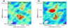 |
Fig. B.1. Panel a: velocity-integrated [CII] maps of #C and panel b: #D, obtained by collapsing the spectral channels corresponding to a 2 × FWHM interval centred on their z[CII] (see spectra in Fig. 4a, and values in Table 1). The velocity ranges used to collapse the datacubes are shown in the top-left corners. The rest-frame UV centroid of #B is indicated with a plus symbol. The dashed blue ellipse defined in Fig. 3 (see Sect. 3.3) is shown for reference. The grey solid line and the black contours indicate the significance level of the [CII] flux emitted by the full system as defined in Fig. 4b. The green solid (dashed) contours indicate the positive (negative) significance levels at [3, 4]σ of the [CII] flux maps of #C panel a and #D panel b. To help the visualisation of panel b, we used a maximum value of surface brightness in the colour-map range as defined by excluding the northern bright spot (corresponding to a fraction of the emission of #A). The ALMA beam size is given in the bottom-left corner. North is up and east is to the left. |
All Tables
All Figures
|
Fig. 1. Panel a: HST/ACS F814W (i-band; Koekemoer et al. 2007), panel b: HST/WFC3 F160W (Faisst et al., in prep.), and panel c: UltraVISTA DR4 Ks-band (McCracken et al. 2012) images of the system. The rest-frame UV positions of VC_9780 (dubbed #A) and C15_705574 (dubbed #B) are highlighted with a yellow square in panel a. The grey contour indicates the extension of the full [CII]-emitting region (see Sect. 3.3). The white bar shows a reference length of 15 kpc. North is up and east is to the left. |
| In the text | |
|
Fig. 2. VMC galaxy overdensity map of the N-E region of the PClJ1001 + 0220 proto-cluster (see details in Sect. 3.2). The VUDS spectral members of the system are indicated with white diamond symbols, while the location of our merging system and a possibly associated additional member observed with DEIMOS are indicated with a cyan star and a blue square, respectively. Overplotted on the map are overdensity isopleths at significance levels of [4, 6, 8, 10, 11.5, 13]σ, where σ is calculated as the RMS fluctuation of the overdensity field over the entire map (see Cucciati et al. 2018; Hung et al. 2020). The map shows that the merging system studied in this work is clearly located close to an overdensity peak of the proto-cluster. The black solid bar shows a reference length of 500 |
| In the text | |
|
Fig. 3. Panel a: velocity-integrated [CII] map of VC_9780 (#A) and panel b: C15_705574 (#B), obtained by collapsing channels (velocity ranges in the upper-left corners) of line-emission in 1″-aperture spectra (see Sect. 3.3) centred on the rest-frame UV centroids of #A and #B (indicated with a black plus symbol). Black solid (dashed) contours indicate the positive (negative) significance levels at [2, 4, 8]σ of [CII] flux, where σ[CII] = 50 mJy km s−1 beam−1 in panel a and σ[CII] = 57 mJy km s−1 beam−1 in panel b. The white contours indicate the positive significance levels at [3, 4]σ of FIR-continuum emission, where σcont = 59 μJy beam−1. No negative contours at the same significance levels were found. The dashed blue ellipses indicate the beam-convolved FWHMx × FWHMy regions obtained by 2D Gaussian models, and correspond to the apertures used to extract the final [CII] spectra of #A and #B (see Sect. 3.3), shown in Fig. 4. The ALMA beam sizes are given in the bottom-left corners. North is up and east is to the left. |
| In the text | |
|
Fig. 4. Panel a: [CII] spectra (yellow) of the individual galaxy components in the merging system are shown: #A in the upper panel, and the combined spectrum of #B, #C, #D in the lower panel. Solid coloured lines represent Gaussian models of the spectra. Panel b: velocity-integrated [CII] flux map obtained integrating the broad velocity range [ − 500 : +500] km s−1, to visualise the total [CII] emission arising from the full system. Black plus symbols show the rest-frame UV centroids of #A and #B. The dashed blue ellipses defined in Fig. 3 (see Sect. 3.3) are shown for reference. Black solid (dashed) contours indicate the positive (negative) significance levels at [2, 4, 6]σ of [CII] flux, where σ[CII] = 0.13 Jy km s−1 beam−1. Green contours indicate (as in Fig. 3) the FIR-continuum significance levels [3, 4]σ, where σcont = 59 μJy beam−1. The grey solid line indicates the 1σ level of the total [CII] emission, and it is used as a reference aperture for the extraction of the full [CII] spectrum arising from the entire system. The ALMA beam size is given in the bottom-left corner. A scale of 15 kpc is shown on the right side. North is up and east is to the left. |
| In the text | |
|
Fig. 5. Panel a: PV diagrams taken along the common axis between the [CII]-flux centroids of #A–#B, and the orthogonal axis (panel b), with an averaging width of five pixels. Black contours indicate the [3, 6] σ significance levels, where σpv ∼ 0.3 mJy beam−1 in both cases. A scale of 7 kpc is shown in the lower right. |
| In the text | |
|
Fig. 6. Spectrum of the total [CII] emission arising from the full system (Sect. 3.3), yellow in panel a and red in panel b, is compared with the sum (black shaded area) of the Gaussian models of individual galaxy components (coloured solid lines in panel a) and with their difference (green spectrum in panel b), corresponding to the emission arising from the circumgalactic gaseous envelope. |
| In the text | |
|
Fig. B.1. Panel a: velocity-integrated [CII] maps of #C and panel b: #D, obtained by collapsing the spectral channels corresponding to a 2 × FWHM interval centred on their z[CII] (see spectra in Fig. 4a, and values in Table 1). The velocity ranges used to collapse the datacubes are shown in the top-left corners. The rest-frame UV centroid of #B is indicated with a plus symbol. The dashed blue ellipse defined in Fig. 3 (see Sect. 3.3) is shown for reference. The grey solid line and the black contours indicate the significance level of the [CII] flux emitted by the full system as defined in Fig. 4b. The green solid (dashed) contours indicate the positive (negative) significance levels at [3, 4]σ of the [CII] flux maps of #C panel a and #D panel b. To help the visualisation of panel b, we used a maximum value of surface brightness in the colour-map range as defined by excluding the northern bright spot (corresponding to a fraction of the emission of #A). The ALMA beam size is given in the bottom-left corner. North is up and east is to the left. |
| In the text | |
Current usage metrics show cumulative count of Article Views (full-text article views including HTML views, PDF and ePub downloads, according to the available data) and Abstracts Views on Vision4Press platform.
Data correspond to usage on the plateform after 2015. The current usage metrics is available 48-96 hours after online publication and is updated daily on week days.
Initial download of the metrics may take a while.