| Issue |
A&A
Volume 641, September 2020
|
|
|---|---|---|
| Article Number | A100 | |
| Number of page(s) | 16 | |
| Section | Planets and planetary systems | |
| DOI | https://doi.org/10.1051/0004-6361/202037454 | |
| Published online | 16 September 2020 | |
A self-consistent method for the simulation of meteor trails with an application to radio observations
1
Vrije Universiteit Brussel, Research Group Electrochemical and Surface Engineering,
Pleinlaan 2,
1050
Brussel,
Belgium
2
von Karman Institute for Fluid Dynamics, Aeronautics and Aerospace Dept.,
Waterloosesteenweg 72,
1640
St.-Genesius-Rode,
Belgium
e-mail: federico.bariselli@vki.ac.be
3
Politecnico di Milano, Dipartimento di Scienze e Tecnologie Aerospaziali,
Via La Masa 34,
20156
Milano,
Italy
4
Université Catholique de Louvain, Inst. of Mechanics, Materials and Civil Engineering,
Place du Levant 2,
1348
Louvain-la-Neuve,
Belgium
Received:
7
January
2020
Accepted:
2
July
2020
Context. Radio-based techniques allow for a meteor detection of 24 h. Electromagnetic waves are scattered by the electrons produced by the ablated species colliding with the incoming air. As the electrons dissipate in the trail, the received signal decays. The interpretation of these measurements entails complex physical modelling of the flow.
Aims. In this work, we present a procedure to compute extensive meteor trails in the rarefied segment of the trajectory. This procedure is a general and standalone methodology, which provides meteor physical parameters at given trajectory conditions, without the need to rely on phenomenological lumped models.
Methods. We started from fully kinetic simulations of the evaporated gas that describe the nonequilibrium in the flow and the ionisation collisions experienced by metals in their encounter with air molecules. These simulations were employed as initial conditions for performing detailed chemical and multicomponent diffusion calculations of the extended trail, in order to study the processes which lead to the extinction of the plasma. In particular, we focused on the evolution of the trail generated by a 1 mm meteoroid flying at 32 km s−1, above 80 km. We retrieved the ambipolar diffusion coefficient and the electron line density and compared the outcome of our computations with classical results and observational fittings. Finally, the electron field was employed to estimate the resulting reflected signal, using classical radio-echo theory for underdense meteors.
Results. A global and constant diffusion coefficient is sufficient to reproduce numerical profiles. A good agreement is found when we compare the extracted diffusion coefficients with theory and observations.
Key words: meteorites, meteors, meteoroids / methods: numerical / plasmas / scattering
© ESO 2020
1 Introduction
Among the various experimental strategies for the observation of meteors, radar- and radio-based techniques (Kaiser 1953; McKinley 1961) have proved to be a simple yet valuable tool for collecting large amounts of data, 24 h a day regardless of the visibility conditions. The data obtained comprise trajectory information, such as the flight velocity, quantities related to the physical state of the meteor vapour, for example, its degree of ionisation (Hocking et al. 2001; Weryk & Brown 2013), or indirect measurements of the atmospheric conditions, such as pressure and temperature (Hocking et al. 1997; Cervera & Reid 2000).
The Belgian Institute for Space Aeronomy has put in place an experiment, the Belgian RAdio Meteor Stations (BRAMS) network, to predict the velocity, trajectory, and mass of meteors. This network consists of a radio transmitter emitting at 49.97 MHz and a series of receivers spread all over Belgium to collect and standardise meteor observations (Lamy et al. 2011). Employing the forward-scattering technique (Forsyth & Vogan 1955), these radio stations can detect free electron densities in the meteoroid trail, which are initially produced by the hyperthermal collisions of the ablated species with the incoming freestream air (Dressler & Murad 2001).
When the density of the free electrons is weak, the incident radio wave can propagate in the ionised gas, where it is scattered by the individual electrons. Astronomers refer to this condition as an underdense reflection. Signals from underdense meteors last no more than a few tenths of a second, and they are observed the most. For these events, the theory indicates that the mass of the object is proportional to the amplitude of the echo, and its duration, which is strictly linked to the deionisation process in the plasma trail, is proportional to the electron line density at the reflection point (McKinley 1961). Figure 1 shows the example of a spectrogram recorded by BRAMS, which was obtained performing a discrete Fourier transform of the raw audio signal over a period of 5 min, during which nine underdense meteor echoes were detected.
Therefore, the ability to calculate the ionisation intensity and distribution, as well as the rate of dissipation of the plasma trail, becomes essential for the correct interpretation of the radio signal. Each improvement in the modelling is expected to impact not only the comprehension of the physical problem but also the estimates on mass fluxes and the statistical outcome of the collected meteor data.
As regards the first point, the modelling of the electron density represents a primary source of uncertainty in the interpretation of radar and radio echoes because it relies on lumped models derived under the assumption of free molecular flow and on the definition of an ionisation efficiency (Jones 1997). In a recent paper (Bariselli et al. 2020), the present authors have performed numerical analysis of the flow around a small meteoroid in a wide range of conditions, and they have shown the major drawbacks of such a simplified approach, one for all, the fact that it does not take into account the degree of rarefaction of flow.
On the other hand, the decay of the signal is mostly linked to the evolution of the free electrons in the trail, and classically it has been studied considering constant ambipolar diffusion and a thermalised chemistry mechanism (Baggaley 2002). In their pioneering work, Baggaley & Cummack (1974) solved a system of diffusion equations in cylindrical coordinates. There, the initial condition was assumed to be a Gaussian radial distribution of the meteoritic atomic ions, which were left as the only constituents of the starting mixture.
The same approach, along with a simplified mixture composed of one single synthetic meteoric element, M, and its oxide ions, MO+, MO , was used to study the echo duration produced in overdense meteors (Baggaley 1978). In these studies, the role of ozone as the controlling neutral gas was recognised, and two-body dissociative recombination was identified as the leading reaction for chemical neutralisation. The initial explanation for which electron attachment could play a significant role in this process was dispelled. Moreover, chemistry was found to be a relevant dissipation mechanism only at altitudes below 80 km, where collisions are more frequent, with diffusion becoming dominant high in the atmosphere.
Although a fairly complete chemical mechanism was considered in these works, the diffusion process was modelled by assuming a common and constant ambipolar diffusion coefficient computed for positive ions moving through a N2 –O2 mixture. The treatment on ionic diffusion in meteor trains was discussed in another work by Jones & Jones (1990) for a binary mixture of ions as they suggested that differential diffusion among species may influence ion chemistry in dense plasma trails. However, no numerical solutions based on the presented results were attained. Dimant & Oppenheim (2006) solved the diffusion equation of the thermalised trail by considering the spatial distribution and evolution of the ambipolar electric field. Additionally, they treated the effects of the background plasma, neutral atmosphere, and geomagneticfield. Ion and electron temperatures were considered constant. In this regard, the thermalisation of the trail was studied by Baggaley & Webb (1977), considering a two-temperature model. The authors showed how free electrons seem to achieve thermal equilibrium with the ambient gas at timescales lower than a tenth of a second.
Numerical computations of the trail offer a set of challenges. An important one concerns its vast extent, which can reach kilometres in length, while the transverse dimension stays of the order of metres. The resulting computational grids are likely to be extremely heavy, if not heavily deformed, and computational resources are easily overwhelmed. Therefore, plasma and gas dynamics simulations have been performed following a variety of methodologies, ad-hoc assumptions and different levels of approximation, depending on the focus of the study. The Direct Simulation Monte Carlo (DSMC) method was employed by Boyd (1998) to obtain nonequilibrium simulations of the vapour in a 40 m trail in order to investigate the relaxation of the rotational degrees of freedom. Zinn et al. (2004) developed a coupled radiative-hydrodynamic code for the cylindrical expansion of the gas in the trail of a fireball, tracking the chemical evolution and temperature distributions in the first 200 m. Finally, Oppenheim & Dimant (2015) studied the diffusion of the plasma column and the development of turbulence in the presence of a background wind using a three-dimensional Particle-In-Cell (PIC) code over a 100 m long domain.
In this work, we present a self-consistent procedure in four steps to compute extensive meteor plasma trails resulting from the ablation process of meteoroid material in the rarefied segment of the entry trajectory. This procedure is a general and standalone methodology, which is able to provide meteor physical parameters at given trajectory conditions, without the need to rely on phenomenological lumped models (see the summary given in Bronshten 1983 or Ceplecha et al. 1998). In particular, we focus our attention on the formation and development of the trail generated by a 1 mm meteoroid flying at altitudes above 80 km. We start from the DSMC solutions obtained by the present authors in Bariselli et al. (2020), for a domain spanning a few diameters in the nearby of the body. These solutions describe the evaporation process, the high level of nonequilibrium of the vapour, and the energetic collisions leading to the ionisation of air and metal species.
Second, we employ these simulations as initial conditions for performing detailed chemical and multicomponent diffusion calculations of the extended trail (up to several kilometres), to study the processes which lead to the extinction of the plasma. Specifically, we are interested in assessing the relative influence of detailed chemistry and differential diffusion in the neutralisation process. By exploiting the properties of the vapour column behind the body and the parabolised nature of the resulting hydrodynamic equations, an ad hoc diffusive Lagrangian reactor was developed by Boccelli et al. (2019). The result is a lightweight solver able to produce detailed maps of chemicals and free electrons along the meteor trail. Our approach marches in time along the precomputed streamlines, calculating multicomponent mass diffusion in the radial direction, due to gradients in species concentration, the ambipolar electric field, and chemical reactions. For the latter, we take advantage of the extensive knowledge that has been acquired on chemical processes of metal ions in the mesosphere and thermosphere in the last 20 yr (Plane et al. 2015). Some preliminary results on the presented methodology applied to meteor trails have been published in Bariselli et al. (2018).
Third, we retrieve the effective diffusion coefficient and the electron line density, and we compare the outcome of our computations with classical lumped model results and observational fittings. Finally, we link the dissipation of the electrons to the reflected radio echo, so as to estimate the resulting signal in the framework of the classical underdense meteor theory (McKinley 1961). A schematic where we describe the procedure pursued in this work is presented in Fig. 2.
The paper is structured as follows. In Sect. 2, we explain the methodology. First of all, we discuss the morphology of the trail and the working assumptions. Second, we introduce the governing equations and the physico-chemical models applied to the computation of the long trail. The tools employed are described in Sect. 3. Here, we also refer to the transport and kinetic data used for the calculations. In Sect. 4, we present the results, starting from the DSMC calculations in the nearby of the meteoroid, continuing with the long trail evolution. Also, we retrieve the diffusion coefficient and the electron line density. Finally, we discuss the link existing between thedissipation of the ionised products and the decay in time of the radio echo in relationship to plasma parameters.
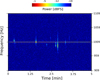 |
Fig. 1 Example of a BRAMS spectrogram recorded for 5 min after processing the signal. The spectrogram displays how the power of the signal is distributed among the frequencies as a function of time. The horizontal line is the direct tropospheric beacon coming from the transmitter. All the vertical traces (we can count up to nine in this plot) are underdense meteor echoes. We give credit to the Royal Belgian Institute for Space Aeronomy. |
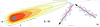 |
Fig. 2 Schematic to describe the methodology pursued in this work. First, the expansion of the metal vapour in the background atmosphere and the consequent hyperthermal collisions are computed using the DSMC-Boltzmann method (i). Second, the long trail evolution is simulated by means of a Lagrangian diffusive reactor marching along the streamlines, which takes advantage of the parabolised nature of the equations. This solver accounts for ionic chemical reactions and radial diffusion (ii). Then, the diffusion coefficient and electron line density are retrieved from the simulations (iii). Finally, the radio echo reflected by an underdense meteor is reconstructed at the receiver (iv). |
2 Methodology
2.1 Phenomenology of the trail
The trail is composed of two regions (see Fig. 3). First, a near trail region, where density and velocity change considerably, and the temperature starts decreasing with respect to the hot ionisation region. This first region, the near trail, is only a few to some hundred diameters long depending on the altitude and entry velocity, and it is entirely out of thermochemical equilibrium. This implies non-Maxwellian distribution functions for the velocity of molecules, and that the gas composition is to be found by finite rate chemistry. Its limited extent allows for the possibility of employing computationally intensive methods, such as DSMC (Boyd 1998; Bariselli et al. 2020) or PIC (Oppenheim & Dimant 2015; Sugar et al. 2018). Nonetheless, due to their statistical nature, tracking minor chemical compounds with such methods could represent a crucial challenge. Therefore, one could wish to thermo-chemically refine the results obtained with these techniques a posteriori.
Second, a far trail region, where the fluid fields (density ρ∞, velocity v∞, and temperature T∞) have reached freestream values. Diffusion processes in the near trail cause strong shear forces and heat exchange between the hot and high-velocity trail and the surrounding fluid at rest, such that fluid dynamic quantities soon reach equilibrium. This denotes the beginning of the far trail, which however remains highly out of equilibrium from the chemical point of view: in contrast with fluid quantities, chemistry is governed by collisions, which are rare in the high atmosphere. This region develops up to several kilometres (therefore, a few tenths of a second in the laboratory frame), and its evolution is governed by mass diffusion of chemical components and chemical reactions. As opposed to the near trail, this region is too extended to be simulated by computationally intensive methods such as DSMC or PIC, and a more computationally efficient methodology must be applied.
2.2 Working assumptions
In order to simplify the treatment of the problem, we have made a series of assumptions. We list them so that the range of validity of our simulations is clarified.
First of all, the body does not fragment, and we assume a two-dimensional steady axisymmetric configuration. Therefore, shear winds that could deform the plasma column and generate multiple reflection points are not considered (McIntosh 1969; Hajduk et al. 1989).
Only molecular diffusion is modelled, while turbulent diffusion, whose scales are of the order of 300 m, is not included. For a numerical study of the effects of turbulence in the trail, the reader can see the work by Oppenheim & Dimant (2015). Also, the effect of the geomagnetic field on the diffusion process is not taken into account. However, the Earth’s magnetic field can lead to anisotropies in the transport properties. This results in a distortion of the trail cross section into an elliptical shape (Jones 1991; Robson 2001; Dimant & Oppenheim 2006). Ions are dominated by collisions up to 140 km, whereas electrons become already magnetised at 80 km (Baggaley 2002).
Ozone concentration is kept constant. However, O3 densities vary significantly between night and day, and this can substantially influence the decay time of the radio signal. The impact of atmospheric ozone was analysed by Baggaley & Cummack (1974).
Finally, free electron temperature is considered in equilibrium with heavy species. However, in general, the electrons cool less rapidly than the ions1. If the thermalisation process usually takes several tens of milliseconds for ions, according to Baggaley & Webb (1977), the electron cooling time varies from about 10−3 s at an altitude of 80 km to about 10−1 s at 115 km.
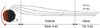 |
Fig. 3 Regions composing the meteor trail. The near trail is only a few hundreds diameters long. The far trail has reached freestream values, but it is still in chemical nonequilibrium and can be several kilometres long. The drawing is not to scale. |
2.3 Governing equations
The Boltzmann equation provides the model which characterises the dynamics of dilute gases, both in and out of thermodynamic equilibrium (Ferziger & Kaper 1972). This equation describes the evolution in time of a probability distribution function fi (x, ξ, t) for each species i over the velocity and physical space. Such a model holds for every rarefaction condition and constitutes a proper framework for an accurate description of the meteor phenomenon (Bariselli et al. 2018). The particle-based DSMC method provides an accurate numerical solution to this equation (Bird 1994).
The link between the distribution function and macroscopic variables can be established by averaging microscopic quantities weighted by fi over the velocity space ξ. By computing the moments of the Boltzmann equation, one can always write a set of species mass, momentum, and energy balances for a reacting flow at the macroscopic level. Considering one mass equation for each species and two other equations for the momentum and energy of the whole mixture, one obtains the so-called Maxwell transfer equations. At steady state these balances read as
 (1)
(1)
 (2)
(2)
 (3)
(3)
where ρi is the density of the i-th species, u the hydrodynamic velocity, and e the mixture thermal energy per unit volume. It is important to note that inter-species friction and energy exchange do not appear, as these terms cancel out at the mixture level. The nonreactive collisional operator has no contribution to Eqs. (1)–(3), since the collisional invariants are in the kernel of this operator (Giovangigli 1999). Therefore, the right-hand side of the Boltzmann equation contributes only to the species mass conservation, through the chemical production rates  , resulting from the reactive collision operator.
Equations (1)–(3) hold independently from the degree of nonequilibrium of the gas (i.e. collisional and collisionless regimes), as long as constitutive relations for the stress tensor Π, heat flux q, and diffusion velocities  are not imposed. In the particular case of asymptotic solution, for small Knudsen numbers (small departures from translational equilibrium), one retrieves the Navier-Stokes equations (Giovangigli 1999).
Diffusive Lagrangian reactor for parabolised equations
We can rework Eqs. (1)–(3), in order to tailor them to the solution of the flow in the trail. First, we can take advantage of a trail property: due to its elongated shape, gradients of fluid and chemical quantities are mainly directed in the radial direction. Since gradients are the main driving forces for mass and energy diffusion processes, this implies that radial diffusion dominates over streamwise diffusion, which can be disregarded.
Second, we can assume that chemistry is partially decoupled from the velocity field in the trail. The idea is that the mixture velocity anddensity obtained with a chemical model are not significantly influenced by the detailed chemistry of minor species, which can be added a posteriori into the problem. This thermo-chemical refinement approach was verified in several test cases by the authors (Boccelli et al. 2019).
Therefore, if velocity and density are given, then the set of mass and energy equations can be solved marching along such precomputed fields, with the initial species concentration and temperature picked from the beginning of the streamlines. In this sense, such precomputed fluid elements resemble a collection of variable volume chemical reactors (see Fig. 4 for a graphical representation).
To do so, Eqs. (1)–(3) are recast into Lagrangian form. This implies reshaping the equations to allow to emerge the material derivative: u⋅∇≡ Ud∕ds, where s is the streamline curvilinear abscissa. After introducing the mass fractions Yi = ρi∕ρ, the mass Eq. (1) of the ith species reads
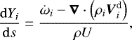 (4)
(4)
where U is the hydrodynamic velocity module. A larger set of species with a more complete chemical mechanism is usually considered for the Lagrangian reactor.
The same procedure can be applied to the energy balance from which an equation for the temperature T is obtained
![\begin{equation*} \frac{\mathrm{d} T}{\mathrm{d} s} = \left[ \mathcal{Q} - \frac{1}{2}\frac{\mathrm{d} U^2}{\mathrm{d} s} - \sum_{i \in \mathcal{S}} h_i \frac{\mathrm{d} Y_i}{\mathrm{d} s} \right]\Biggm/ \left[ \sum_{i \in \mathcal{S}} Y_i c_{\textrm{p}_{i}} \right],\end{equation*}](/articles/aa/full_html/2020/09/aa37454-20/aa37454-20-eq8.png) (5)
(5)
where h is the enthalpy, cp the specific heat, and  the variation of total enthalpy along the streamline which can be expressed, neglecting viscous stresses, as
  , and it is detailed later on.
We note that since the velocity is given, there is no need to solve for the momentum Eq. (2). Besides, since the density comes directly from the velocity field through the mass equation, solving for the global mass equation is not necessary, and it is sufficient to import the assigned density.
Finally, once the density, velocity, and temperature fields have relaxed to freestream conditions (ρ∞, u∞, T∞) in the far trail,the mass balances (Eq. (4)) are the main actors driving the trail evolution through radial gradients in the chemical concentrations. The importance of the energy balance (Eq. (5)) is marginal as the temperature is nearly uniform. The weight of this equation in the far trail lies in the diffusion of the energy produced or absorbed by chemical reactions.
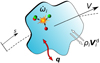 |
Fig. 4 Cartoon of a Lagrangian fluid reactor marching along precomputed streamlines. Species concentrations and energy can evolve inside the reactor because of chemical processes and radial diffusion exchange among different fluid elements. |
2.4 Physico-chemical models
Thermodynamics
Equation (5) requires the evaluation of the species enthalpy hi. Thermodynamic properties can be obtained by means of statistical mechanics, assuming that the energy modes follow a Maxwell-Boltzmann distribution at temperature T (Anderson 2000).
At temperatures close to freestream values, such as the one characterising the far trail, only the contribution of the translational and rotational degrees of freedom of the molecules shall be considered, as the vibrational and electronic modes are not excited2. Moreover, for a chemically reacting flow, the input of the formation enthalpy h0 should also be accounted for. Quantity hi for the i-th species reads as follows
 (6)
(6)
where  for atoms and free electrons and
  for linear molecules, kB and μi being respectively the Boltzmann constant and the mass of the species.
Hydrodynamic closure for mass and energy diffusion fluxes
Despite the high degree of rarefaction, the flow eventually thermalises as the trail develops. This aspect has been studied by different authors (Baggaley & Webb 1977; Boyd 1998; Bariselli et al. 2018). This property allows us to employ near-equilibrium diffusion models based on gradients of thermodynamic quantities, such as the Fourier law and hydrodynamic mass diffusion.
For the quasi-Maxwellian trail, the expressions of the diffusive fluxes  and q can be obtained from the Chapman-Enskog theory (Giovangigli 1999). Diffusion velocities are written as a linear combination of the gradients of species concentration Xi, through the multicomponent diffusion matrix Dij
![\begin{equation*}\boldsymbol{V}_i^{\textrm{d}} = - \sum_{j \in \mathcal{S}} D_{ij} \ \Bigg[ \boldsymbol{\nabla} X_j - \frac{X_j q_j}{k_{\textrm{B}} T} \boldsymbol{E} \Bigg] \ \ \ \ i \in \mathcal{S}, \end{equation*}](/articles/aa/full_html/2020/09/aa37454-20/aa37454-20-eq15.png) (7)
(7)
where the a priori unknown ambipolar electric field E acts as a restoring force to charge neutrality, and it is obtained by constraining the net electric current to zero
 (8)
(8)
qi being the charge and ni the number density of the i-th species3. Thermal and barodiffusion effects are neglected in this work. Heat fluxes include conduction, modelled with the Fourier law, and diffusion of enthalpy
 (10)
(10)
where the temperature gradients ∇T and the heat conduction coefficient λ appear. Diffusion velocities transport the species enthalpy hi.
Finally, the transport coefficients Dij and λ, which appear in Eqs. (7) and (10), require the evaluation of the collision integrals resulting from the Chapman-Enskog solution procedure (Giovangigli 1999). These integrals link interatomic forces at the microscopic level to transport properties at the macroscopic scale. The choice of the potential depends on the nature of the interaction between two species in a given mixture (Capitelli et al. 2000; Bruno et al. 2010; Levin & Wright 2004), as is detailed in Sect. 3.
Chemical kinetics
Metal atoms, M, are produced during ablation, and they ionise as a result of the highly energetic collisions with the atmospheric molecules of the incoming stream (Dressler & Murad 2001). The chemical evolution of these ions influences the radio signal decay, at timescales which can be comparable with those of the diffusion process. In particular, the formation of metal oxide ions (MO+ and MO ) and clusters (M+ ⋅N2), by means of exchange reactions with the background atmosphere, regulate the free electron densities as they are efficiently depleted by fast dissociative recombination reactions (Plane et al. 2015).
If we consider a system of elementary reactions  , we can write
 (11)
(11)
where Xi is the chemical symbol for species  , and
, and  and
and  , the forward and backward stoichiometric coefficients for species i in reaction r. Then, the mass production rate for the i-th chemical component,
  , can be expressed through the law of mass action (Anderson 2000), as follows
![\begin{equation*} \dot{\omega}_i = M_i\sum_{r \in \mathcal{R}} \nu_{ir} \Bigg[ k_{\textrm{f}}\prod_{i \in \mathcal{S}}\left(\frac{\rho_i}{M_i}\right)^{\nu{'}_{ir}} - k_{\textrm{b}}\prod_{i \in \mathcal{S}}\left(\frac{\rho_i}{M_i}\right)^{\nu{''}_{ir}} \Bigg],\end{equation*}](/articles/aa/full_html/2020/09/aa37454-20/aa37454-20-eq25.png) (12)
(12)
where  and symbol Mi stands for the species molar mass. The forward rate coefficients in Arrhenius form reads as
 (13)
(13)
in which therate constants A, η, and Ea are usually determined experimentally. Backward rates, kb, are computed from detailed balance, starting from the available forward rate coefficients and equilibrium constants based on thermodynamic properties.
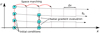 |
Fig. 5 Schematic of the LARSEN numerical procedure along multiple streamlines. |
2.5 An additional note on the Lagrangian reactor
The Lagrangian reactor procedure that we have just introduced can be used for both the near and the far trail. In the first case, velocity anddensity fields are taken from a baseline simulation, to refine the chemical evolution of the ablated vapour by adding more detailed processes. In this region, exchange reactions leading to the formation of metal oxide ions and clusters may start playing a role already (Dressler & Murad 2001), and an accurate description of the chemical mechanism would require a large number of species to be described, most of which are present only as traces. Chemical traces constitute a formidable challenge to DSMC and PIC simulations, as minor species suffer from very large statistical scatter (Hadjiconstantinou et al. 2003). The approach of refining a DSMC baseline simulation, introducing detailed chemistry a posteriori, in the hypothesis that this influences the flowfield only marginally, has shown to provide reliable results in the past (Boccelli et al. 2019), where a near trail DSMC computation was used as a baseline solution, and its chemistry was refined by the Lagrangian reactor method.
Regarding the far trail, velocity and density fields are constant and uniform as they have attained freestream values. Therefore, the streamlines do not vary any more and can be arbitrarily extended up to any length of interest, and these can be used as an input to the diffusive Lagrangian reactor.
In this work, we present results concerning the far trail only. We perform a DSMC simulation of the near trail, and the conditions at the end of the domain are used as initial conditions for the Lagrangian reactor computation.
3 Numerical tools and dataset
3.1 The LARSEN code
At every position along the trail, Eqs. (4) and (5) are discretised radially using a finite volumes scheme (Boccelli et al. 2019) (see Fig. 5). Therefore, at a given timestep, gradients of species concentration and temperature are evaluated. We note that, as each streamline can have different velocity, synchronisation would quickly be lost during the integration, posing an issue to the evaluation of transverse diffusion terms. In order to circumvent this problem, the streamwise derivatives d ∕d sk along each streamline k are converted into derivatives along the symmetry axis x, by taking into account the local streamline slope θk
 (14)
(14)
Once the radial discretisation is performed, the problem has become a system of ODEs in the only variable x, which is integrated using Rosenbrock-4 or Runge-Kutta schemes. Error estimation in the integrator allows the employment of an adaptive step.
The computational cost scales with the number of streamlines considered and depends on the number of species employed, the stiffness of the chemical mechanism, and the characteristic timescales for mass and energy diffusion processes. Overall, the Lagrangian procedure ishighly efficient if compared to the DSMC computation of a trail. Typical simulation time for a 1 km trail is of the order of 20 min on a single-core laptop, while it would easily exceed a few weeks of computation time on several cores for the DSMC method. An implementation of the LAgrangian Reactor for StrEams in Nonequilibrium (LARSEN) code is freely available online4, and more recent versions are available upon request to the authors.
3.2 The MUTATION++ library
The MUTATION++ library (MUlticomponent Thermodynamic And Transport Properties for IoNized plasmas) (Scoggins & Magin 2014) provides thermodynamic, transport, and kinetic models and data to the LARSEN code for the closure of Eqs. (4) and (5). This library is available online5.
The library computes the diffusion velocities and the ambipolar electric field by solving the Stefan-Maxwell system (Magin & Degrez 2004). Transport coefficients for neutral-neutral interactions are derived according to Lennard-Jones (12-6) data available in Svehla (1962), McGee et al. (1998) and Capitelli et al. (2000). Combination rules for those polyatomic species (André et al. 2010), whose potential parameters are not available in the literature, are used. We employ the screened Coulomb (Debye-Hückel) potential shielded at the Debye length for charged-charged collisions. In terms of data, the evaluation of this potential only requires the mass and charge of the colliding species. Concerning ion-neutral interactions, a combination of the Tang-Toennies potential and the Langevin polarisation potential is used, respectively for air-air and metal-air collisions. In particular, air-air collision integrals are taken from the work of Levin & Wright (2004), whereas metal-air collisions are based on the Langevin potential, which necessitates polarisability parameters of the neutral species and the mass of the ion.
Finally, we employ the forward rate coefficients given by Park et al. (2001) for air reactions and the one from Plane et al. (2015) for the thermalised chemical kinetics of metals. A brief review of the latter is given below.
Chemical mechanism for the neutralising trail
The chemistry in the thermalised trail has been widely studied, and the recombination of the metal ions is relatively well understood (Baggaley & Cummack 1974; Baggaley 1978). The interested reader can consult the comprehensive review by Plane et al. (2015) on the topic, where both theoretical and experimental works are reported.
The ablated vapour of an ordinary chondrite mostly comprises iron, magnesium, sodium, and silicon species. In particular, an essential contribution to the production of ions is given by Na, because of its volatile nature and low ionisation potential. Species such as SiO2 and SiO are present in relevant concentrations, contrary to atomic Si, which is characterised by low vapour pressures. For this reason, Si ionisation and its consequential chemical neutralisation are not considered here.
Magnesium and iron (M = Mg, Fe) oxide ions are formed by means of charge exchange processes with the atmospheric ozone
 (15)
(15)
or, below 80 km, by three-body processes in two steps, such as
 (16)
(16)
The resulting oxide ion is efficiently depleted by the fast dissociative recombination reaction
 (18)
(18)
or, in the case of the iron dioxide ion, by
 (19)
(19)
Furthermore, metal clusters can be created by reactions of the following type
 (20)
(20)
where the atmospheric nitrogen plays the role of third-body in the reaction. Magnesium clusters can recombine through dissociation, similarly to Reaction (18) or, in the case of iron, they recycle back to FeO+.
The neutralisation process of sodium is different from the one of Mg and Fe. Na+ has a complete outer electron configuration and can only form a cluster with N2 in a three-body process of this type
 (21)
(21)
with subsequent recombination
 (22)
(22)
The reaction rates included in the chemical mechanism are reported in Table 1.
Reaction rates included in the chemical mechanism for the neutralising trail.
Simulated freestream conditions.
4 Results
We consider a 1 mm diameter meteoroid, flying at 32 km s−1, and evaporating at a surface temperature equal to 2000 K. This value is chosen in agreement with the results obtained in Bariselli et al. (2020), where the wall temperature is characterised by a plateau not far from the melting condition independently from the initial size and velocity. We examine two detection points, one at H = 80 km and the other at 100 km, which represent typical values for radio detection of meteors. The Knudsen number experienced by the evaporating molecules relative to the freestream (Bronshten 1983) reads as
 (23)
(23)
where Vt is the thermal velocity of the ablated atoms leaving in equilibrium with the wall, and Kn∞ is the Knudsen number based on the freestream mean free path  and the meteoroid diameter
 (24)
(24)
For the presented cases, Knr is between the value of 6 at the altitude of 100 km and the value of 0.3 at the altitude of 80 km, these conditions belonging to the transitional regime (10−1 < Knr < 10). Freestream densities, compositions, and temperatures are an input to our model, and computed according to the Naval Research Laboratory Mass Spectrometer Incoherent Scatter Radar (NRLMSISE-00) empirical atmospheric model developed by Picone et al. (2002) and are reported in Table 2, whereas abundances for ozone gas are roughly estimated according to values reported by Baggaley & Cummack (1974). An ordinary chondrite is assumed, for which we assume the following prototypical mass concentrations: 36% SiO2, 25% MgO, 38% FeO, and 1% Na2O.
4.1 Chemical kinetics of metals in an isothermal reactor
We start investigating the chemical mechanism presented in Sect. 3.2, by studying the evolution of the species of meteoric origin independent from the diffusion process, as if the gas was constrained in an isothermal reactor. Freestream values of density and temperature from Table 2 are employed to set the conditions of the reactor, and the atmospheric background species are kept constant in time. As an initial condition, we consider a quasi-neutral mixture of a metal vapour diluted in air, in which the molar fractions are arbitrarily set as Mg+ = 0.1%, Fe+ = 0.1%, and Na+ = 1.0%.
For magnesium, the formation of oxide ions in trace concentrations, such as MgO+ and  , precedes the actual recombination of the free electrons, as is shown by Fig. 6. In the same figure, the ion chemistry relevant to iron behaves similarly to the one of magnesium, but concentrations of FeO
 are lower, if compared to MgO
 , because the former is directly lost by dissociation via Reaction (19). In Fig. 7, recombination appears to be significantly dependent on the background pressure for both magnesium and iron, mainly because of the influence of Reaction (20) in the deionisation process.
With reference to sodium, the neutralisation mechanism is significantly different and controlled by the cluster  . Since it only relies on three-body collisions (Reaction (21)), it is characterised by longer timescales. This effect is better shown in Fig. 7, where timescales for recombination increase up to three orders of magnitude, moving from 80 to 100 km.
From this analysis, we can conclude that, at an altitude of 80 km, ion chemistry in the trail proceeds at rates which are likely to be comparable with the timescales of mass diffusion. On the other hand, we have to exclude that chemical reactions can play any role in the radio signal decay at 100 km.
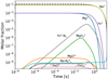 |
Fig. 6 Evolution of the chemicals of meteoric origin involved in the deionisation process in the background atmosphere at an altitude of 80 km. Free electrons are represented with a dashed black line. |
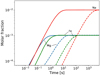 |
Fig. 7 Influence of the atmospheric pressure in the neutralisation of the trail. Comparison between 80 and 100 km altitude. The effect of the background pressure is particularly evident for Na, whose recombination is fully driven by a three-body process. Dashed lines refer to 80 km and solid lines to 100 km. |
4.2 Analysis of the trail
We simulate the full trail with the methodology described in Sect. 2. First, we briefly discuss the main features of the near trail, which are obtained through the SPARTA (Stochastic PArallel Rarefied-gas Time-accurate Analyzer) DSMC-Boltzmann solver by Gallis et al. (2014). This discussion allows us to examine the hypotheses introduced in Sect. 2, with regard to thermal equilibrium, velocity and density fields. In a second step, we employ the information at the outlet of the DSMC domain, and we march along the freestream streamlines with LARSEN, in order to compute the chemistry in the far trail.
It is important to note that all the plots of the trail have to be considered in a frame of reference fixed to the meteoroid. Therefore, the reported simulations are to be interpreted, by a ground-based observer, as simulations of one point of the trajectory. What an observer moving with the meteoroid sees as a trail, which relaxes to the freestream velocity and develops in space, is seen by a ground observer as the radial evolution of a trail, whose velocity relaxes to zero a few diameters after the meteoroid. In this way, the given plots can be interpreted as the radial evolution in one particular position of the sky, as time passes.Freestream density and temperature in the background atmosphere can thus be taken to be constant during the radial evolution, even for extensive simulations. The conversion between the indicated spatial position x and the ground-observer elapsed timet is obtained through the flight velocity U∞ at the reflection point: t = x∕U∞.
SPARTA DSMC-Boltzmann simulations of the near trail
We model the evaporation process of a spherical body and the dynamics of the gas in the axisymmetric near trail using the SPARTA DSMC-Boltzmann code. Evaporation rates are computed according to the equilibrium partial densities provided by the multi-phase multi-species equilibrium solver MAGMA by Fegley & Cameron (1987). Once evaporated, energetic impacts with the incoming air stream lead to the ionisation of metal atoms, as a consequence of processes of this type
 (25)
(25)

Also, air species contribute to the production of free electrons through the mechanism provided by Park et al. (2001) for the NASA Air-11 mixture: N2, O2, N, O, NO, and their ions. The translational-internal energy exchanges are modelled according to the classical phenomenological model by Borgnakke & Larsen (1975). Moreover, we assume that metals are not involved in exchange reactions in the near trail so that metal oxide ions and clusters can only be produced in the far trail. Free electrons, whose diffusion is modelled under the ambipolar assumption, are expected to recombine later in the far trail.
A detailed description of these DSMC simulations is out of the scope of this paper and can be found in Bariselli et al. (2020). On the contrary, we are interested in examining the hypotheses pertinent to the relaxation to freestream conditions and the initial condition profiles which are provided to the far trail simulations.
The dynamics of the gas to the rear of the body can be best appreciated by plotting the development in the physical space of the velocity distribution function (VDF), as is done in Fig. 8, for both the axial and the radial velocities. These distribution functions are obtained by sampling DSMC particles at different stations along the trail, in regions which are one meteoroid diameter in height.
In the near trail (from 0 to roughly 150 diameters in this test case), both the axial and radial VDFs are characterised by a bimodal shape, and the two families of particles, the metal vapour and the air, do not interact significantly. Indeed, thermalisation would push the two VDFs towards a common Maxwellian distribution. Also, Fig. 8 shows that the near trail quicklyassumes the freestream velocity condition as the trail is progressively filled by fast air molecules which, in a few diameters, take over the slow ablated vapour. This process occurs in only a few mean free paths and eventually, even in a low collisionality regime, it leads to a Maxwellian distribution, at the end of the near trail.
The metal vapour diffuses in the surroundings, nearly in thermal equilibrium with the wall, with a law not far from the one describing an expansion into a vacuum (~1∕r2) (see the metal vapour density field in Fig. 9). Moreover, in Fig. 9, we can see how the average density in the near trail region reaches the values of the freestream in nearly 100 diameters. Also, in Fig. 10, similar relaxation times apply to the translational and internal temperatures. Here, translational and rotational degrees of freedom in the near trail take only a few microseconds (around 10 mean free paths) to equilibrate and relax to the values of the freestream, confirming that the importance of Eq. (5) is marginal in the far trail. In the near trail, the very high temperatures observed (up to 105 K) arise from the mixing of the two families of molecules, freestream and ablated vapour. This results in a global population strongly out of equilibrium, and whose dispersion – and therefore temperature – appears extremely high. Rather than the thermal content of the single population, this is to be interpreted as a geometrical temperature.
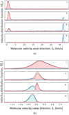 |
Fig. 8 Evolution along the near trail of the axial VDF f(ξx) (a) and the radial VDF f(ξr) (b): (i) x∕D = 0.5 ( |


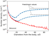 |
Fig. 9 DSMC density profiles along the near trail for the two different altitude conditions, 80 km (marker |


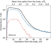 |
Fig. 10 Translational and internal temperature profiles along the near trail at 80 km altitude. The reference system is centred at the stagnation point. In the near trail, Ttr (solid black line) and Trot (dashed blue line) take only a few microseconds (around 10 mean free paths) to relax to the values of the freestream. Vibrational temperature is marked with a dotted red line. |
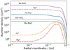 |
Fig. 11 Radial profiles for species densities at the beginning of the far trail domain, at an altitude of 80 km. Profiles are reported after a few steps of integration in LARSEN. This reduces considerably the noise characterising chemical traces simulated inDSMC. |
LARSEN Lagrangian reactor simulations of the far trail
We start the computation of the far trail from the radial profiles obtained at the outlet of the DSMC domain. In Fig. 11, we show these profiles at 80 km after a few steps of integration in LARSEN, which reduces considerably the noise characterising the chemical traces in DSMC.
If we look at the density profiles in Fig. 12, chemical traces of sodium are present far behind the meteoroid. At high altitude, the trail tends to diffuse much more than at lower altitude: at 100 km, metal traces are detectable in a 10 m radius cone after 1 km.
At 80 km, exchange reactions are active and produce metal oxide ions and clusters. For these species, profiles at the axis of symmetry of the simulation domain are plotted in Fig. 13. However, in the next section, we show that their influence is marginal in the dynamics of the free electrons. Indeed, the evolution of radial profiles suggests a deionisation process dominated by diffusion. We give a quantitative evaluation of this in the following section.
Electron line density and ambipolar diffusion coefficient extracted from trail simulations
We can compare the present numerical result with the analytical solution for a problem of pure diffusion. In the case of a dilute solution at constant mixture density, Eq. (1) reduces to
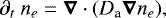 (27)
(27)
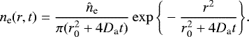
Here, we areassuming that ions and electrons diffuse at the same rate governed by the common and constant ambipolar diffusion coefficient Da. From the electron number density ne, the electron line density  can be directly extracted from the simulations by numerical integration, as follows
 (29)
(29)
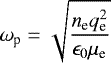
which is constant along the trail (therefore in time), if chemistry is not important. The initial meteor radius r0 is taken equal to the radial width of the DSMC computational domain that is equal to 10 and 40 meteoroid radii respectively at 80 and 100 km6. In this regard, we would like to point out that the employed DSMC domains are probably not large enough to contain the full ionisation profile, as an ablated atom may take several mean free paths before ionising. Therefore, it may be that we are underestimating the total free electron production. For both our simulated conditions, the electron line density turns out to be nearly constant. Its values can be found in Table 3. In Fig. 14, electron density profiles at an altitude of 100 km are seen to follow the analytical solution for radial diffusion closely, once the proper diffusion coefficient is chosen. The close agreement confirms the importance of diffusion over chemistry for the current conditions and the fact that a constant diffusion coefficient represents a fair assumption. Diffusion coefficients are obtained by fitting Eq. (28) over the numerical profiles. The ambipolar diffusion coefficients resulting from LARSEN simulations are reported in Table 3 and show that the trail expands faster at 100 km than 80 km altitude.
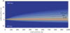 |
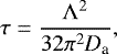
Fig. 12 Ablated vapour expansion in the trail of the meteor. Number density contours at 80 and 100 km altitude show how much faster the vapour expands at higher altitudes. Contours (104, 106, and 1010 1/m3) are drawn for the Na species for both conditions. The freestream flows from left to right. |
 |
Fig. 13 Evolution of the chemicals of meteoric origin involved in the deionisation process, at an altitude of 80 km. Reported values refer to the axis of symmetry. Exchange reactions are active at this condition, but their influence is marginal in predicting the evolution of the electrons. |
Electron line densities and ambipolar diffusion coefficients resulting from the numerical simulations.
4.3 Link of trail simulations to the radio-echo theory
When the density of the free electrons is weak (underdense reflection), the classical theory for wave-plasma interactions (McKinley 1961) assumes that the incident radio wave can propagate in the ionised gas, where it is scattered by the individual electrons with no secondary scattering and absorption effects. On the other hand, when the meteor is overdense, free electrons cannot behave as autonomous reflectors, and the physics of the wave-plasma interaction is more complicated.
The underdense condition can be formally written as ne < ncr (Foschini 1999), where ncr represents the critical density, which is reached when the plasma frequency
 (30)
(30)
attains the value of the impinging radio wave frequency. In Eq. (30), quantity qe represents the electron charge, μe the mass of the electron, and ɛ0 the permittivity of free space.
If we assume a wavelength Λ = 6 m, which corresponds to a radio frequency equal to 50 MHz, the overdense region extends up to 100 m along the axial direction and 5 cm in the radial one at 80 km altitude. The overdense region can be seen in Fig. 15 for the 80 km case. On the other hand, at 100 km, the overdense region appears to be only a few centimetres long, and the underdense condition is fulfilled practically everywhere.
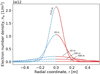 |
Fig. 14 Comparison of the analytical (solid red lines) and numerical solutions (dashed blue lines) for the electron density profiles at different positions in the far trail at 100 km altitude. |
Reconstruction of the underdense radio echo
If underdense plasma theory applies, and the trail is regarded as a scattering cone (Eq. (28)) with a Gaussian density distribution, then an analytical treatment to the signal reconstruction exists (Verbeeck 1995). In the hypothesis of a plasma column dominated by diffusion, classical radio theory for the forward-scattering technique predicts a power delivered to the receiver which reads as
![\begin{align*} P_{\textrm{R}}(t) =&\, \frac{c_0 \Lambda^3 r_{\textrm{e}}^2 \hat{n}_{\textrm{e}}^2}{32 \pi^2 c_1} \ \exp \!\left\{\! \frac{-8 \pi^2 c_2 (r_0^2 + 4D_{\textrm{a}} t) }{\Lambda^2} \!\right\} \times \frac{1}{2} [\mathcal{C}^2(t) + \mathcal{S}^2(t)]\end{align*}](/articles/aa/full_html/2020/09/aa37454-20/aa37454-20-eq51.png) (31)
(31)
for t > 0 s. Constant c0 depends on the apparatus, whereas c1 and c2 depend on the geometry of the detection. Quantities Λ and re are respectively the wavelength of the incident radio wave and the classical radius of the electron. Finally,  and
and  stand for the Fresnel integrals coming from diffraction phenomena.
Given the geometry of the detection (see Fig. 16 for its graphical representation) and the technical parameters of the radio system, we can reconstruct an hypothetical radio echo, using the physical quantities of the plasma extracted from the simulations in Eq. (31). In the BRAMS network (Lamy et al. 2011), a dedicated beacon is installed in Dourbes, Belgium. It emits a continuous waveform circularly polarised signal at a frequency of 49.97 MHz with a constant power PT = 150 W. In Eq. (31), parameter c0 is defined as
 (32)
(32)
γ being the angle between the electric field of the incoming wave and the line of sight of the receiver. For the sake of simplicity, we assume the gains of the transmitter and the receiver, respectively GT and GR, equal to one, and we set sin2γ = 1∕2 (Verbeeck 1995), being γ the angle between the electric field vector of the incoming wave and the line of sight of the receiver.
Constants c1 and c2 fully depend on the geometry of the detection and respectively read as
 (33)
(33)
where RT and RR are the distances of the transmitter and the receiver from the reflection point, ϕ is half of the angle between the transmitter and the receiver at the reflection point, and β the angle between the wave propagation plane, defined by the ellipse in Fig. 16, and the meteor entry trajectory.
We imagine the reflected signal to be received by the BRAMS radio station in Overpelt, Belgium. We set β =0 deg, and weconsider that the wave propagation plane is not inclined with respect to the local normal to the surface. For both conditions, we simulate two different reflection points: one xd = 70 km and the other 117 km away from the transmitter. In Fig. 17, we see that this distance influences the intensity of the signal (roughly by a factor 1∕R3 according toEq. (33)), but not its shape.
At 80 km altitude, the Fresnel oscillations are evident, whereas at 100 km, these fluctuations are significantly damped by the intense diffusion rate. Also, for the first case, the signal lasts up to 0.3 s, a much longer duration with respect to Condition 2, where the echo quickly disappears after 0.025 s. Finally, due to the higher electron densities characterising the plasma column, the intensity of the received power appears to be three orders of magnitude larger for the first case than in the second7.
Comparison of the ambipolar diffusion coefficients with theory and radio/radar decay observations
We can now examine the diffusion coefficients extracted from the numerical simulations in the light of classical theoretical results and radio decay observations. In a three-component thermalised plasma containing neutrals, ions, and electrons, a standard result (Kaiser 1953; Ramshaw & Chang 1993) predicts the ambipolar diffusion coefficient to be
 (35)
(35)
 being the ion-neutral binary diffusion coefficient, with index i and j respectively representing the ion and neutral species. The Einstein’s relation defines binary diffusion coefficients for ions in a neutral gas as
 (36)
(36)
where  is the zero-field mobility factor (Mason & McDaniel 1988). Langevin’s theory of ionic mobilities predicts a dependency of
  on the mass of the ion and the polarisability of the neutral molecule (Massey et al. 1971). This theory has shown general good agreement with meteor decay times (Jones & Jones 1990), and it is consistent with the approach adopted here, where ion-neutral binary diffusion coefficients
  , arising from the Chapman-Enskog method (see Appendix A), are computed using the Langevin potential. A comparison of the binary diffusion coefficients employed in this work with results obtained by means of Eq. (36) and zero-field mobilities by Massey et al. (1971) is given in Fig. 18, for some relevant ions diffusing in N2. A difference exists in the data of N+ and O+, for which more accurate data have been used (Levin & Wright 2004). Also, ambipolar diffusion rates extracted from the simulations and reported in Table 3 are coherent with those predicted combining Eqs. (35) and (36), if we consider that Na+ and Mg+ are the most abundant ions in the simulations.
Finally, we compare results from our numerical simulations with observations. Astronomers have proposed a variety of observational fittings to obtain the ambipolar diffusion coefficient from the exponential decay constant, which is given by
 (37)
(37)
and it is computed as the time that the echo intensity takes to decay by a factor 1∕e (Herlofson 1947). In Fig. 19, we consider some of these fits (Greenhow & Hall 1961; Jones & Jones 1990; Galligan et al. 2004). We also report the data collected by the Advanced Meteor Orbit Radar (AMOR) (Baggaley et al. 2002), over which the fitting by Galligan et al. (2004) is based. Contour lines correspond to the number of detections. We find the diffusion of free electrons to be in good agreement with the ones retrieved by observations, even if simulations seems to slightly overpredict diffusion coefficients. Although scatters in the experimental data suggest caution in the comparison, possible reasons for this discrepancy could reside in the differences among the employed atmospheric models, in the inhibition of diffusion by the geomagnetic field (Cervera & Reid 2000), or in overestimated concentrations of Na+ in the simulations, with respect to Mg+ and Fe+. The far trail is computed in all its length, assuming a frozen composition of the meteoroid equal to its initial condition. However, a depletion in volatile elements in the first part of the entry path would lower sodium concentrations, and the vapour phase would start being dominated by refractory elements (McNeil et al. 1998; Janches et al. 2009).
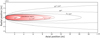 |
Fig. 15 Contour plot of the electron number density for Condition 1, at 80 km altitude. The overdense region is highlighted. We have assumed a wavelength Λ = 6 m, which corresponds to a radio frequency equal to 50 MHz. For this condition, the region extends up to 100 m in the axial direction and 5 cm in the radial direction. Axes are not to scale and the freestream flows from left to right. |
 |
Fig. 16 (a) Graphical representation of the radio signal forward-scattered by a meteor trail. The optical path of the reflection is specular. Reflections of the emitted signal from other segments of the trail can result in diffraction patterns, which are accounted in Eq. (31) by the Fresnel integrals. (b) Two hypothetical detection points for Condition 1 and 2. The transmitter in Dourbes, Belgium emits a continuous radio wave at a frequency of 49.97 MHz and constant power of 150 W. The reflected signal is received by the radio station in Overpelt, Belgium. The ellipse defines the wave propagation plane, and the two entry trajectories are tangential to the ellipse at the reflection points. Moreover, we assume that the trajectories lie in the plane of propagation of the wave, having set β = 0 deg. |
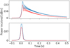 |
Fig. 17 Simulated power profiles for Condition 1 (upper) and Condition 2 (lower). At t = 0 s, the meteor is at the reflection point. For both conditions, we simulate two different reflection points: one 70 km (solid blue lines) and the other 117 km (dashed red lines) away from the transmitter. Here, we are assuming that the wave propagation plane is not inclined with respect to the local normal to the surface. |
 |
Fig. 18 Binary diffusion coefficients for some relevant ion-N2 collision pairs for Condition 1 (upper) and Condition 2 (lower). Marker |


5 Conclusions
We have introduced a method to model meteor plasma trails up to several kilometres in length, under rarefied conditions. This method is a general and self-consistent procedure that allows the computation of meteor physical parameters at given trajectory conditions, without the need to rely on phenomenological lumped models. In particular, we have analysed the main physico-chemical features of the near and far trail, and we have retrieved diffusion coefficient and electron line density, parameters of vital importance for the interpretation of radio- scattering.
As test case, we have investigated the formation and development of the trail generated by a 1 mm ordinary chondrite, flying at 32 km s−1, at altitudes of 80 and 100 km. Starting from DSMC computations of the evaporating meteoroid, and the following ionisation reactions, we have calculated the multicomponent diffusion, ambipolar electric field, and chemistry relevant to the dissipation of the plasma trail. In the near trail, translational and rotational degrees of freedom of heavy species take only a few microseconds to relax to the values of the freestream. In the far trail, ionic chemical reactions, although active, have shown not to play a significant role in the neutralisation process, which is dominated by mass diffusion. Also, a common and constant diffusion coefficient was sufficient to reproduce the numerical profiles. The influence of chemistry and differential radial diffusion could be enhanced in overdense meteors, therefore this aspect deserves further investigation. Moreover, the extracted ambipolar diffusion coefficients have been compared with theoretical values and observations, finding a good agreement in both cases. As a last step, we have linked the dissipation of the free electrons in the trail to the classical radio-echo theory of underdense meteors, verifying whether applying this condition is legitimate or not for the tested conditions.
In a future perspective, it is desirable to examine the methodology against radio observations in order to compare experimental echoes with the ones synthetically generated through simulations. This procedure would provide validation of the models and further insight into the phenomena involved. Finally, the electron fields obtained numerically open the possibility of employing more sophisticated methods to study more in detail the interaction of the plasma with the electromagnetic wave, for instance Finite-Difference Time-Domain (FDTD) (Marshall & Close 2015), optical ray tracing (Vecchi et al. 2004), or Volume-Surface Integral Equation (VSIE) (Sha et al. 2019) techniques.
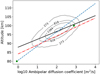 |
Fig. 19 Base-10 logarithm of the ambipolar diffusion coefficient in function of the altitude. Comparison between numerical simulations from present work (marker |

Acknowledgements
The authors thank Dr Cis Verbeeck, research scientist at the Royal Observatory of Belgium, for providing the code used to compute the power profile of a forward-scattered radio wave. We also acknowledge Dr Hervé Lamy, research scientist at the Royal Belgian Institute for Space Aeronomy, for sharing with us the BRAMS spectrogram. The research of FB is funded by a PhD grant of the Research Foundation Flanders (FWO) and the one of BD by a PhD grant of the Funds for Research Training in Industry and Agriculture (FRIA).
Appendix A Diffusion coefficients and interatomic potentials in MUTATION++
The diffusion velocities are solution of the Stefan-Maxwell system that requires the evaluation of the binary diffusion coefficients  . Details on this system and on its efficient solution can be found in the work of Magin & Degrez (2004). Between species i and j, a coefficient reads as
 (A.1)
(A.1)
where  is the reduced mass and
  the collision integral, defined as
 (A.2)
(A.2)
Here, variable b is the impact parameter characterising the binary collision and  a reduced variable for the relative velocity gij. The scattering angle, χ = χ(b, g, ψ), resulting from the dynamic of the binary collision, directly depends on the relevant interatomic potential, ψ.
For neutral-neutral collisions, we employ the Lennard-Jones (12-6) potential
![\begin{equation*} \psi_{ij}(r) = 4\epsilon_{ij} \Bigg[\Bigg(\frac{\bar{\sigma}_{ij}}{r}\Bigg)^{12} - \Bigg(\frac{\bar{\sigma}_{ij}}{r}\Bigg)^6 \Bigg],\end{equation*}](/articles/aa/full_html/2020/09/aa37454-20/aa37454-20-eq70.png) (A.3)
(A.3)
where quantity ɛij is the depth of the potential well,  is the finite distance at which thepotential is zero, and r is the distance between the particles. Charged-charged interactions are treated according to the screened Coulomb (Debye-Hückel) potential
 (A.4)
(A.4)
where z the elementary charge and λD the Debye length that reads as
 (A.5)
(A.5)
Finally, for neutral-ion interactions, where i is the neutral and j the charged species, we use the Langevin polarisation potential
 (A.6)
(A.6)
where αi is the dipole polarisability of the neutral species.
References
- Anderson, J. D. 2000, Hypersonic and High Temperature Gas Dynamics (UAS: AIAA) [Google Scholar]
- André, P., Aubreton, J., Clain, S., et al. 2010, Euro. Phys. J. D, 57, 227 [CrossRef] [EDP Sciences] [Google Scholar]
- Baggaley, W. J. 1978, Planet. Space Sci., 26, 979 [CrossRef] [Google Scholar]
- Baggaley, W. J. 2002, Radar observations in Meteors in the Earth’s Atmosphere, eds. E. Murad, & I. P. Williams, (Cambridge: Cambridge University Press) [Google Scholar]
- Baggaley, W. J., & Cummack, C. H. 1974, J. Atmos. Terr. Phys., 36, 1759 [CrossRef] [Google Scholar]
- Baggaley, W. J., & Webb, T. H. 1977, J. Atmos. Terr. Phys., 39, 1399 [CrossRef] [Google Scholar]
- Baggaley, W. J., Bennett, R. G. T., Marsh, S. H., Plank, G. E., & Galligan, D. P. 2002, COSPAR Colloquia Series: Dust in the Solar System and other Planetary Systems (Amsterdam: Elsevier), 15, 38 [Google Scholar]
- Bariselli, F., Boccelli, S., Frezzotti, A., Hubin, A., & Magin, T. E. 2018, AIAA Conference Proceedings, AIAA 2018-4180 [Google Scholar]
- Bariselli, F., Frezzotti, A., Hubin, A., & Magin, T. E. 2020, MNRAS, 492, 2308 [NASA ADS] [CrossRef] [Google Scholar]
- Bird, G. A. 1994, Molecular Gas Dynamics and the Direct Simulation of Gas Flows (Oxford: Oxford University Press) [Google Scholar]
- Boccelli, S., Bariselli, F., Dias, B., & Magin, T. E. 2019, Plasma Sources Sci. Technol., 28, 065002 [CrossRef] [Google Scholar]
- Borgnakke, C., & Larsen, P. S. 1975, J. Comput. Phys., 18, 405 [CrossRef] [Google Scholar]
- Boyd, I. D. 1998, Earth Moon Planets, 82, 93 [CrossRef] [Google Scholar]
- Bronshten, V. A. 1983, Physics of Meteoric Phenomena (Boston: D. Reidel Publishing Co.) [CrossRef] [Google Scholar]
- Bruno, D., Catalfamo, C., Capitelli, M., et al. 2010, Phys. Plasmas, 17, 112315 [NASA ADS] [CrossRef] [Google Scholar]
- Capitelli, M., Gorse, C., Longo, S., & Giordano, D. 2000, J. Thermophys. Heat Transf., 14, 259 [CrossRef] [Google Scholar]
- Ceplecha, Z., Borovička, J., Elford, W. G., et al. 1998, Space Sci. Rev., 84, 327 [NASA ADS] [CrossRef] [Google Scholar]
- Cervera, M. A., & Reid, I. M. 2000, Rad. Sci., 35, 833 [CrossRef] [Google Scholar]
- Dimant, Y. S., & Oppenheim, M. M. 2006, J. Geophys. Res. Space Phys., 111, A12 [Google Scholar]
- Dressler, R. A., & Murad, E. 2001, in Chemical Dynamics in Extreme Environments, ed. Dressler, R. A. (Singapore: World Scientific) [CrossRef] [Google Scholar]
- Fegley, B., & Cameron, A. G. W. 1987, Earth Planet. Sci. Lett., 82, 207 [NASA ADS] [CrossRef] [Google Scholar]
- Feng, W., Marsh, D. R., Chipperfield, M. P., et al. 2013, J. Geophys. Res. Atmos., 118, 9456 [CrossRef] [Google Scholar]
- Ferziger, J. H., & Kaper, H. G. 1972, Mathematical Theory of Transport Processes in Gases (Amsterdam: Elsevier Science Publishing) [Google Scholar]
- Forsyth, P. A., & Vogan, E. L. 1955, Can. J. Phys., 33, 176 [CrossRef] [Google Scholar]
- Foschini, L. 1999, A&A, 341, 634 [NASA ADS] [Google Scholar]
- Galligan, D. P., Thomas, G. E., & Baggaley, W. J. 2004, J. Atmos. Sol.-Terr. Phys., 66, 899 [CrossRef] [Google Scholar]
- Gallis, M. A., Torczynski, J. R., Plimpton, S. J., Rader, D. J., & Koehler, T. 2014, AIP Conf. Proc., 1628, 27 [CrossRef] [Google Scholar]
- Giovangigli, V. 1999, Multicomponent Flow Modeling. Modeling and Simulation in Science, Engineering and Technology (Boston, MA: Birkähuser Boston Inc.) [CrossRef] [Google Scholar]
- Greenhow, J. S., & Hall, J. E. 1961, Planet. Space Sci., 5, 109 [CrossRef] [Google Scholar]
- Hadjiconstantinou, N. G., Garcia, A. L., Bazant, M. Z., & He, G. 2003, J. Comput. Phys., 187, 274 [CrossRef] [MathSciNet] [Google Scholar]
- Hajduk, A., Stohl, J., & Cevolani, G. 1989, Nuovo Cimento, 12, 315 [CrossRef] [Google Scholar]
- Herlofson, N. 1947, Rep. Prog. Phys., 11, 444 [Google Scholar]
- Hocking, W. K., Fuller, B., & Vandepeer, B. 2001, J. Atmos. Sol.-Terr. Phys., 63, 155 [CrossRef] [Google Scholar]
- Hocking, W. K., Thayaparan, T., & Jones, J. 1997, Geophys. Res. Lett., 24, 2977 [CrossRef] [Google Scholar]
- Janches, D., Dyrud, L. P., Broadley, S. L., & Plane, J. M. C. 2009, Geophys. Res. Lett., 36, 6 [Google Scholar]
- Jones, W. 1991, Planet. Space Sci., 39, 1283 [CrossRef] [Google Scholar]
- Jones, W. 1997, MNRAS, 288, 995 [NASA ADS] [CrossRef] [Google Scholar]
- Jones, W., & Jones, J. 1990, J. Atmos. Terr. Phys., 52, 185 [CrossRef] [Google Scholar]
- Kaiser, T. R. 1953, Adv. Phys., 2, 495 [CrossRef] [Google Scholar]
- Lamy, H., Ranvier, S., Keyser, J., Gamby, E., & Calders, S. 2011, Meteoroids Conference Proceedings, NASA/CP–2011–216469, 351 [Google Scholar]
- Levin, E., & Wright, M. J. 2004, J. Thermophys. Heat Transf., 18, 143 [CrossRef] [Google Scholar]
- Magin, T. E., & Degrez, G. 2004, J. Comput. Phys., 198, 424 [NASA ADS] [CrossRef] [Google Scholar]
- Marshall, R. A., & Close, S. 2015, J. Geophys. Res. Space Phys., 120, 5931 [CrossRef] [Google Scholar]
- Mason, E. A.,& McDaniel, E. W. 1988, Transport Properties of Ions in Gases (Hoboken: John Wiley & Sons) [CrossRef] [Google Scholar]
- Massey, H. S. W., Burhop, E. H. S., & Gilbody, H. B. 1971, Electronic and Ionic Impact Phenomena (Oxford: Clarendon Press), 3 [Google Scholar]
- McGee, B. C., Hobbs, M. L., & Baer, M. R. 1998, Exponential 6 Parameterization for the JCZ3-EOS, Tech. rep., Sandia National Labs., Albuquerque, NM, SAND98-1191 [Google Scholar]
- McIntosh, B. A. 1969, Can. J. Phys., 47, 1337 [CrossRef] [Google Scholar]
- McKinley, D. W. R. 1961, Meteor Science and Engineering (New York: McGraw-Hill) [Google Scholar]
- McNeil, W. J., Lai, S. T., & Murad, E. 1998, J. Geophys. Res. Atmos.., 103, 10899 [CrossRef] [Google Scholar]
- Oppenheim, M. M., & Dimant, Y. S. 2015, Geophys. Res. Lett., 42, 681 [CrossRef] [Google Scholar]
- Park, C., Jaffe, R. L., & Partridge, H. 2001, J. Thermophys. Heat Transf., 15, 76 [CrossRef] [Google Scholar]
- Picone, J. M., Hedin, A. E., Drob, D. P., & Aikin, A. C. 2002, J. Geophys. Res. Space Phys., 107, 15 [Google Scholar]
- Plane, J. M. C. 2004, Atmos. Chem. Phys., 4, 627 [NASA ADS] [CrossRef] [Google Scholar]
- Plane, J. M. C., & Whalley, C. L. 2012, J. Phys. Chem. A, 116, 6240 [CrossRef] [Google Scholar]
- Plane, J. M. C., Feng, W., & Dawkins, E. C. M. 2015, Chem. Rev., 115, 4497 [CrossRef] [Google Scholar]
- Ramshaw, J. D., & Chang, C. H. 1993, Plasma Chem. Plasma Process., 13, 489 [CrossRef] [Google Scholar]
- Robson, R. 2001, Phys. Rev. E, 63, 026404 [CrossRef] [Google Scholar]
- Scoggins, J. B., & Magin, T. E. 2014, 11th AIAA/ASME Joint Thermophysics and Heat Transfer Conference, AIAA 2014-2966 [Google Scholar]
- Sha, Y., Zhang, H., Guo, X., & Xia, M. 2019, IEEE Transac. Antennas Propag., 67, 2470 [CrossRef] [Google Scholar]
- Sugar, G., Oppenheim, M. M., Dimant, Y. S., & Close, S. 2018, J. Geophys. Res. Space Phys., 123, 4080 [CrossRef] [Google Scholar]
- Svehla, R. A. 1962, Estimated viscosities and thermal conductivities of gases at high temperatures, Tech. rep., NASA Lewis Research Center, Cleveland, OH, NASA-TR-R-132 [Google Scholar]
- Vecchi, C., Sabbadini, M., Maggiora, R., & Siciliano, A. 2004, IEEE Antennas Propag. Soc. Symp., 1, 181 [CrossRef] [Google Scholar]
- Verbeeck, C. 1995, 14th International Meteor Conference, Brandenburg, Germany, 83 [Google Scholar]
- Weryk, R. J., & Brown, P. G. 2013, Planet. Space Sci., 81, 32 [NASA ADS] [CrossRef] [Google Scholar]
- Zinn, J., Judd, O. P., & Revelle, D. O. 2004, Adv. Space Res., 33, 1466 [NASA ADS] [CrossRef] [Google Scholar]
We note that in this general formulation, the effects of the ambipolar electric field do not rely on the definition of an ambipolar diffusion coefficient. The ambipolar electric field can be promptly evaluated a posteriori in the form
 (9) by imposing zero net electric current. The multicomponent ambipolar matrix is retrieved by substituting the obtained electric field in Eq. (7).
The literature refers to the initial meteor radius as the span of the cylinder of ionised plasma that is quasi-instantaneously formed upon the passage of the meteoroid. In a consistent way, we are implying that only the processes occurring in the near trail can be responsible for the production of free electrons. Consequently, we define the initial meteor radius according to the ionisation profile developed at the outlet of the DSMC computational domain.
All Tables
Electron line densities and ambipolar diffusion coefficients resulting from the numerical simulations.
All Figures
|
Fig. 1 Example of a BRAMS spectrogram recorded for 5 min after processing the signal. The spectrogram displays how the power of the signal is distributed among the frequencies as a function of time. The horizontal line is the direct tropospheric beacon coming from the transmitter. All the vertical traces (we can count up to nine in this plot) are underdense meteor echoes. We give credit to the Royal Belgian Institute for Space Aeronomy. |
| In the text | |
|
Fig. 2 Schematic to describe the methodology pursued in this work. First, the expansion of the metal vapour in the background atmosphere and the consequent hyperthermal collisions are computed using the DSMC-Boltzmann method (i). Second, the long trail evolution is simulated by means of a Lagrangian diffusive reactor marching along the streamlines, which takes advantage of the parabolised nature of the equations. This solver accounts for ionic chemical reactions and radial diffusion (ii). Then, the diffusion coefficient and electron line density are retrieved from the simulations (iii). Finally, the radio echo reflected by an underdense meteor is reconstructed at the receiver (iv). |
| In the text | |
|
Fig. 3 Regions composing the meteor trail. The near trail is only a few hundreds diameters long. The far trail has reached freestream values, but it is still in chemical nonequilibrium and can be several kilometres long. The drawing is not to scale. |
| In the text | |
|
Fig. 4 Cartoon of a Lagrangian fluid reactor marching along precomputed streamlines. Species concentrations and energy can evolve inside the reactor because of chemical processes and radial diffusion exchange among different fluid elements. |
| In the text | |
|
Fig. 5 Schematic of the LARSEN numerical procedure along multiple streamlines. |
| In the text | |
|
Fig. 6 Evolution of the chemicals of meteoric origin involved in the deionisation process in the background atmosphere at an altitude of 80 km. Free electrons are represented with a dashed black line. |
| In the text | |
|
Fig. 7 Influence of the atmospheric pressure in the neutralisation of the trail. Comparison between 80 and 100 km altitude. The effect of the background pressure is particularly evident for Na, whose recombination is fully driven by a three-body process. Dashed lines refer to 80 km and solid lines to 100 km. |
| In the text | |
|
Fig. 8 Evolution along the near trail of the axial VDF f(ξx) (a) and the radial VDF f(ξr) (b): (i) x∕D = 0.5 ( |
| In the text | |
|
Fig. 9 DSMC density profiles along the near trail for the two different altitude conditions, 80 km (marker |
| In the text | |
|
Fig. 10 Translational and internal temperature profiles along the near trail at 80 km altitude. The reference system is centred at the stagnation point. In the near trail, Ttr (solid black line) and Trot (dashed blue line) take only a few microseconds (around 10 mean free paths) to relax to the values of the freestream. Vibrational temperature is marked with a dotted red line. |
| In the text | |
|
Fig. 11 Radial profiles for species densities at the beginning of the far trail domain, at an altitude of 80 km. Profiles are reported after a few steps of integration in LARSEN. This reduces considerably the noise characterising chemical traces simulated inDSMC. |
| In the text | |
|
Fig. 12 Ablated vapour expansion in the trail of the meteor. Number density contours at 80 and 100 km altitude show how much faster the vapour expands at higher altitudes. Contours (104, 106, and 1010 1/m3) are drawn for the Na species for both conditions. The freestream flows from left to right. |
| In the text | |
|
Fig. 13 Evolution of the chemicals of meteoric origin involved in the deionisation process, at an altitude of 80 km. Reported values refer to the axis of symmetry. Exchange reactions are active at this condition, but their influence is marginal in predicting the evolution of the electrons. |
| In the text | |
|
Fig. 14 Comparison of the analytical (solid red lines) and numerical solutions (dashed blue lines) for the electron density profiles at different positions in the far trail at 100 km altitude. |
| In the text | |
|
Fig. 15 Contour plot of the electron number density for Condition 1, at 80 km altitude. The overdense region is highlighted. We have assumed a wavelength Λ = 6 m, which corresponds to a radio frequency equal to 50 MHz. For this condition, the region extends up to 100 m in the axial direction and 5 cm in the radial direction. Axes are not to scale and the freestream flows from left to right. |
| In the text | |
|
Fig. 16 (a) Graphical representation of the radio signal forward-scattered by a meteor trail. The optical path of the reflection is specular. Reflections of the emitted signal from other segments of the trail can result in diffraction patterns, which are accounted in Eq. (31) by the Fresnel integrals. (b) Two hypothetical detection points for Condition 1 and 2. The transmitter in Dourbes, Belgium emits a continuous radio wave at a frequency of 49.97 MHz and constant power of 150 W. The reflected signal is received by the radio station in Overpelt, Belgium. The ellipse defines the wave propagation plane, and the two entry trajectories are tangential to the ellipse at the reflection points. Moreover, we assume that the trajectories lie in the plane of propagation of the wave, having set β = 0 deg. |
| In the text | |
|
Fig. 17 Simulated power profiles for Condition 1 (upper) and Condition 2 (lower). At t = 0 s, the meteor is at the reflection point. For both conditions, we simulate two different reflection points: one 70 km (solid blue lines) and the other 117 km (dashed red lines) away from the transmitter. Here, we are assuming that the wave propagation plane is not inclined with respect to the local normal to the surface. |
| In the text | |
|
Fig. 18 Binary diffusion coefficients for some relevant ion-N2 collision pairs for Condition 1 (upper) and Condition 2 (lower). Marker |
| In the text | |
|
Fig. 19 Base-10 logarithm of the ambipolar diffusion coefficient in function of the altitude. Comparison between numerical simulations from present work (marker |
| In the text | |
Current usage metrics show cumulative count of Article Views (full-text article views including HTML views, PDF and ePub downloads, according to the available data) and Abstracts Views on Vision4Press platform.
Data correspond to usage on the plateform after 2015. The current usage metrics is available 48-96 hours after online publication and is updated daily on week days.
Initial download of the metrics may take a while.