| Issue |
A&A
Volume 634, February 2020
|
|
|---|---|---|
| Article Number | A79 | |
| Number of page(s) | 12 | |
| Section | Stellar atmospheres | |
| DOI | https://doi.org/10.1051/0004-6361/201936948 | |
| Published online | 11 February 2020 | |
- Top
- Abstract
- 1 Introduction
- 2 Definitions
- 3 Estimating M
 : what are the initial masses of He stars that appear as WR stars?
 - 4 Estimating M
 : at what masses can single stars undergo self-stripping?
 - 5 The “window of opportunity” for the binary channel, [M
 ,
M
,
M ]
] - 6 Disclaimers
- 7 Summary
- Acknowledgements
- Appendix A
- References
- List of tables
- List of figures
Why binary interaction does not necessarily dominate the formation of Wolf-Rayet stars at low metallicity
1
Institute of Astrophysics, KU Leuven,
Celestijnlaan 200D,
3001
Leuven,
Belgium
e-mail: tomer.shenar@kuleuven.be
2
The School of Physics and Astronomy, Tel Aviv University,
Tel Aviv
6997801,
Israel
3
Armagh Observatory,
College Hill,
BT61 9DG,
Armagh,
Northern Ireland
Received:
18
October
2019
Accepted:
12
January
2020
Context. Classical Wolf-Rayet (WR) stars are massive, hydrogen-depleted, post main-sequence stars that exhibit emission-line dominated spectra. For a given metallicity Z, stars exceeding a certain initial mass MsingleWR(Z) can reach the WR phase through intrinsic mass-loss or eruptions (single-star channel). In principle, stars of lower masses can reach the WR phase via stripping through binary interactions (binary channel). Because winds become weaker at low Z, it is commonly assumed that the binary channel dominates the formation of WR stars in environments with low metallicity such as the Small and Large Magellanic Clouds (SMC, LMC). However, the reported WR binary fractions of 30−40% in the SMC (Z = 0.002) and LMC (Z = 0.006) are comparable to that of the Galaxy (Z = 0.014), and no evidence for the dominance of the binary channel at low Z could be identified observationally. Here, we explain this apparent contradiction by considering the minimum initial mass MspecWR(Z) needed for the stripped product to appear as a WR star.
Aims. By constraining MspecWR(Z) and MsingleWR(Z), we estimate the importance of binaries in forming WR stars as a function of Z.
Methods. We calibrated MspecWR using the lowest-luminosity WR stars in the Magellanic Clouds and the Galaxy. A range of MsingleWR values were explored using various evolution codes. We estimated the additional contribution of the binary channel by considering the interval [MspecWR(Z), MsingleWR(Z)], which characterizes the initial-mass range in which the binary channel can form additional WR stars.
Results. The WR-phenomenon ceases below luminosities of log L ≈ 4.9, 5.25, and 5.6 [L⊙] in the Galaxy, the LMC, and the SMC, respectively, which translates to minimum He-star masses of 7.5, 11, 17 M⊙ and minimum initial masses of MspecWR = 18, 23, 37 M⊙. Stripped stars with lower initial masses in the respective galaxies would tend not to appear as WR stars. The minimum mass necessary for self-stripping, MsingleWR(Z), is strongly model-dependent, but it lies in the range 20−30, 30−60, and ≳40 M⊙ for the Galaxy, LMC, and SMC, respectively. We find that that the additional contribution of the binary channel is a non-trivial and model-dependent function of Z that cannot be conclusively claimed to be monotonically increasing with decreasing Z.
Conclusions. The WR spectral appearance arises from the presence of strong winds. Therefore, both MspecWR and MsingleWR increase with decreasing metallicity. Considering this, we show that one should not a-priori expect that binary interactions become increasingly important in forming WR stars at low Z, or that the WR binary fraction grows with decreasing Z.
Key words: stars: Wolf-Rayet / Magellanic Clouds / binaries: close / stars: evolution / stars: massive / binaries: spectroscopic
© ESO 2020
1 Introduction
The existence of massive stars (Mi ≳ 8 M⊙) that have been stripped off their outer, hydrogen-rich layers is implied through observations of stripped core-collapse supernovae (type Ibc SNe, e.g., Smartt 2009; Prentice et al. 2019). However, hydrogen-depleted massive stars are also directly observed. Probably the best known and most commonly observed type of stripped massive stars are the classical Wolf-Rayet (WR) stars.
Massive WR stars comprise a spectral class of hot (T* ≳ 40 kK) massive stars with powerful stellar winds that give rise to emission-line dominated spectra (for a review, see Crowther 2007). These radiatively driven winds induce typical mass-loss rates in the range of − 6.0 ≲ log Ṁ ≲−3.5 [M⊙ yr−1], reaching terminal velocities v∞ of the order of 2000 km s−1. WR stars come in three flavors that correspond to the amount of stripping the star experienced, starting with nitrogen-rich WR stars (WN), followed by carbon-rich WR stars (WC), and ending with the very rare oxygen-rich WR stars (WO). Evolutionarily, one distinguishes between classical WR (cWR) stars, which have evolved off the main sequence, and main-sequence WR stars (often classified as WNh, and dubbed “O stars on steroids”), which are very massive stars that possess strong mass-loss already on the main sequence (de Koter et al. 1997). About 90% of the known WR stars are cWR stars (see Sect. 1 in Shenar et al. 2019). cWR stars probe some of the least understood phases of massive stars prior to their core-collapse into neutron stars or black holes (e.g., Langer 2012). In this paper, we focus on the relative role of binary interactions in forming cWR stars.
Envelope stripping is an essential ingredient in the formation of cWR stars. The loss of envelope increases the luminosity-to-mass ratio (L∕M). The resulting proximity to the Eddington limit enables the launching of a powerful wind (e.g., Castor et al. 1975; Gräfener et al. 2011). The process escalates when the wind becomes optically thick and enters the multiple scattering regime, where photons are rescattered multiple times before escaping (e.g., Lucy & Abbott 1993; Vink et al. 2011). The winds of WR stars are often found in the multiple scattering regime (e.g., Hamann et al. 1993; Vink & Gräfener 2012).
It was originally thought that mass-transfer in binaries is responsible for the removal of the H-rich envelope and the formation of cWR stars (Paczyński 1967). It was only later, with the realization that massive stars can drive significant winds, that stripping through winds or eruptions associated with single stars became a viable alternative (Conti 1976; Abbott & Conti 1987; Smith 2014). The more massive a star is, the stronger its mass-loss rate and the larger its convective core. Thus, it is expected that stars with initial masses exceeding a certain threshold (at a given metallicity Z) will be ableto undergo self-stripping. We denote this threshold mass as  (Fig. 1): the minimum mass necessary for a single star to reach the cWR phase.
Once a theoretical framework of stellar winds was established, the single-star WR channel (dubbed the Conti scenario after Conti 1976) took precedence over the binary channel. However, since then, it became clear that the majority of massive stars interact with a companion during their lifetime (Sana et al. 2012; Sota et al. 2014). Moreover, the inclusion of clumping formalisms in atmosphere models resulted in a systematic lowering of Ṁ values for massive O-type stars (Puls et al. 2006; Fullerton et al. 2006). This gave rise to a renewed discussion regarding the importance of binary mass-transfer to the formation of WR stars.
Owing to the dependence of the opacity on the metallicity, mass-loss rates of massive stars decrease with Z (Vink et al. 2001; Vink & de Koter 2005; Crowther & Hadfield 2006; Hainich et al. 2015; Shenar et al. 2019). The immediate conclusion is that, the lower the metallicity, the harder it would be for a star to undergo self-stripping and become a cWR star. Hence, the efficiency of the single-star channel drops with Z. In contrast, the efficiency of binary stripping appears to be largely Z-independent: no evidenceexists that the binary frequency of massive stars strongly depends on Z (Sana et al. 2013; Dunstall et al. 2015), and if any, it rather points towards an increased fraction of close binaries for low-mass stars at low Z (e.g., Moe et al. 2019). It would appear naively that the fraction of WR stars forming through binary mass-transfer should grow with decreasing metallicity. Indeed, this expectation is repeatedly claimed in the literature (e.g., Maeder & Meynet 1994; Bartzakos et al. 2001; Smith 2014; Groh et al. 2019).
The Small and Large Magellanic Clouds (SMC, LMC), with metallicity contents of Z ≈ 0.2, 0.4 Z⊙ (e.g., Hunter et al. 2007) serve as precious laboratories for studying the formation of WR stars at low Z. Surveys conducted by Massey et al. (2003, 2014) and Neugent et al. (2018) have revealed a total of 12 WR stars in the SMC and 154 WR stars in the LMC – samples that are considered to be largely complete. Bartzakos et al. (2001), Foellmi et al. (2003a,b), and Schnurr et al. (2008) attempted to measure the fraction of close (P ≲ 100 d) WR binaries in the SMC and LMC, and reported binary fractions of ≈40 and 30%, respectively. These fractions are broadly consistent with the reported Milky Way (MW) WR binary fraction of 40% (van der Hucht 2001), as well as with those reported for the super-solar environments of the galaxies M31 and M33 (Neugent & Massey 2014). Hainich et al. (2014, 2015) and Shenar et al. (2016, 2017, 2018, 2019) performed a spectral analysis of the apparently-single and binary (or multiple) WN stars in the SMC and the LMC. Contrary to expectation, the distribution of the apparently-single and binary WN stars on the Hertzsprung–Russell diagram (HRD) was found to be comparable. No evidence could be found that the importance of the binary channel grows with decreasing Z.
In this work, we aim to explain why this may be the case. We show that the prediction that binary interactions become increasingly important in forming WR stars at low Z relies on a fallacy that is rarely considered in this context. For a star to exhibit a WR spectrum, it needs to have a significant stellar wind. Thus, while stars of arbitrary masses can be stripped through binaries and become He stars, not all He stars would appear as WR stars. A certain Z-dependent threshold exists for the initial mass below which the stripped He star would not appear as a WR star. We mark this threshold as  . In Fig. 1, we illustrate the meaning of
  and
and  using evolution tracks calculated for single and binary stars at a fixed metallicity of three different masses using the BPASS1 (Binary Population and Spectral Synthesis) code V2.0 (Eldridge et al. 2008; Eldridge & Stanway 2016).
We argue that both  and
and  , which will be defined more precisely in Sect. 2, increase with decreasing Z, and that binary interactions can primarily affect the number of WR stars in the initial mass interval Mi ∈ [
 ,
,  ]. Stars outside this interval will either not look like WR stars after stripping, or would be massive enough to undergo self-stripping. By estimating
  (Sect. 3) and
  (Sect. 4) for different metallicities, we show that the prediction that the binary formation channel should become increasingly important in forming WR stars atlow Z is not supported by our results, providing an explanation for the apparent independence of the WR binary fraction on Z (Sect. 5).
 |
Fig. 1 Illustration of the minimum initial mass required to appear as a WR star after stripping ( |


2 Definitions
2.1 WR stars, He stars, and binary-stripped stars
There is a great deal of confusion between WR stars and so-called “helium stars” and “stripped stars.” However, WR stars comprise a purely spectroscopic class of stars, much like O or G stars. Loosely speaking, WR stars are stars that show broad emission lines of typical widths of a few hundreds to thousands of km s−1 (see, e.g., Beals 1940, for an early characterization). Stars having such a spectral appearance are often associated with cWR stars, but they can also be very massive main sequence stars, or central stars of planetary nebula ([WR] stars).
The distinction between binary-stripped stars, He stars, and WR stars is important to respect. Otherwise, comparing observed populations of WR stars with predictions can become confusing and meaningless. To make sure we are “comparing apples with apples”, it is therefore best to abide by the observer’s definition of WR stars: a star is a WR star if it would be recognized as such in WR surveys. Relying on common nomenclature, we define:
-
He stars: core He-burning, H-depleted stars;
-
binary-stripped stars: He stars that were stripped in binaries;
-
classical WR stars: He stars with a WR spectrum, whether stripped through intrinsic mass-loss or binaries.
Thus, binary-stripped stars and cWR stars are always He stars, but the converse does not hold.
The discovery of WR stars relies on image subtractions taken with narrow-band filters (see recent review by Neugent & Massey 2019). The filters are designed to focus on the most prominent emission features of WR stars. For WN stars, the filters focus on the He II λ4686 line, and since WN stars are generally the first and longest-lived phase of WR stars, we concentrate here on WN stars. To be recognized as a WN star, the He II λ4686 emission line should typically reach at least twice the continuum level in peak intensity. After being identified through narrow-band filters, spectra are usually taken to confirm a WR-like spectrum. The current convention is that the spectrum needs to show some signs of emission in the Hβ spectral range (which includes the blended He IIλ4860 line) for the star to be considered a WR star. Stars in which the Hβ line is only partially filled with emission (red dashed line in Fig. 2) are known as “slash” WR stars, which are classified either as O/WR or WR/O in the literature (Crowther & Walborn 2011; Neugent et al. 2017). Other hot stars that do not show emission in Hβ but some emission in He IIλ4686 are typically classified as Of stars (see Fig. 2).
To exhibit significant wind emission, a star needs to possess a strong wind. But what is “strong?” Experience shows that the WR stars2 with the weakest emission lines have mass-loss rates of log Ṁ ≈−6.0 [M⊙ yr−1]. It is important to remember, however, that the strength of the emission also depends on the size of the stellar surface, which determines the continuum level. A helpful parameter that quantifies the relative strength of the emission lines for a given temperature and surface composition is the so-called transformed radius Rt (Schmutz et al. 1989):
![\begin{equation*} R_{\text{t}} = R_* \left[ \frac{v_{\infty}}{2500\,\textrm{km}\,\textrm{s}^{-1}\,} \middle/ \frac{\dot{M} \sqrt{D}}{10^{-4}\,M_{\odot}\,\textrm{yr}^{-1}} \right]^{2/3},\end{equation*}](/articles/aa/full_html/2020/02/aa36948-19/aa36948-19-eq23.png) (1)
(1)
where R* is the stellar radius, v∞ is the terminal velocity, and D the clumping factor. The way it is defined, smaller Rt values correspond to stronger emission lines. At a given temperature and surface composition, stars with Rt values that exceed a certain threshold will not appear as WR stars. This is illustrated in Fig. 2, where we show three models calculated with the Potsdam Wolf-Rayet (PoWR) model atmosphere code (Gräfener et al. 2002; Hamann & Gräfener 2003; Sander et al. 2015) for He stars with fixed parameters (see caption of Fig. 2) but different Rt values, corresponding to WR, /WR, and Of spectral appearances.
 |
Fig. 2 Synthetic PoWR spectra calculated for fixed parameters (T* = 50 kK, log L = 5.3 [L⊙], M = 13 M⊙, v∞ = 1000 km s−1, D = 10, surface hydrogen mass fraction XH = 0.4, LMC-like composition) but different Rt (see legend). The figure illustrates that stars with Rt values above a certain threshold would not appear as WR stars. |
2.2 M and M
and M
It is common in the literature to consider the minimum mass at which a star would reach the cWR phase as a single star. However, as outlined in the introduction, in order to correctly estimate the impact of binary interaction in forming WR stars, this parameter is not sufficient. Additionally, one must consider the minimum mass at which a He star would spectroscopically appear as a WR star. As we will argue in Sect. 3, below a certain mass threshold, which is Z-dependent, the strippedproduct would not appear as a WR star. We therefore define:
-
 : the minimum initial mass necessary to appear as a WR star after stripping.
 -
 : the minimum initial mass necessary to reach the cWR phase as a single star.
 and
and  are two very different parameters.
  refers to the spectroscopic appearance of the He star, which primarily depends on the current mass-loss rate of the He star. It does not (directly) depend on the evolution history of its progenitor. In contrast,
  is directly related to the mass-loss and evolutionary history prior to the formation of the cWR star.
We note that  ≤
≤ always holds simplyfrom the way
  and
and  are defined. Per definition, if the initial mass Mi >
  , then the star is massive enough to reach the cWR phase as a single star. This must mean that the stripped product exhibits a WR spectrum – otherwise one could not claim that it has reached the cWR phase. Hence, it must hold that Mi >
  . This subtle and rigorous definition ensures that
  ≤
≤ , irrespective of model uncertainties.
 |
Fig. 3 Observed populations of WR stars in the SMC (left panel), LMC (middle panel), and MW (right panel). The SMC and LMC populations include both apparently single WN stars (Hainich et al. 2014, 2015, gray circles), WN binaries (Gvaramadze et al. 2014; Shenar et al. 2016, 2017, 2018, 2019, gray circles surrounded by red circles), and the so-calledLMC WN3/O3 stars (Neugent et al. 2017, gray triangles). The MW sample includes only apparently-single WN stars (Hamann et al. 2019). Marked are the lowest luminosities measured for WR stars in each respective galaxy, rounded to 0.05 dex, where a clear metallicity trend is apparent. |
3 Estimating M: what are the initial masses of He stars that appear as WR stars?
We begin by estimating the minimum initial mass necessary to appear as a WR star after stripping,  . In principle, one could calculate model atmospheres and determine the mass at which a WR appearance is obtained (e.g., Götberg et al. 2018). However, the most important parameter in this context – Ṁ – is also the biggest unknown (e.g., Gilkis et al. 2019). While Ṁ is fairly well constrained for WR stars (Nugis & Lamers 2000; Hainich et al. 2014; Shenar et al. 2019), it is poorly constrained for He stars in the intermediate mass range 2−8 M⊙, which were hardly ever – perhaps never – directly observed. Vink (2017) provided prescriptions for such stars, but the one peculiar candidate for an intermediate-mass He star – the so-called qWR star HD 45166 – does not seem to agree with these predictions, potentially as this star exhibits a two-component stellar wind (Steiner & Oliveira 2005; Groh et al. 2008). Alternatively, one could rely on hydrodynamically-consistent models for the calculation of Ṁ (Gräfener & Hamann 2005; Sander et al. 2017; Sundqvist et al. 2019). However, such models are extremely computationally extensive and suffer from other uncertainties, such as the treatment of clumping (Oskinova et al. 2007; Sundqvist & Puls 2018).
A more reliable method can instead utilize observed WN populations. In Fig. 3, we show the HRD positions of the WR populations in the SMC, LMC, and MW, adopted from Hainich et al. (2014, 2015), Shenar et al. (2016, 2017, 2018, 2019), Neugent et al. (2017), Gvaramadze et al. (2014), and Hamann et al. (2019). The SMC and LMC populations include both apparently-single and binary (or multiple) WN stars, and are thought to be largely complete (e.g., Neugent et al. 2018). The MW sampleincludes only apparently-single WN stars (Hamann et al. 2019), since the binaries were not yet systematically analyzed. For this reason, and due to the extreme extinction towards the Galactic center, the MW sample is far from complete. We note that the HRD distributions of single and binary WR stars are not suggestive of a pure “binary” interval [ ,
,  ], as already pointed out by Shenar et al. (2019). This fact is discussed in Sect. 6.1.
Two facts become apparent from these distributions. First, that the luminosities of the WN stars do not fall below a certain luminosity threshold of at least log  ≳ 4.9 [L⊙]. Second, that this threshold is Z-dependent, increasing with decreasing Z. Below, we motivate these facts analytically.
3.1 The existence of the minimum mass M
One may think that the lower luminosity limit of WR stars,  , exists because only sufficiently massive stars can strip themselves and become WR stars (Mi>
  ). However, binary interactions can strip stars of arbitrary masses. Why then do we not observe a continuum of WR stars to arbitrarily low luminosities? The reason lies, we believe, in the fact that He stars with initial masses lower than a certain threshold –
  – would not display a WR spectrum. This fact can be motivated analytically.
Whether or not a star appears as a WR star depends primarily on the strength of its wind (∝ Ṁ) relative to its continuum (∝L). The transformed radius Rt encompasses this ratio. Thus, for a given effective temperature and surface composition, stars with Rt values above a certain threshold will tend to not appear as WR stars (Fig. 2). For simplicity, let us assume that He stars reach similar effective temperatures and abundance patterns. One therefore needs to derive the dependence of Rt on L. Assuming the dependence of v∞ and D on L is negligible, Eq. (1) yields
 (2)
(2)
where the Stefan–Boltzmann relation R*∝ L1∕2 was used. The challenge is to express Ṁ in terms of L.
Several empirical determinations of Ṁ and L find an almost linear relation between the two in the WR regime (e.g., Hainich et al. 2015; Shenar et al. 2019). Theoretical and empirical studies of hydrogen-rich WR stars (Vink & Gräfener 2012; Bestenlehner et al. 2014) show that below a certain L, the Ṁ −L relations reveal a “kink” due to the transition into an optically thin wind regime.
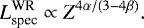
Recent calculations by Sander et al. (2019) reveal that there is also a transition in the wind regime for hydrogen-free WR stars. In Fig. 4, we show the behaviour of Ṁ (L) inferred from a series of hydrodynamically-consistent WN models with T* = 141 kK. For this, we calibrated their Ṁ(L∕M)-relation for Z⊙ with the L(M)-relation for He stars from Gräfener et al. (2011) in order to eliminate the explicit mass dependence. A power-law fit to the higher luminosity range confirms the empirical finding of a near-linear trend in this regime. However, the models also show that at lower luminosities (here ≈ 5.2 dex) there is a dramatic drop in the mass-loss rate that coincides with the eventual disappearance of the WR features in their spectrum. The luminosity cut-off in Fig. 4 is in agreement with observations of hot WR stars (see Fig. 3, right panel). However, given the various approximations made to derive this Ṁ (L)-relation, we do not expect it to exactly yield the observed threshold, which is set by cooler cWR stars with thin hydrogen mantels. To obtain a more accurate estimate, additional studies with hydrodynamical models accounting for the different temperatures and surface abundances would be required.
In the WR regime, by plugging Ṁ ∝ L in Eq. (1), one obtains Rt, WR ∝ L−1∕6. The small exponent implies that the dependence of secondary parameters on L (e.g., v∞) cannot be neglected in the WR regime, and hence one should not over-interpret the meaning of such a relation. However, once a critical luminosity has been reached, Ṁ drops abruptly primarily due to the transition to an optically-thin wind (Fig. 4), corresponding to an abrupt increase in Rt (Eq. (2)). This transition in Ṁ closely coincides with the disappearance of the WR features from the spectrum, implying that He stars below this luminosity threshold would not appear as WR stars. Hence, as observed, the WR phenomenon ceases below a relatively sharp luminosity threshold  . This luminosity threshold can be translated to a minimum He-star mass, which can in turn be translated into a minimum initial mass, Mi =
  .
.
We note that this derivation is valid for fixed temperature, terminal velocity, clumping factor, and composition. However, these parameters do generally depend on L. For example, lower-mass binary-stripped stars tend to be somewhat cooler and contain more hydrogen (e.g., Paczyński 1971; Götberg et al. 2018). Nevertheless, since we merely wish to motivate the existence of  in this section, this has little consequence on our final conclusion.
3.2 M increases with decreasing Z
The fact that  increases with decreasing Z should also not come as a surprise. The mass-loss rates of WN stars were reported to scale with Z roughly as ṀWR ∝ Z0.8 (Vink & de Koter 2005; Hainich et al. 2015; Shenar et al. 2019), with a shallower dependency reported for WC stars due to their self enrichment in metals (e.g., Tramper et al. 2016). Even though the ṀWR−Z relation may be more complex in truth, it is clear that, as Z decreases, larger He-core masses are needed to generate a WR spectrum. The threshold mass for the spectroscopic appearance of a WR star,
  , therefore increases with decreasing Z.
The HRD distributions of WR stars in the SMC, LMC, and MW enable us to determine  virtually without assumptions. This is especially the case for the SMC and LMC, in which the WR populations include all known apparently-single and binary WN stars. Moreover, WR stars close to the lower threshold of
  tend to exhibit weak emission lines blended with absorption, which strongly indicates that these WR stars are on the “verge” of appearing as Of stars. That is, we can be certain that we are sensitive to the lowest-luminosity WR stars.
From the populations shown in Fig. 3, we can draw threshold luminosities of approx. log = 5.6, 5.25, and 4.9 [L⊙] for the SMC, LMC, and MW, respectively. These values are estimated from the minimum WR luminosities in the respective galaxies, rounded to 0.05 dex. Clearly, the exact value would depend on the strict definition of WR stars, and is affected by uncertainties in log L (typically of the order of 0.1 dex), sample sizes, and completeness aspects. All in all, the exact values of
  are bound to beslightly subjective. However, our main argument, which will be outlined in Sect. 5, is not affected by such uncertainties.
We now convert these minimum threshold luminosities to minimum masses of WR stars. For this purpose, we use mass-luminosity relations published by Gräfener et al. (2011). We obtain  7.5, 11, and 17 M⊙. So, for example, a 10 M⊙ He star would appear as a WR star in the MW, but not in the SMC. These masses are consistent with dynamical masses measured in WR binaries in the MW (e.g., van der Hucht 2001), the LMC (e.g., Shenar et al. 2019), and the SMC (e.g., Shenar et al. 2016).
Translating these core masses back to progenitor masses is somewhat model-dependent, because it depends on the age of the He star and on the amount of mixing and rotation of the progenitor star. We discuss these uncertainties in more length in Appendix A. By estimating the most likely progenitor masses associated with the He-star masses derived above, we find  = 18, 24, and 37 M⊙ for the MW, LMC, and SMC, respectively. The inferred
  values for the different metallicities are compiled in Table 1.
One may notice that the values derived above for  appear to roughly follow
  ∝ Z−1, raising the question of whether this can be backed by theory. Let us again assume for simplicity that v∞, D, and R* do not depend on Z or L, and that Ṁ follows a relation in the form Ṁ ∝ Zα Lβ. Inserting all of this to Eq. (2), one finds Rt ∝ L(3−4β)∕6 Z−2α∕3. For constant Rt one obtains:
 (3)
(3)
Our values for  are calibrated using the lowest-luminosity WR stars, which, at least in the SMC and LMC, appear to have optically-thin winds (i.e., they are on the verge of being Of stars). Unlike typical WR stars, the mass-loss rates of such stars were shown to follow within considerable scatter the Ṁ−L relation derived by Vink (2017) for He stars with optically-thin winds (Shenar et al. 2019). Relying on this relation (α = 0.61 and β = 1.36), one obtains (at a rather astonishing accuracy)
  ∝ Z−1. However, considering the assumptions performed here (e.g., neglecting v∞ and T*) and the non-trivial dependence of Ṁ on Z (e.g., Sander et al. 2019), one must acknowledge that a theoretical prediction of
  (Z) needs to be confirmed with consistent models, which is beyond the scope of the current paper.
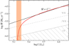 |
Fig. 4 Schematic behaviour of Ṁ as a functionof L for a hydrogen-free WN star with T* = 141 kK, based on the series of hydrodynamcially-consistent WN models at Z⊙ from Sander et al. (2019) and calibrations with the M(L)-relation from Gräfener et al. (2011). The upper dashed line indicates a linear trend in the WR regime, as confirmed from empirical measurements (see text). Lines of Rt = const (L ∝ Ṁ3∕4, see Eq. (2)) roughly indicate the regions in which a WR, /WR, and Of spectral appearance is obtained. The shaded orange region roughly marks the transition to a WR spectral appearance. We note that the curve and the position of the lines of Rt = const depend on the choice of T* and XH, and that the purpose of this figure is primarily illustrative. |
Values for  and
and  as a function of Z.
4 Estimating M: at what masses can single stars undergo self-stripping?
The parameter  has been extensively discussed in the literature. Up until a decade or so, a typical value for this parameter at Z = Z⊙ used to be cited as ≈25 M⊙ (e.g., Crowther 2007). Naive estimations of this parameter relied explicitly on calibration to the lowest-luminosity, apparently-single WR star. However, apparently-single WR stars may still have experienced binary interaction, and there are multiple scenarios to support this idea. To name a few: (1) the envelope of the WR progenitor could have been stripped during a second Roche lobe overflow phase onto a compact object (the original primary), and the once high-mass X-ray binary is now a long period WR + compact object binary in a quiescent state that escaped detection. (2) The progenitor of the WR star may have been stripped by a compact object or a lower mass object during common envelope evolution (Paczynski 1976; Schootemeijer & Langer 2018), where the lower-mass companion may have escaped detection. (3) After being stripped, the WR star was kicked away through three-body interactions in triple systems, becoming a single WR star with a history of binary interaction. (4) Some WR stars could be evolved merger products. The merging process may result in enhanced mass-loss due to super-Eddington winds and eruptions (e.g., Owocki et al. 2017) and enhanced rotation (e.g., de Mink et al. 2013). However, models calculated by Schneider et al. (2019) suggest the presence of strong magnetic fields in massive mergers, which may suppress both these phenomena. Whether a merger is more likely to become a WR star or not is, therefore, inconclusive.
Hence, calibrating evolution models to apparently-single WR stars can be very risky. Incidentally, we note that in all three galaxies, the lowest-luminosity WR stars are apparently single stars (Fig. 3). If we were to calibrate  according to them, we would naturally obtain
  =
=  , and the binary channel would be deemed irrelevant. However, there is no reason to suspect that the minimum mass necessary to appear as a WR star (
 ) is identical to the minimum mass necessary for a star to strip itself (
 ) in all three galaxies. Thus,
  cannot be derived from the empirical distribution of WR stars, and one needs to rely on the predictive power of evolution models.
The ability of a star to strip itself depends on two main factors: the mass-loss history of the star prior to the cWR phase (including eruptions), and the size of its convective core (mixing, rotation), including the interplay between the two. Needless to say, both these domains are hampered with uncertainties. Therefore, instead of trying to determine specific values for  , we examine predictions by various evolution codes. In Table 1, we summarize
  values obtained from the BPASS V2.0 (Eldridge et al. 2008; Eldridge & Stanway 2016), FRANEC (Limongi & Chieffi 2018), Geneva (Ekström et al. 2012; Georgy et al. 2012, 2015, Eggenberger et al. in prep.), and STARS (Dray & Tout 2003) stellar evolution codes, using various assumptions on rotation.
Values of  are not always stated by the authors. In these cases, we identify the lowest initial mass at which self-stripping occurs. We then interpolate between this value and the next-lowest initial mass in the corresponding grid to estimate
  . For example, as the Z = 0.002 BPASS single-star track for Mi = 50 M⊙ does not undergo self-stripping and Mi = 60 M⊙ track does, we estimate
  = 55 M⊙. We also note that the cWR phase is only considered to be reached if T* > 30 kk for the post main-sequence star. As can be seen from Fig. 3, no WR stars with log T*≲ 30 kK are known. This is different than the convention used by Georgy et al. (2012), for example, who defined the WR phase at T* ≥ 10 kK. Hence, the
  values given here may slightly deviate from values reported by the respective authors (e.g., compare Table 1 with Georgy et al. 2015).
The differences between the codes are abundant, and it is beyond the scope of our paper to discuss them in detail. Rather, Table 1 serves to give an impression of the uncertainties that dominate the parameter  , which become most extreme at low Z. For example, rotating FRANEC tracks at Z = 0.002 get to the cWR phase3 already at 35 M⊙, while rotating Geneva tracks barely reach the cWR phase even for the highest masses considered (120 M⊙). Instead of considering which of these predictions is closer to reality, we instead illustrate their consequence regarding the relative contributionof the binary channel.
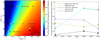 |
Fig. 5 Left: color map depicting the relative contribution of the binary channel (Eq. (4)) on the
|


5 The “window of opportunity” for the binary channel, [M,
M]
Binary stripping can primarily alter the number of WR stars in a given population for stars in the mass range  < Mi <
  : stars initially less massive than
  would not appear as WR stars after stripping. In contrast, stars more massive than
  would undergo self-stripping and rapidly enter the cWR phase as single stars, regardless of binary interactions. While the time-scales of the stripping could be slightly altered by the presence of a companion, the difference is negligible compared to the lifetime of the WR phenomenon, as is evident from the lack of red and yellow supergiants that correspond to Mi ≳ 30 M⊙ (e.g., Davies et al. 2018). The interval [
 (Z),
(Z),  (Z)] can therefore be considered as a “window of opportunity” for binary interactions to affect the WR population.
A few conclusions can be drawn immediately, just from the existence of this interval. For example, if for some reason  =
=  , that is to say, stars that appear as WR stars after stripping are stars that could strip themselves, then the additional contribution of the binary channel to the number of WR stars would vanish. If, in contrast,
  ≪
≪  , then the additional contribution would approach 100%, since virtually no WR stars could form as single stars except for perhaps the most massive stars.
We can quantify the additional contribution of the binary channel as follows. Using the terminology introduced by Shenar et al. (2019), let us use the designation b-WR star for a WR star that could only form through binary interactions, that is, a WR star with an initial mass in the interval [ ,
,  ]. Then the fraction of b-WR stars of the whole WR population would be:
 (4)
(4)
Here, Nb-WR∕NcWR is the fraction of WR stars that formed exclusively via the binary channel, fstrip is the fraction of stars successfully stripped by their companion, tWR is the lifetime of the cWR phase, and Mi, max is the upper mass limit of stars. The Salpeter initial mass function is assumed (Salpeter 1955). We adopt fstrip = 0.33 (Sana et al. 2012), and fix tWR to the He-burning lifetime (Hurley et al. 2002, Eq. (79)). We assume Mi, max = 300 M⊙ (e.g., Crowther et al. 2010), but note that the differences are indiscernible for Mi, max ≳ 200 M⊙.
In the left panel of Fig. 5, we show the values of Eq. (4) on the  –
– plane. We see that for
  ≫
≫  , the additional contribution of binaries to the WR population approaches unity, while for
  ≈
≈  , it vanishes. On the same plot, we mark the coordinates that correspond to the different predictions using the different codes, given in Table 1. In the right panel of Fig. 5, we plot the respective fractions as a function of Z. No coherenttrend arises from this plot, which is not surprising considering the vast differences in the predictions of the different codes. Moreover, none of the curves is monotonically increasing with decreasing Z. An exception to this is obtained when one assumes an upper mass limit of 150 M⊙, in which case Nb-WR∕NcWR in the Geneva models reaches 0.18, 0.77, and 0.80 in the MW, LMC, and SMC, respectively (i.e., very weakly monotonic).
The FRANEC rotating models are capable of stripping single stars at rather low masses, which is why the “window of opportunity” for binaries to take action is relatively small. At Z = Z⊙, rotating FRANEC tracks can actually strip at initial masses lower than  , which leaves no room for binaries to affect the number of WR stars in the MW. If true, this means that the Galaxy contains self-stripped stars that do not appear as WR stars, for which clear evidence still lacks. At Z = ZLMC,
  is slightly larger than
  , leaving some room for binaries to contribute at a 10% level. Going further to Z = ZSMC, the binary contributionremains modestly low, and even slightly decreases. Hence, assuming the FRANEC predictions are representative of realistic
  values, the additional contribution of binary interaction to the number of WR stars is virtually Z-independent, and is generally very low. The non-rotating FRANEC models are generally less successful in stripping stars, and result in a non-trivial dependence of the relative contribution of the binary channel on Z, with b-WR fractions ranging between 20–70%.
The Geneva rotating models behave similarly to the non-rotating FRANEC tracks, predicting at first an increase of the additional contribution of the binary channel from MW to LMC, and then a decrease. We note, however, that the initial rotation of 40% critical adopted by the Geneva models does not seem to agree with empirical measurements of rotational velocities of O-type stars (e.g., Ramírez-Agudelo et al. 2013, 2015). The BPASS tracks imply a somewhat intermediate behavior, with the relative contribution of the binary channel dropping between the MW and the LMC, and then increasing again at the SMC. Meanwhile, the STARS code implies a decrease of the additional contribution with decreasing Z–the opposite of the usual claim.
Despite these contradictory results, the conclusion is simple: the impact of binary interactions in forming WR stars depends on Z in a highly non-trivial manner. The additional contribution of the binary channel may increase or decrease with Z, depending on the metallicity regime. Hence, one should not expect a-priori that, at low Z, binaries are more important in forming WR stars, or that the WR binary fraction must increase.
6 Disclaimers
6.1 The apparent lack of a distinct mass interval
In our work, we motivate the existence of an initial-mass interval [ ,
,  ] in which WR stars can only form through binary interactions. The existence of this interval is the result of two seemingly straightforward facts, namely, the existence of
  (motivated in Sect. 3.1) and
  (a consensus in the literature). Yet the distributions of the apparently-single and binary WR stars in the SMC and LMC do not suggest the presence of such an interval. In fact, the SMC shows an opposite picture, where the low-luminosity WR stars appear to be single. From this, we conclude that at least one of the following should hold:
Binary evolution in disguise: the low-luminosity apparently-single WR stars may be products of binary evolution (e.g., Schootemeijer & Langer 2018), as we thoroughly discussed in Sect. 4. The apparent lack of a pure binary interval [
 ,
,  ] may be due to falsely assuming the apparently single stars are not the products of binary interaction.
Undetected binaries: due to observational biases, a population of WR binaries with bright mass-gainer companions may have avoided detection.
 ≈
≈  : it is possible that, in the SMC and LMC at least, stars that appear as WR stars after stripping are stars that undergo self-stripping. As this is not typically the prediction of evolution codes (cf. Table 1), this could imply (I) underestimated mass-loss rates (including eruptions); (II) underestimated mixing (due to rotation or otherwise).
Overestimated binary stripping: the initial conditions and detailed evolution of WR progenitors, which tend to be at the upper-mass range, are not well established. It is possible that the binary-stripping efficiency adopted here (fstrip = 0.33) is overestimated (e.g., because of decreased likelihood of interaction, or increased likelihood of merging, at the upper-mass range). While this alone does not help explain the existence of low-luminosity WR stars, it does help explain the apparent lack of low-luminosity WR binaries.
It is beyond the scope of the paper to investigate which of these scenarios is more likely to hold. More surveys of the WR stars will be needed to confirm or rule out the presence of hidden companions or additional WR binaries in the Magellanic Clouds. Moreover, a realistic treatment of rotation, binary interactions, and triple-body interactions should be implemented in evolution and models to examine whether these mechanisms can produce apparently-single low luminosity WR stars.
Regardless of which scenario holds: even if the interval [ ,
,  ] does not exist or is very small, it would still be consistent with binary interactions not becoming increasingly important in forming WR stars at low metallicities.
6.2 Uncertainties rooted in rotation
Rapid initial rotation tends to increase the size of the convective core and potentially boost the stellar mass-loss (e.g., Maeder & Meynet 2000). Therefore, enhanced rotation would generally tend to decrease the values of  and
and  in a non-trivial manner. Stars at lower Z are known to exhibit faster rotation on average (e.g., Ramírez-Agudelo et al. 2013; Ramachandran et al. 2019). It is therefore possible that distinct spin distributions at different metallicities indirectly impact the formation processes of WR stars as a function of Z.
It is difficult to predict the consequences this would have on the importance of binary interactions in forming WR stars. On the one hand, the effects of rotation become more prominent at low Z, which should generally increase the efficiency of the single-star channel in forming WR stars. On the other hand, it is possible that accretion of angular momentum during binary mass transfer contributes to the mixing of the mass gainer (e.g., Eldridge et al. 2017). If so, binary interactions may contribute to the formation of WR stars by forming rapidly rotating mass accretors (rather than through the stripping of the primaries alone). However, it is questionable whether mass-transfer can indeed efficiently mix the star after a chemical gradient has already been established.
All in all, the effects of rotation are extremely difficult to account for consistently given the multitude of mixing prescriptions and their interplay with binary interaction and mass-loss. This only stresses that the importance of binary interactions in forming WR stars is a non-trivial and strongly model-dependent variable.
6.3 Why binary interactions are important
The fact that the binary channel is not necessarily increasingly important for forming WR stars at low Z does not mean that binary interactions in general are not either. After all, it is clear that at low Z, mass-loss rates are smaller. How small they become is still debatable, since it is possible that Z-independent processes such as dust-driven winds (van Loon 2000) or eruptions (Smith 2014; Owocki et al. 2017) dominate the mass-loss at low Z. However, it is clear that, at low Z, binaries are expected to be an increasingly dominant agent for stripping. Hence, while we have shown that binary interactions may have a limited impact on the formation of WR stars (i.e., stars with a WR spectrum), it may still be the main channel with which He stars in general are formed.
Moreover, one should not confuse the incidence of binary interaction among WR stars with the additional contribution of the binary channel to the number of WR stars. Even if the additional contribution were low, it is still possible that the majority of WR stars interacted with a companion (e.g., Vanbeveren & Conti 1980). This may slightly affect the WR population: the presence of a companion may prevent the WR progenitor from becoming a red supergiant, and may therefore lead to longer WR lifetimes. We note, however, that the blatant lack of red supergiants with Mi ≳ 25 M⊙ (e.g., Humphreys & Davidson 1979; Davies et al. 2018) implies that WR progenitors spend a very short amount of time in this phase or skip it altogether.
Lastly, it is important to stress that this work does not “prove” that the additional contribution of the binary formation channel to the formation of WR stars is negligible. In principle, it only shows that there is no reason a-priori to believe that its influence on the WR population grows with decreasing Z.
7 Summary
In this work, we address the question of whether the WR binary fraction is truly expected to increase with decreasing Z, as is commonly claimed in the literature. We argued that stars with initial masses below a certain mass threshold  , which is a monotonically increasing function of Z, would not appear as WR stars spectroscopically. Using empirical HRD positions of WR stars in the SMC, LMC, and MW, we constrained minimum initial masses of
  = 18, 24, and 37 M⊙ for Z = 0.014, 0.006, and 0.002 (MW, LMC, SMC), respectively. Hence, for example, a star with an initial mass of Mi = 30 M⊙ would probably not appear as a WR star in the SMC after being stripped by a companion, but would do so in the Galaxy.
We continued by compiling the various predictions that exist for the well-known parameter  – the minimum initial mass above which stars reach the cWR phase through self-stripping. We relied on the FRANEC, BPASS, Geneva, and STARS evolution codes. The predictions of
  vary strongly between the codes, especially at low Z, and illustrate the large uncertainties involved in its calculation (see Table 1).
We argued that the binary channel can form additional WR stars primarily in the initial mass interval [ ,
,  ]. As both
  and
and  grow with decreasing Z, the additional contribution of the binary channel depends in a non-trivial manner on Z. Using the estimated values for
  and
and  for three distinct metallicities, and weighing against the initial mass function and the WR lifetime (Eq. (4)), we could produce predictions for the relative contribution of the binary channel.
Even though the results are heavily code-dependent and potentially affected by observational biases (see Sects. 6.1 and 6.2), one result emerges: within current uncertainties, no model can be claimed to conclusively predict a monotonically increasing behaviour (in fact, one of the models implies the opposite trend, see Fig. 5). In light of the uncertainties, we cannot rule out that binary interactions become increasingly important informing WR stars at low Z. Nonetheless,we have demonstrated in this paper that, contrary to common belief, this is not given a-priori. Thus, one should not prematurely expect that binary interactions dominate the formation of WR stars at low metallicity, or that the WR binary fraction should increase with decreasing Z.
Acknowledgements
We would like to thank our anonymous referee for their very critical and insightful comments - they have greatly contributed to our work. T.S. acknowledges support from the European Research Council (ERC) under the European Union’s DLV-772225-MULTIPLES Horizon 2020 research and innovation programme. A.A.C.S. is supported by STFC funding under grant number ST/R000565/1. T.S. would further like to thank insightful comments and inspiring conversations with A. F. J. Moffat, W.-R. Hamann, M. Limongi, R. Hainich, H. Todt, L. M. Oskinova, & N. Langer.
Appendix A Deriving M from
L
from
L
To estimate the initial mass  that corresponds to the luminosity of the He star
  , we use the binary module of Modules for Experiments in Stellar Astrophysics code (MESA, version 10 398, Paxton et al. 2011, 2013, 2015, 2018) to evolve stellar models with 33 different zero-age main sequence (ZAMS) primary masses between MZAMS = 10 M⊙ and MZAMS = 107 M⊙ with each model having a ZAMS secondary mass of half the primary mass. For the initial orbital period we use 12 values between Pi = 3 d and Pi = 10 000 d with logarithmic spacing. Two metallicity values are used, appropriate for the SMC and LMC. In total, 792 binary evolution tracks are generated.
Convective mixing employs a mixing-length parameter of αMLT = 1.5. Semiconvective mixing follows Langer et al. (1983) with an efficiency parameter of αsc = 1. We employ step overshooting above convective cores with αov = 0.335. All models are rotating with an initial rotation velocity of Vi = 100 km s−1, with the implementation of rotation in MESA described by Paxton et al. (2013), and the calibration of the mixing efficiency of Heger et al. (2000). Transport of angular momentum because of magnetic torques is according to Fuller et al. (2019).
Mass loss by stellar winds follows Vink et al. (2001) when T* > 10 kK and XH > 0.4. For T* < 10 kK the mass-loss prescription of de Jager et al. (1988) is employed. When Xs < 0.4 and the luminosity is below  we use the theoretical mass-loss rate of Vink (2017). For higher luminosities and when XH < 0.1 we follow either Hainich et al. (2014) or Tramper et al. (2016), depending on the surface helium mass fraction (see Yoon 2017 and Woosley 2019). Finally, for hot and luminous phases with 0.1 < XH < 0.4, we follow Nugis & Lamers (2000). Mass transfer by Roche lobe overflow follows the prescription of Kolb & Ritter (1990) with a mass transfer efficiency of zero, with the sole purpose of the mass transfer to strip the primary.
To get a mass-luminosity relation we find for each model the luminosity bin in which it spends the longest time, limiting to hot (log T* > 4.6[K]) post-MS (central hydrogen mass fraction below 0.01) phases, with each luminosity bin spanning Δlog L = 0.1 [L⊙]. We find that the duration spent in the derived luminosity bin is between 40 and 100% of the hot post-MS evolutionary phase we defined, and therefore yields a good representation of the mass-luminosity relation. The results are shown in Fig. A.1, where we also show the  values used in the paper.
 |
Fig. A.1 Luminosity bin in which each stellar model spent the longest time in its hot post-MS stage for SMC models (blue circles) and LMC models (orange squares). Our choice for
|


The method described above directly relates the luminosity of He stars to their ZAMS mass. This approach was chosen for simplicity. To conclude, we verify that this is consistent with the mass-luminosity relations of Gräfener et al. (2011). In Fig. A.2 we plot the mass-luminosity relation obtained from the stellar masses of our models when they are in their hot post-MS stage as defined above.
 |
Fig. A.2 Same as Fig. A.1, but with the x-axis showing the stellar mass at the beginning and at the end of the evolutionary phase in which the luminosity is in the longest-duration luminosity bin. |
Appendix B List of objects used in our analysis
In Table B.1, we list all WN stars used for our analysis. The results were adopted from Shenar et al. (2016, 2017, 2018, 2019), Hainich et al. (2014, 2015), Gvaramadze et al. (2014), Neugent et al. (2017), and Hamann et al. (2019).
SIMBAD designations of WR stars and binaries used in our analysis.
References
- Abbott, D. C., & Conti, P. S. 1987, ARA&A, 25, 113 [NASA ADS] [CrossRef] [Google Scholar]
- Bartzakos, P., Moffat, A. F. J., & Niemela, V. S. 2001, MNRAS, 324, 18 [NASA ADS] [CrossRef] [Google Scholar]
- Beals, C. S. 1940, JRASC, 34, 169 [NASA ADS] [Google Scholar]
- Bestenlehner, J. M., Gräfener, G., Vink, J. S., et al. 2014, A&A, 570, A38 [NASA ADS] [CrossRef] [EDP Sciences] [Google Scholar]
- Castor, J. I., Abbott, D. C., & Klein, R. I. 1975, ApJ, 195, 157 [NASA ADS] [CrossRef] [Google Scholar]
- Conti, P. S. 1976, Mem. Soc. R. Sci. Liège, 9, 193 [NASA ADS] [Google Scholar]
- Crowther, P. A. 2007, ARA&A, 45, 177 [NASA ADS] [CrossRef] [Google Scholar]
- Crowther, P. A., & Hadfield, L. J. 2006, A&A, 449, 711 [NASA ADS] [CrossRef] [EDP Sciences] [Google Scholar]
- Crowther, P. A., & Walborn, N. R. 2011, MNRAS, 416, 1311 [NASA ADS] [CrossRef] [MathSciNet] [Google Scholar]
- Crowther, P. A., Schnurr, O., Hirschi, R., et al. 2010, MNRAS, 408, 731 [NASA ADS] [CrossRef] [Google Scholar]
- Davies, B., Crowther, P. A., & Beasor, E. R. 2018, MNRAS, 478, 3138 [NASA ADS] [CrossRef] [Google Scholar]
- de Jager, C., Nieuwenhuijzen, H., & van der Hucht, K. A. 1988, A&AS, 72, 259 [NASA ADS] [Google Scholar]
- de Koter, A., Heap, S. R., & Hubeny, I. 1997, ApJ, 477, 792 [Google Scholar]
- de Mink, S. E., Langer, N., Izzard, R. G., Sana, H., & de Koter, A. 2013, ApJ, 764, 166 [NASA ADS] [CrossRef] [Google Scholar]
- Dray, L. M., & Tout, C. A. 2003, MNRAS, 341, 299 [NASA ADS] [CrossRef] [Google Scholar]
- Dunstall, P. R., Dufton, P. L., Sana, H., et al. 2015, A&A, 580, A93 [NASA ADS] [CrossRef] [EDP Sciences] [Google Scholar]
- Ekström, S., Georgy, C., Eggenberger, P., et al. 2012, A&A, 537, A146 [NASA ADS] [CrossRef] [EDP Sciences] [Google Scholar]
- Eldridge, J. J., & Stanway, E. R. 2016, MNRAS, 462, 3302 [NASA ADS] [CrossRef] [Google Scholar]
- Eldridge, J. J., Izzard, R. G., & Tout, C. A. 2008, MNRAS, 384, 1109 [NASA ADS] [CrossRef] [Google Scholar]
- Eldridge, J. J., Stanway, E. R., Xiao, L., et al. 2017, PASA, 34, e058 [NASA ADS] [CrossRef] [Google Scholar]
- Foellmi, C., Moffat, A. F. J., & Guerrero, M. A. 2003a, MNRAS, 338, 360 [NASA ADS] [CrossRef] [Google Scholar]
- Foellmi, C., Moffat, A. F. J., & Guerrero, M. A. 2003b, MNRAS, 338, 1025 [NASA ADS] [CrossRef] [Google Scholar]
- Fuller, J., Piro, A. L., & Jermyn, A. S. 2019, MNRAS, 485, 3661 [NASA ADS] [Google Scholar]
- Fullerton, A. W., Massa, D. L., & Prinja, R. K. 2006, ApJ, 637, 1025 [NASA ADS] [CrossRef] [Google Scholar]
- Georgy, C., Ekström, S., Meynet, G., et al. 2012, A&A, 542, A29 [NASA ADS] [CrossRef] [EDP Sciences] [Google Scholar]
- Georgy, C., Ekström, S., Hirschi, R., et al. 2015, in Wolf-Rayet Stars: Proc. Int. Workshop held in Potsdam, Germany, eds. W.-R. Hamann, A. Sander, & H. Todt, Universitätsverlag Potsdam, 229 [Google Scholar]
- Gilkis, A., Vink, J. S., Eldridge, J. J., & Tout, C. A. 2019, MNRAS, 486, 4451 [NASA ADS] [CrossRef] [Google Scholar]
- Götberg, Y., de Mink, S. E., Groh, J. H., et al. 2018, A&A, 615, A78 [NASA ADS] [CrossRef] [EDP Sciences] [Google Scholar]
- Gräfener, G., & Hamann, W.-R. 2005, A&A, 432, 633 [NASA ADS] [CrossRef] [EDP Sciences] [Google Scholar]
- Gräfener, G., Koesterke, L., & Hamann, W.-R. 2002, A&A, 387, 244 [NASA ADS] [CrossRef] [EDP Sciences] [Google Scholar]
- Gräfener, G., Vink, J. S., de Koter, A., & Langer, N. 2011, A&A, 535, A56 [NASA ADS] [CrossRef] [EDP Sciences] [Google Scholar]
- Groh, J. H., Oliveira, A. S., & Steiner, J. E. 2008, A&A, 485, 245 [NASA ADS] [CrossRef] [EDP Sciences] [Google Scholar]
- Groh, J. H., Ekström, S., Georgy, C., et al. 2019, A&A, 627, A24 [NASA ADS] [CrossRef] [EDP Sciences] [Google Scholar]
- Gvaramadze, V. V., Chené, A. N., Kniazev, A. Y., et al. 2014, MNRAS, 442, 929 [NASA ADS] [CrossRef] [Google Scholar]
- Hainich, R., Rühling, U., Todt, H., et al. 2014, A&A, 565, A27 [NASA ADS] [CrossRef] [EDP Sciences] [Google Scholar]
- Hainich, R., Pasemann, D., Todt, H., et al. 2015, A&A, 581, A21 [Google Scholar]
- Hamann, W. R., & Gräfener, G. 2003, A&A, 410, 993 [NASA ADS] [CrossRef] [EDP Sciences] [Google Scholar]
- Hamann, W. R., Koesterke, L., & Wessolowski, U. 1993, A&A, 274, 397 [NASA ADS] [Google Scholar]
- Hamann, W. R., Gräfener, G., Liermann, A., et al. 2019, A&A, 625, A57 [NASA ADS] [CrossRef] [EDP Sciences] [Google Scholar]
- Heger, A., Langer, N., & Woosley, S. E. 2000, ApJ, 528, 368 [NASA ADS] [CrossRef] [Google Scholar]
- Humphreys, R. M., & Davidson, K. 1979, ApJ, 232, 409 [NASA ADS] [CrossRef] [Google Scholar]
- Hunter, I., Dufton, P. L., Smartt, S. J., et al. 2007, A&A, 466, 277 [NASA ADS] [CrossRef] [EDP Sciences] [Google Scholar]
- Hurley, J. R., Tout, C. A., & Pols, O. R. 2002, MNRAS, 329, 897 [NASA ADS] [CrossRef] [Google Scholar]
- Kolb, U., & Ritter, H. 1990, A&A, 236, 385 [NASA ADS] [Google Scholar]
- Langer, N. 2012, ARA&A, 50, 107 [NASA ADS] [CrossRef] [Google Scholar]
- Langer, N., Fricke, K. J., & Sugimoto, D. 1983, A&A, 126, 207 [NASA ADS] [Google Scholar]
- Leuenhagen, U., & Hamann, W. R. 1998, A&A, 330, 265 [NASA ADS] [Google Scholar]
- Limongi, M., & Chieffi, A. 2018, ApJS, 237, 13 [NASA ADS] [CrossRef] [Google Scholar]
- Lucy, L. B., & Abbott, D. C. 1993, ApJ, 405, 738 [NASA ADS] [CrossRef] [Google Scholar]
- Maeder, A., & Meynet, G. 1994, A&A, 287, 803 [Google Scholar]
- Maeder, A., & Meynet, G. 2000, A&A, 361, 159 [NASA ADS] [Google Scholar]
- Massey, P., Olsen, K. A. G., & Parker, J. W. 2003, PASP, 115, 1265 [NASA ADS] [CrossRef] [Google Scholar]
- Massey, P., Neugent, K. F., Morrell, N., & Hillier, D. J. 2014, ApJ, 788, 83 [NASA ADS] [CrossRef] [Google Scholar]
- Moe, M., Kratter, K. M., & Badenes, C. 2019, ApJ, 875, 61 [NASA ADS] [CrossRef] [Google Scholar]
- Neugent, K. F., & Massey, P. 2014, ApJ, 789, 10 [NASA ADS] [CrossRef] [EDP Sciences] [Google Scholar]
- Neugent, K., & Massey, P. 2019, Galaxies, 7, 74 [NASA ADS] [CrossRef] [Google Scholar]
- Neugent, K. F., Massey, P., Hillier, D. J., & Morrell, N. 2017, ApJ, 841, 20 [NASA ADS] [CrossRef] [Google Scholar]
- Neugent, K. F., Massey, P., & Morrell, N. 2018, ApJ, 863, 181 [NASA ADS] [CrossRef] [Google Scholar]
- Nugis, T., & Lamers, H. J. G. L. M. 2000, A&A, 360, 227 [NASA ADS] [Google Scholar]
- Oskinova, L. M., Hamann, W.-R., & Feldmeier, A. 2007, A&A, 476, 1331 [NASA ADS] [CrossRef] [EDP Sciences] [Google Scholar]
- Owocki, S. P., Townsend, R. H. D., & Quataert, E. 2017, MNRAS, 472, 3749 [Google Scholar]
- Paczyński, B. 1967, Acta Astron., 17, 355 [NASA ADS] [Google Scholar]
- Paczyński, B. 1971, Acta Astron., 21, 1 [NASA ADS] [Google Scholar]
- Paczynski, B. 1976, IAU Symp., 73, 75 [NASA ADS] [EDP Sciences] [Google Scholar]
- Paxton, B., Bildsten, L., Dotter, A., et al. 2011, ApJS, 192, 3 [Google Scholar]
- Paxton, B., Cantiello, M., Arras, P., et al. 2013, ApJS, 208, 4 [NASA ADS] [CrossRef] [Google Scholar]
- Paxton, B., Marchant, P., Schwab, J., et al. 2015, ApJS, 220, 15 [Google Scholar]
- Paxton, B., Schwab, J., Bauer, E. B., et al. 2018, ApJS, 234, 34 [NASA ADS] [CrossRef] [EDP Sciences] [Google Scholar]
- Prentice, S. J., Ashall, C., James, P. A., et al. 2019, MNRAS, 485, 1559 [NASA ADS] [CrossRef] [Google Scholar]
- Puls, J., Markova, N., Scuderi, S., et al. 2006, A&A, 454, 625 [NASA ADS] [CrossRef] [EDP Sciences] [Google Scholar]
- Ramachandran, V., Hamann, W. R., Oskinova, L. M., et al. 2019, A&A, 625, A104 [NASA ADS] [CrossRef] [EDP Sciences] [Google Scholar]
- Ramírez-Agudelo, O. H., Simón-Díaz, S., Sana, H., et al. 2013, A&A, 560, A29 [NASA ADS] [CrossRef] [EDP Sciences] [Google Scholar]
- Ramírez-Agudelo, O. H., Sana, H., de Mink, S. E., et al. 2015, A&A, 580, A92 [NASA ADS] [CrossRef] [EDP Sciences] [Google Scholar]
- Salpeter, E. E. 1955, ApJ, 121, 161 [Google Scholar]
- Sana, H., de Mink, S. E., de Koter, A., et al. 2012, Science, 337, 444 [Google Scholar]
- Sana, H., de Koter, A., de Mink, S. E., et al. 2013, A&A, 550, A107 [NASA ADS] [CrossRef] [EDP Sciences] [Google Scholar]
- Sander, A., Shenar, T., Hainich, R., et al. 2015, A&A, 577, A13 [NASA ADS] [CrossRef] [EDP Sciences] [Google Scholar]
- Sander, A. A. C., Hamann, W.-R., Todt, H., Hainich, R., & Shenar, T. 2017, A&A, 603, A86 [NASA ADS] [CrossRef] [EDP Sciences] [Google Scholar]
- Sander, A. A. C., Vink, J. S., & Hamann, W. R. 2019, MNRAS, 2641 [Google Scholar]
- Schmutz, W., Hamann, W.-R., & Wessolowski, U. 1989, A&A, 210, 236 [NASA ADS] [Google Scholar]
- Schneider, F. R. N., Ohlmann, S. T., Podsiadlowski, P., et al. 2019, Nature, 574, 211 [NASA ADS] [CrossRef] [Google Scholar]
- Schnurr, O., Moffat, A. F. J., St-Louis, N., Morrell, N. I., & Guerrero, M. A. 2008, MNRAS, 389, 806 [NASA ADS] [CrossRef] [Google Scholar]
- Schootemeijer,A., & Langer, N. 2018, A&A, 611, A75 [NASA ADS] [CrossRef] [EDP Sciences] [Google Scholar]
- Shenar, T., Hainich, R., Todt, H., et al. 2016, A&A, 591, A22 [NASA ADS] [CrossRef] [EDP Sciences] [Google Scholar]
- Shenar, T., Richardson, N. D., Sablowski, D. P., et al. 2017, A&A, 598, A85 [NASA ADS] [CrossRef] [EDP Sciences] [Google Scholar]
- Shenar, T., Hainich, R., Todt, H., et al. 2018, A&A, 616, A103 [NASA ADS] [CrossRef] [EDP Sciences] [Google Scholar]
- Shenar, T., Sablowski, D. P., Hainich, R., et al. 2019, A&A, 627, A151 [NASA ADS] [CrossRef] [EDP Sciences] [Google Scholar]
- Smartt, S. J. 2009, ARA&A, 47, 63 [NASA ADS] [CrossRef] [Google Scholar]
- Smith, N. 2014, ARA&A, 52, 487 [NASA ADS] [CrossRef] [MathSciNet] [Google Scholar]
- Sota, A., Maíz Apellániz, J., Morrell, N. I., et al. 2014, ApJS, 211, 10 [NASA ADS] [CrossRef] [Google Scholar]
- Steiner, J. E., & Oliveira, A. S. 2005, A&A, 444, 895 [NASA ADS] [CrossRef] [EDP Sciences] [Google Scholar]
- Sundqvist, J. O., & Puls, J. 2018, A&A, 619, A59 [NASA ADS] [CrossRef] [EDP Sciences] [Google Scholar]
- Sundqvist, J. O., Björklund, R., Puls, J., & Najarro, F. 2019, A&A, 632, A126 [NASA ADS] [CrossRef] [EDP Sciences] [Google Scholar]
- Tramper, F., Sana, H., & de Koter, A. 2016, ApJ, 833, 133 [NASA ADS] [CrossRef] [Google Scholar]
- Vanbeveren, D., & Conti, P. S. 1980, A&A, 88, 230 [NASA ADS] [Google Scholar]
- van der Hucht, K. A. 2001, New Astron. Rev., 45, 135 [NASA ADS] [CrossRef] [Google Scholar]
- van Loon, J. T. 2000, A&A, 354, 125 [NASA ADS] [Google Scholar]
- Vink, J. S. 2017, A&A, 607, L8 [NASA ADS] [CrossRef] [EDP Sciences] [Google Scholar]
- Vink, J. S., & de Koter, A. 2005, A&A, 442, 587 [NASA ADS] [CrossRef] [EDP Sciences] [Google Scholar]
- Vink, J. S., & Gräfener, G. 2012, ApJ, 751, L34 [NASA ADS] [CrossRef] [Google Scholar]
- Vink, J. S., de Koter, A., & Lamers, H. J. G. L. M. 2001, A&A, 369, 574 [NASA ADS] [CrossRef] [EDP Sciences] [Google Scholar]
- Vink, J. S., Muijres, L. E., Anthonisse, B., et al. 2011, A&A, 531, A132 [NASA ADS] [CrossRef] [EDP Sciences] [Google Scholar]
- Woosley, S. E. 2019, ApJ, 878, 49 [NASA ADS] [CrossRef] [Google Scholar]
- Yoon, S.-C. 2017, MNRAS, 470, 3970 [NASA ADS] [CrossRef] [Google Scholar]
Throughout this paper, only massive stars and their WR counterparts are considered. The low-mass central WR stars of planetary nebula – so called [WR] stars – obey a different mass-luminosity relation (e.g., Leuenhagen & Hamann 1998), and are not regarded here.
According to Limongi & Chieffi (2018), at metallicities of roughly Z = 0.002 and lower, dust-driven winds during the red supergiant phase dominate the mass removal, making  independent of Z.
All Tables
All Figures
|
Fig. 1 Illustration of the minimum initial mass required to appear as a WR star after stripping ( |
| In the text | |
|
Fig. 2 Synthetic PoWR spectra calculated for fixed parameters (T* = 50 kK, log L = 5.3 [L⊙], M = 13 M⊙, v∞ = 1000 km s−1, D = 10, surface hydrogen mass fraction XH = 0.4, LMC-like composition) but different Rt (see legend). The figure illustrates that stars with Rt values above a certain threshold would not appear as WR stars. |
| In the text | |
|
Fig. 3 Observed populations of WR stars in the SMC (left panel), LMC (middle panel), and MW (right panel). The SMC and LMC populations include both apparently single WN stars (Hainich et al. 2014, 2015, gray circles), WN binaries (Gvaramadze et al. 2014; Shenar et al. 2016, 2017, 2018, 2019, gray circles surrounded by red circles), and the so-calledLMC WN3/O3 stars (Neugent et al. 2017, gray triangles). The MW sample includes only apparently-single WN stars (Hamann et al. 2019). Marked are the lowest luminosities measured for WR stars in each respective galaxy, rounded to 0.05 dex, where a clear metallicity trend is apparent. |
| In the text | |
|
Fig. 4 Schematic behaviour of Ṁ as a functionof L for a hydrogen-free WN star with T* = 141 kK, based on the series of hydrodynamcially-consistent WN models at Z⊙ from Sander et al. (2019) and calibrations with the M(L)-relation from Gräfener et al. (2011). The upper dashed line indicates a linear trend in the WR regime, as confirmed from empirical measurements (see text). Lines of Rt = const (L ∝ Ṁ3∕4, see Eq. (2)) roughly indicate the regions in which a WR, /WR, and Of spectral appearance is obtained. The shaded orange region roughly marks the transition to a WR spectral appearance. We note that the curve and the position of the lines of Rt = const depend on the choice of T* and XH, and that the purpose of this figure is primarily illustrative. |
| In the text | |
|
Fig. 5 Left: color map depicting the relative contribution of the binary channel (Eq. (4)) on the
|
| In the text | |
|
Fig. A.1 Luminosity bin in which each stellar model spent the longest time in its hot post-MS stage for SMC models (blue circles) and LMC models (orange squares). Our choice for
|
| In the text | |
|
Fig. A.2 Same as Fig. A.1, but with the x-axis showing the stellar mass at the beginning and at the end of the evolutionary phase in which the luminosity is in the longest-duration luminosity bin. |
| In the text | |
Current usage metrics show cumulative count of Article Views (full-text article views including HTML views, PDF and ePub downloads, according to the available data) and Abstracts Views on Vision4Press platform.
Data correspond to usage on the plateform after 2015. The current usage metrics is available 48-96 hours after online publication and is updated daily on week days.
Initial download of the metrics may take a while.