| Issue |
A&A
Volume 634, February 2020
|
|
|---|---|---|
| Article Number | A20 | |
| Number of page(s) | 7 | |
| Section | The Sun | |
| DOI | https://doi.org/10.1051/0004-6361/201936861 | |
| Published online | 30 January 2020 | |
Toward a realistic macroscopic parametrization of space plasmas with regularized κ-distributions
1
Centre for Mathematical Plasma Astrophysics, Celestijnenlaan 200B, 3001 Leuven, Belgium
2
Institute for Theoretical Physics IV, Ruhr-University Bochum, 44780 Bochum, Germany
e-mail: mlazar@tp4.rub.de
3
Research Dept. Plasmas with Complex Interactions, Ruhr-University Bochum, 44780 Bochum, Germany
4
Space Physics Department and STCE, Royal Belgian Institute for Space Aeronomy, 1180 Brussels, Belgium
5
ELI-C (Earth Life Institute), Université Catholique de Louvain (UCLouvain), 1348 Louvain-La-Neuve, Belgium
Received:
7
October
2019
Accepted:
20
December
2019
So-called κ-distributions are widely invoked in the analysis of nonequilibrium plasmas from space, although a general macroscopic parametrization as known for Maxwellian plasmas near thermal equilibrium is prevented by the diverging moments of order l ≥ 2κ − 1. To overcome this critical limitation, recently novel regularized κ-distributions (RK) have been introduced, including various anisotropic models with well-defined moments for any value of κ > 0. In this paper, we present an evaluation of the pressure and heat flux of electron populations, as provided by moments of isotropic and anisotropic RKs for conditions typically encountered in the solar wind. We obtained finite values even for low values of κ < 3/2, for which the pressure and heat flux moments of standard κ-distributions are not defined. These results were also contrasted with the macroscopic parameters obtained for Maxwellian populations, which show a significant underestimation especially if an important suprathermal population is present (e.g., for κ < 2), but ignored. Despite the collisionless nature of solar wind plasma, a realistic characterization as a fluid becomes thus possible, retaining all nonthermal features of plasma particles.
Key words: solar wind / plasmas / methods: statistical
© ESO 2020
1. Introduction
Collision-poor plasmas from astrophysical and experimental setups cannot easily reach thermal equilibrium. Plasma particles exhibit non-Maxwellian velocity distributions that are well represented by the κ-power laws (Vasyliunas 1968; Collier et al. 1996; Maksimovic et al. 2005; Štverák et al. 2008), including isotropic and anisotropic κ-distribution functions which greatly facilitate descriptions of plasma effects at small scales; see Pierrard & Lazar (2010) for a review. These departures from thermal equilibrium are expected as a consequence of long-range (collective) interactions of plasma particles mediated by electromagnetic field fluctuations (Treumann et al. 2004; Leubner & Vörös 2005). Scenarios based on the existence of κ-distributions are widely invoked, especially in the expansion of solar atmosphere, to explain coronal plasma heating (Scudder 1992), differential acceleration of the solar wind (Maksimovic et al. 1997), and its interaction with planetary environments (Meyer-Vernet 2001). These scenarios may also offer indirect insights from the physics of nonthermal emissions, as observed from flaring sources in the solar corona (Dudík et al. 2017) or from more distant astrophysical objects (Nicholls et al. 2012).
Similar to a standard Maxwellian for plasmas at (or near) thermal equilibrium, the main moments of the velocity distribution are expected to provide a macroscopic characterization of nonequilibrium plasmas, but moments of a κ-distribution are however not well defined for any value of κ (Scherer et al. 2017, 2019a). Thus, the moment of order l can be defined only for κ > (l + 1)/2, and the pressure (or kinetic temperature) parameter is notorious, being directly derived from the moment of order l = 2, which is convergent only for κ > 3/2. If the temperature is taken as a fitting parameter, the observations not satisfying this condition are simply discarded and lost from the analysis (Štverák et al. 2008), leading to questionable or even unrealistic interpretations. In order to overcome these limitations, standard κ-distributions have recently been adjusted by introducing the regularized κ-distribution (RK) with well-defined moments for any value of κ > 0 (Scherer et al. 2017). General expressions of the principal moments (l ≤ 3) were also provided for various anisotropic RKs, able to describe temperature anisotropies or drifting populations, see Scherer et al. (2019a).
These recent results are applied in the present paper to evaluate the main properties of electron populations, for example, pressure P (or temperature T) given by the second-order moment and the heat flux derived from the third-order moment. We chose conditions typically observed in the solar wind, where plasma particles are predominantly nonrelativistic (kBT ≪ mc2) and the main heat-flux is carried by the beaming populations, i.e., by the electron strahl. The solar wind is not highly magnetized, for instance, at 1 AU the electron plasma frequency is much higher than cyclotron frequency, but the interplanetary magnetic field ensures a gyrotropy of the velocity distributions, i.e., the distributions are almost isotropic in the plane perpendicular (subscript ⊥) to the magnetic field (Maksimovic et al. 2005; Štverák et al. 2008). Thus, deviations from isotropy in general take the form of electron beams (or strahls) propagating parallel (subscript ∥) to the magnetic field and anisotropic pressure P (or temperature T) of electron populations with different components P⊥ ≠ P∥ (or T⊥ ≠ T∥).
In Sect. 2 we consider non-drifting electrons associated with central populations in the observed distributions (Štverák et al. 2008), i.e., the core and halo electrons, which are together well reproduced by a κ-distribution function (Lazar et al. 2017) without a major drift with respect to the massive ions. In the solar wind (ions) referential the net heat flux of these electron populations is zero, and we may restrict the analysis to the pressure (or temperature) components. Additional drifting or beaming electrons responsible for the electron heat flux are enhanced in fast winds or during more energetic events like coronal mass ejections (CMEs). These electron beams or strahls are nonthermal and are well described by the same κ-distribution functions with field-aligned drifts (Nieves-Chinchilla & Viñas 2008; Štverák et al. 2009; Viñas et al. 2010; Lazar et al. 2017). In Sect. 3 we evaluate the pressure components and the (parallel) heat flux transported by the electron beams with isotropic or anisotropic pressures. Macroscopic properties predicted for RKs are compared with the corresponding moments of standard κ-distributions. These properties are also contrasted with Maxwellian limits reproducing the core of the observed distributions, which are often invoked to motivate a fluid description and ignore suprathermal populations. In the last section we summarize the present results and discuss their importance from a perspective of a realistic macroscopic characterization of space plasmas as fluids.
2. Non-drifting distributions
We assume a plasma of electrons (subscript e) and protons (subscript p) specific to the solar wind conditions at 1 AU. The following basic set of plasma parameters characterizes the low-energy core or Maxwelian populations: number densities ne = np = n0 = 10 cm−3; temperatures Te ≃ Tp = 105 K, implying a mean energy per electron kBTe ≃ 8.6 eV and for thermal velocity of electrons θ = (2kBTe/me)1/2 ≃ 0.005c, where c is the speed of light in vacuum; and magnetic field B0 = 10−4G = 10 nT, implying for the ratio of plasma and cyclotron frequencies ωpe/ωce ≃ 100. These values are used in our evaluations for each type of κ-distribution function, standard or regularized, intended to account for suprathermal electrons and their contribution to the macroscopic properties of solar wind plasma. Heavier ions may also be present in the solar wind but usually with a very low number density ni/ntotal < 4%, and these are therefore ignored in the present analysis.
2.1. Isotropic temperatures
For isotropic temperatures T∥ = T⊥ = T the observed velocity distributions are described by a standard κ-distribution function, denoted with subscript K (Appendix A summarizes the abbreviations used for the distribution functions), i.e.,
![$$ \begin{aligned} f_{K}(v) = { n_0\Gamma [\kappa ] \over (\pi \theta ^2 \kappa )^{3/2} \Gamma [\kappa -1/2]} \left(1 + \frac{v^{2}}{\kappa \theta ^2}\right)^{-\kappa -1}, \end{aligned} $$](/articles/aa/full_html/2020/02/aa36861-19/aa36861-19-eq1.gif)
where θ is given by the second order moment kBT = (2/3)(m < v2 > /2) = (m/3)∫d3v v2fK = (mθ2/2) κ/(κ − 3/2). The same θ may be associated with the Maxwellian (subscript M) limit (Lazar et al. 2015, 2016)
describing the core (low-energy) population in the observed distribution (assuming ncore ≃ n0). Thermal velocity of the core electrons is directly related to their temperature by θ = (2kBTM/m)1/2.
The regularized κ-distribution (subscript RK; Scherer et al. 2017)
![$$ \begin{aligned} f_{\rm RK}(v) = {n_0 \;_{[]}\mathcal{U} _{[0]} \over (\pi \theta ^2 \kappa )^{3/2}} \left(1+ {v^2 \over \kappa \theta ^2}\right)^{-\kappa -1} \exp \left(-\alpha ^{2} v^{2} \over \theta ^2 \right) \end{aligned} $$](/articles/aa/full_html/2020/02/aa36861-19/aa36861-19-eq3.gif)
combines standard κ-distribution with an exponential cutoff controlled by the positive cutoff parameter α < 1, which must be small enough such that the RK retains the relevance of extended suprathermal tails in the observed distributions. In the normalization constant
![$$ \begin{aligned} _{[n]}\mathcal{U} _{[]} = 1/ _{[]}\mathcal{U} _{[n]} = U\left({3+n \over 2}, {3+n \over 2} - \kappa , \alpha ^2 \kappa \right), \end{aligned} $$](/articles/aa/full_html/2020/02/aa36861-19/aa36861-19-eq4.gif)
where U(a, b, z) is the Kummer U (or Tricomi) function (Scherer et al. 2019a). For α = 0 the RK reduces to a standard κ-distribution, but a finite value α > θ/c is required for the cutoff parameter in order to restrain for speeds lower than the speed of light c in vacuum and to minimize the unrealistic effects of superluminal particles with v > c (Scherer et al. 2019b). For the solar wind plasma conditions assumed in this work, we find α = 0.012 large enough to admit only negligible effects of superluminal particles (see condition RR < 1% for the relative pressure contribution of superluminal particles in Scherer et al. (2019b)) satisfied in this case for any value of κ > 0. With this value for α we use the results in Scherer et al. (2019a) to evaluate the relative pressures Pi/PM, and obtain
for a standard κ-distribution, and
![$$ \begin{aligned} P_{RK} / P_M = \kappa \; _{[2]}\mathcal{U} _{[0]}, \end{aligned} $$](/articles/aa/full_html/2020/02/aa36861-19/aa36861-19-eq6.gif)
for RK, where PM = (1/2)n0meθ2 ≃ 1.2 10−11 N m−2 is the pressure given by Maxwellian limit in Eq. (2) (with the parameters from above)1. Normalized pressures are plotted in Fig. 1 as a function of κ. Variations with κ of the normalized temperatures TRK/TM and TK/TM have the same profiles (not shown here) as PRK/PM and PK/PM, respectively. These profiles tend to coincide for large values of κ > 10, stating that this happens only in the absence of suprathermal populations. Most probably, very strong suprathermal tails corresponding to very low values of κ < 1 and to PRK (or TRK) values several orders of magnitude higher than PM (or TM) are not encountered in the solar wind. However, distributions corresponding to moderately low values of κ < 10 are more expected; these distibutions include those slightly below the limit imposed by a standard κ-distribution (subscript K), i.e., 1 ≤ κ ≤ 3/2, which are usually discarded if fitted with such a power-law model (Štverák et al. 2008). The bottom panel of Fig. 1 shows only this interval of κ values, where the pressure (or the temperature) is highly dependent on the model function for the observed velocity distribution. For instance, we can evaluate the relative pressure for κ = 1, and find PRK/PM = 62.4, implying for the absolute pressure PRK ≃ 0.7 10−9 N m−2 > PM, that means a boost of at least one order of magnitude under the effects of suprathermals. For κ > 3/2 these parameters can be evaluated for a standard K, but leading to overestimations. For instance, for κ = 1.6 we find PK/PM = 16, roughly two times higher than PRK/PM = 7.65, which leads to a realistic value PRK ≃ 0.9 10−10 N m−2.
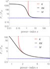 |
Fig. 1. Normalized pressure Pi/PM for a standard (isotropic) κ-distribution (i = K, red dashed) and for the regularized κ-distribution (i = RK, black solid) in bottom panel with a zoom-in only for a restraint range of conditions relevant for the solar wind. |
2.2. Anisotropic temperatures
For anisotropic temperatures T∥ ≠ T⊥, where ∥ and ⊥ denote directions relative to the uniform magnetic field lines, the observed velocity distributions can be described by a bi-κ-distribution (subscript BK; Maksimovic et al. 2005; Štverák et al. 2008)
![$$ \begin{aligned} f_{\rm BK}(v_\parallel , v_\perp ) = { n_0 \Gamma [\kappa ] \over (\pi \kappa )^{3/2} \theta _\parallel \theta _\perp ^2 \Gamma [\kappa -1/2]} \left(1 + \frac{v_\parallel ^{2}}{\kappa \theta _\parallel ^2} + \frac{v_\perp ^{2}}{\kappa \theta _\perp ^2}\right)^{-\kappa -1}, \end{aligned} $$](/articles/aa/full_html/2020/02/aa36861-19/aa36861-19-eq7.gif)
where θ∥, ⊥ are given by the second-order moment  . The same θ∥, ⊥ = (2kBTM, ∥, ⊥/m)1/2 describe the anisotropic (low-energy) core within a bi-Maxwellian (subscript BM)
The regularized bi-κ-distribution (subscript RBK, see also Appendix A for a summary of these abbreviations)
![$$ \begin{aligned} f_{\rm RBK}(v_{\parallel }, v_\perp )&= {n_0 \;_{[0]}\mathcal{U} _{[]} \over (\pi \kappa )^{3/2}\theta _\parallel \theta _\perp ^2} \left(1 + \frac{v_\parallel ^{2}}{\kappa \theta _\parallel ^2} + \frac{v_\perp ^{2}}{\kappa \theta _\perp ^2}\right)^{-\kappa -1} \nonumber \\&\quad \times \exp \left(- \frac{\alpha ^2 v_\parallel ^{2}}{\theta _\parallel ^2} - \frac{\alpha ^2 v_\perp ^{2}}{\theta _\perp ^2}\right) \end{aligned} $$](/articles/aa/full_html/2020/02/aa36861-19/aa36861-19-eq10.gif)
combines a BK function with an exponential cutoff factor controlled by a small α < 1 (Scherer et al. 2019a). This cutoff parameter can be directly related to the maximum energy channel of the instrument measuring the particle distributions independently, which is the same for all pitch angles. Different cutoffs corresponding to parallel and perpendicular directions α∥ ≠ α⊥ may introduce additional anisotropies (Scherer et al. 2019a), which are not of interest in the present study. For α = 0 the RBK reduces to a standard BK, but again a finite value α > θ/c is required for the cutoff parameter to restrain to realistic speeds v < c (Scherer et al. 2019b), such that for the solar wind conditions at 1 AU we find α = 0.012. With this value for α and a moderate anisotropy  we evaluate the relative pressures Pi/PBM, ∥, ⊥ for BK (i = BK) as follows:
and for RBK (i = RBK)
![$$ \begin{aligned} {P_{\mathrm{BRK},\parallel } \over P_{\mathrm{BM},\parallel }} = \kappa \; _{[2]}\mathcal{U} _{[0]}, \;\; {P_{\mathrm{BRK},\perp } \over P_{\mathrm{BM},\parallel }} = \kappa \; _{[2]}\mathcal{U} _{[0]} \, A, \end{aligned} $$](/articles/aa/full_html/2020/02/aa36861-19/aa36861-19-eq13.gif)
where [m]𝒰[n]=[m]𝒰[]/[n]𝒰[]. For Maxwellian pressures we find  N m−2 as given by the plasma parameters above, assuming T∥ = Te = 105 K and
  N m−2. These normalized pressures are plotted in Fig. 2 as a function of κ. Values obtained for the isotropic pressure in the previous section, i.e., for κ = 1 and κ = 1.6, are also relevant in this case for parallel pressure, while perpendicular pressure would be two times higher. Variations with κ of the normalized temperatures TRBK/TBM and TBK/TBM must show the same profiles (not shown) as PRBK/PBM and PBK/PBM, respectively. For opposite anisotropies A < 1 variations with κ are similar (not shown here); the only difference is that perpendicular components are lower than parallel components, P⊥ < P∥ (or T⊥ < T∥).
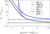 |
Fig. 2. Normalized pressure components, parallel Pi, ∥/PBM, ∥ (black) and perpendicular Pi, ⊥/PBM, ∥ (blue), and for BK (i = BK, dashed), RBK (i = RBK, solid), and BM (i = BM, dotted). |
3. Beaming distributions
Firstly, we consider the general situation when a beaming population, for example, electron strahl, exhibits an intrinsic pressure (or temperature) anisotropy, and later we particularize for isotropic temperatures. The anisotropic components of pressure (or temperature) show the same dependence on the model of velocity distribution, as already described above for non-drifting distributions, although in the solar wind frame (fixed to protons) the effective pressure (or temperature) is increased in parallel direction by the antisunward beaming speed (kBTeff = kBT + mV2). On the other hand, in this case we shall evaluate the higher order parameter giving the electron heat flux. The electron strahl, or beaming population, carries a significant amount of heat, which increases during (or after) the energetic events such as fast winds and CMEs, when the strahl relative density and beaming velocity may reach extreme values. However, the strahl also suffers a significant erosion with distance caused by a self-induced scattering triggered by the self-generated beam-plasma instabilities (Vocks et al. 2005; Maksimovic et al. 2005; Viñas et al. 2010; Verscharen et al. 2019; Tong et al. 2019). Values assumed in the present study for the relative densities and beaming velocities are in general relevant for various specific conditions in the solar wind, for example, slow or fast winds at various heliocentric distances.
3.1. Anisotropic temperatures
The electron strahl with anisotropic temperatures T∥ ≠ T⊥ can be reproduced by a drifting bi-κ-distribution (DBK) function (Nieves-Chinchilla & Viñas 2008; Viñas et al. 2010)given by
![$$ \begin{aligned} f_{\rm DBK}(v_\parallel , v_\perp ) = { n_0 \Gamma [\kappa ] \over (\pi \kappa )^{3/2} \theta _\parallel \theta _\perp ^2 \Gamma [\kappa -1/2]} \left(1 + \frac{(v_\parallel - V)^{2}}{\kappa \theta _\parallel ^2} + \frac{v_\perp ^{2}}{\kappa \theta _\perp ^2}\right)^{-\kappa -1}, \end{aligned} $$](/articles/aa/full_html/2020/02/aa36861-19/aa36861-19-eq16.gif)
where the beaming (drifting) velocity V is in parallel direction (along the magnetic field), and θ∥, ⊥ are given by the second order moments  . The same θ∥, ⊥ = (2kBTM, ∥, ⊥/m)1/2 describe the anisotropic beaming core within a drifting bi-Maxwellian (DBM)
The regularized DBK (RDBK) given by
![$$ \begin{aligned} f_{RDBK}(v_{\parallel }, v_\perp )&= {n_0 \;_{[0]}\mathcal{U} _{[]} \over (\pi \kappa )^{3/2}\theta _\parallel \theta _\perp ^2} \left(1 + \frac{(v_\parallel -V)^{2}}{\kappa \theta _\parallel ^2} + \frac{v_\perp ^{2}}{\kappa \theta _\perp ^2}\right)^{-\kappa -1} \nonumber \\&\quad \times \exp \left(- \frac{\alpha ^2 (v_\parallel -V)^{2}}{\theta _\parallel ^2} - \frac{\alpha ^2 v_\perp ^{2}}{\theta _\perp ^2}\right) \end{aligned} $$](/articles/aa/full_html/2020/02/aa36861-19/aa36861-19-eq19.gif)
combines a standard DBK with an exponential cutoff factor controlled by α < 1 (Scherer et al. 2019a). For α = 0 the RDBK reduces to a DBK, but, again, a finite value α > θ/c is required for the cutoff parameter in order to restrain to realistic speeds v < c (Scherer et al. 2019b). We use the general expression of the vector heat flux, for example, Eq. (6.5) in Paschmann et al. (1998)2, and derive the heat flux q = q∥ given by the strahl population along the magnetic field direction. It results from the general definition in statistical plasma physics (Paschmann et al. 1998) for the solar wind conditions, where the relative (counter-)drift of the central (core) population is in general very small, such that the suprathermal electron beaming populations remain the main contributor to the antisunward electron heat flux (Gary et al. 1999; Dudík et al. 2017). This is what we obtain, for a DBM,
see also Gary et al. (1999)3, for a DBK,
![$$ \begin{aligned} q_{\rm DBK} = {1 \over 2} n m_{\rm e} V \left[{\kappa \over \kappa -3/2} \left( {3 \over 2} \theta _\parallel ^2 + \theta _\perp ^2 \right)+ V^2 \right], \end{aligned} $$](/articles/aa/full_html/2020/02/aa36861-19/aa36861-19-eq21.gif)
and for a RDBK,
![$$ \begin{aligned} q_{\rm RDBK} = {1 \over 2} n m_{\rm e} V \left[ \kappa \, _{[2]}\mathcal{U} _{[0]}\left({3 \over 2} \theta _\parallel ^2 + \theta _\perp ^2 \right) + V^2 \right]. \end{aligned} $$](/articles/aa/full_html/2020/02/aa36861-19/aa36861-19-eq22.gif)
A comparison with previous results, for example, Eqs. (12) and (41) in Scherer et al. (2019a), suggests the existence of a typo affecting the contribution of perpendicular kinetic energy in their equations, but also the absence of the common factor 1/2, as resulting from their Eq. (7e) for the general definition of the heat flux2. Normalizing to Maxwellian limit, we find
and
![$$ \begin{aligned} {q_{\rm RDBK} \over q_{\rm DBM}} = {\left({3 \over 2} +A\right)\kappa \; _{[2]}\mathcal{U} _{[0]} + W^2 \over {3 \over 2} +A +W^2}, \end{aligned} $$](/articles/aa/full_html/2020/02/aa36861-19/aa36861-19-eq24.gif)
in terms of anisotropy  and normalized drift W = V/θ∥.
To evaluate the heat flux, we first consider  = 2 > 1, and temperatures characteristic to a hotter strahl T∥ = 3 105 K may be few times higher than temperature of central core+halo component (Viñas et al. 2010). The relative drift may vary with number density of beaming electrons. Thus, a low number density n1 = 0.02n0 and low beaming velocity W1 = V1/θ∥ = 0.5 can be specific to slow winds at low distances < 1 AU, or for any kind of slow or fast winds at large distances > 1 AU, as suggested in Maksimovic et al. (2005). In this case, for Maxwellian limit of the parallel (non-drifting) pressure, we find
  N m−2 and
  N m−2, while the heat flux, as given by Eq. (15), is qDBM ≃ 0.45 10−5 W m−2. The relative heat flux is plotted in Fig. 3, top panel, for both the DBK and RDBK distribution functions. For lower values of κ < 3/2 the heat flux may significantly increase up to, for example, qRDBK ≃ 0.25 10−3 W m−2 for κ = 1. A comparison can also be made for κ > 3/2, when, for instance, for κ = 1.6, we find qDBK ≃ 0.35 10−4 W m−2 and a reduced qRDBK ≃ 0.25 10−4 W m−2 (by minimizing the unrealistic contribution of superluminal particles with v > c).
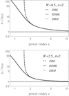 |
Fig. 3. Normalized heat flux for A = 2, W = 0.5 (top panel) and W = 2.5 (bottom panel), evaluated for DBK (i = DBK, dashed) and RDBK (i = RDBK, solid). |
More intense strahls with n2 = 0.1 n0 and W2 = V2/θ∥ = 2.5 are characteristic to fast winds at low distances < 1 AU (Maksimovic et al. 2005; Štverák et al. 2009). In the Maxwellian limit for the parallel component of the (non-drifting) pressure we find  N m−2 and
  N m2, while for the heat flux qDBM ≃ 0.3 10−3 W m−2. The relative heat flux is plotted in Fig. 3, bottom panel, for both the DBK and RDBK distribution functions, and for κ = 1 we find a higher heat flux qRDBK ≃ 0.7 10−2 W m−2. For κ = 1.6 we find a lower difference between qDBK ≃ 1.1 10−3 W m−2 and qRDBK ≃ 0.9 10−3 W m−2. In any of these cases, the heat flux decreases with increasing κ-index, i.e., with reducing the contribution of suprathermal or non-Maxwellian electrons in the strahl population. We note that for large κ → ∞ the strahl distribution reduces to a quasi-thermal Maxwellian representation, which should not be confused with the Maxwellian core in the central population of electrons observed in the solar wind.
In the opposite case, when the strahl exhibits a reversed anisotropy A = 0.1 < 1, we assume the same T∥ = 3 105 K and parallel pressure remains the same, but the heat flux may significantly change: see, for instance, Fig. 4, bottom panel. For less energetic strahls (W = 0.5), we obtain qDBM ≃ 0.23 10−5 W m−2, as given for reference by Eq. (15). The top panel of Fig. 4 shows the variation with κ of the relative heat flux, and both profiles for DBK and RDBK are similar to those obtained in Fig. 3 top panel. Thus, for κ < 1.5 the heat flux values remain much higher than those predicted for a BM; for example, for κ = 1 we find qRDBK ≃ 0.24 10−3 W m−2, while for κ = 1.6 qDBK ≃ 0.35 10−4 W m−2 and qRDBK ≃ 0.25 10−4 W m−2 is slightly reduced. The situation is much different for more energetic beams with W = 2.5 (bottom panel) when qDBM ≃ 0.05 10−3 W m−2 and values obtained for the heat flux in the limit of very small values of κ → 1 may be one order of magnitude lower than that obtained in top panel; this also highly contrasts with the corresponding result in Fig. 3, bottom panel. In this case, for κ = 1 we find qRDBK ≃ 0.7 10−2 W m−2, while for κ = 1.6 we get qDBK ≃ 1.6 10−3 W m−2 and qRDBK ≃ 0.12 10−3 W m−2.
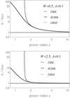 |
Fig. 4. Normalized heat flux for A = 0.1, W = 0.5 (top panel) and W = 2.5 (bottom panel), evaluated for DBK (i = DBK, dashed) and RDBK (i = RDBK, solid). |
3.2. Isotropic temperatures
If the temperature of beaming population is (almost) isotropic, i.e., T∥ ≃ T⊥, the heat flux can be calculated (for A = 1) using the same expressions (15)–(17) for their absolute values or (18)–(19) for their relative values. Profiles of the (relative) heat-flux dependence on κ are shown in Fig. 5 and are very similar to those obtained in Fig. 3. Values provided for the heat flux by the standard κ-distribution and by the regularized model are also comparable with those obtained for A = 2. The contrast should increase for higher anisotropies A ≫ 1.
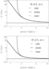 |
Fig. 5. Normalized heat flux for A = 1, W = 0.5 (top panel) and W = 2.5 (bottom panel), evaluated for DBK (i = DBK, dashed) and RDBK (i = RDBK, solid). |
4. Discussion and conclusions
A macroscopic description of collisionless plasmas out of thermal equilibrium is not always straightforward because it is highly dependent on the model function describing the velocity distribution of plasma particles. For κ-distribution functions a macroscopic description is simply altered by the divergence of higher order moments, such as temperature, pressure, or heat flux, for plasma states with significant suprathermal populations. For that reason the distributions with hard suprathermal tails are discarded from the observational analysis. In the absence of relativistic corrections, moments of standard κ-distributions may also include unphysical contributions of superluminal particles with speeds larger than the speed of light in vacuum.
Regularized κ-distribution (RK) functions (Scherer et al. 2017) were introduced to overcome these limitations, and in this work we invoked these models to evaluate the pressure and heat flux of electron populations for solar wind conditions at 1 AU. The heat-flux values summarized in Tables 1 and 2 and discussed in the previous section are all in the range of the electron heat flux measured in the solar wind by different missions, from very early Imp 6, 7, or 8, to Ulysses and Wind spacecraft (Feldman et al. 1975; Cuperman 1980; Scime et al. 2001; Pagel et al. 2005). Of particular interest are plasma states dominated by the suprathermal populations, for example, for κ < 2, when the pressure or the heat flux transported by the beaming populations may be at least one order of magnitude higher than estimates made by ignoring suprathermal populations. In this case, the corresponding moments obtained for a standard κ-distribution are defined only for κ > 3/2 and can markedly overestimate predictions made by the RKs. We have to point out that values chosen for the cutoff parameter α may have various motivations; for example, for RR < 1% Scherer et al. (2019b) have considered reducing the unrealistic effects of superluminal particles to a reasonably acceptable level. With the parameters adopted in our study this condition may indeed let α be closer to θ/c ≃ 0.005, than our alternative α = 0.012 that rather reduces the implications of superluminal particles. For slightly higher values of α our results move toward a Maxwellian prediction, while lower values increase the effects of suprathermals, especially for κ ≤ 2. Other constraints on the α value may be introduced by the observational spectra showing dropping shoulders, as an indication of different populations present at higher energies but with lower intensities.
Heat flux (W m−2) for A = 2.
Heat flux (W m−2) for A = 0.1.
We can conclude trusting that based on the RK model functions, a realistic and physically well-defined parametrization becomes possible even for collisionless plasmas with various nonthermal features such as suprathermal populations or kinetic anisotropies. Values derived in this work for macroscopic properties of RK electrons (either isotropic or anisotropic) can be confronted with those obtained from a direct numerical integration of observational data (Paschmann et al. 1998). Once accurately estimated, these parameters can be used as initial conditions as well as boundary conditions, for example, in plasma transport models for the evolution of the expanding solar wind in heliosphere (Pierrard et al. 2001, 2011) and for its interaction with planetary atmospheres.
Comparison with the corresponding pressures in Scherer et al. (2019b) suggests a typo in their Eqs. (5)–(7), where the factor 3/2 must be replaced by 1/2.
Equation (7e) in Scherer et al. (2019a) differs by a factor of 1/2 and is not consistent with the definition (mv2/2) used in our paper for the kinetic energy of plasma particles.
This expression is also adopted in Gary et al. (1999), even though it is not consistent with their definition (mv2) for the kinetic energy of plasma particles.
Acknowledgments
KS and HF are grateful to the Deutsche Forschungsgemeinschaft, DFG funding the projects SCHE334/10-1, respectively. ML acknowledges support in the framework of the projects G0A2316N (FWO–Vlaanderen) and SCHL 201/35-1 (DFG). The authors also acknowledge fruitful discussions within the ISSI team on Kappa Distributions hosted by the International Space Science Institute (ISSI) in Bern.
References
- Collier, M. R., Hamilton, D. C., Gloeckler, G., Bochsler, P., & Sheldon, R. B. 1996, Geophys. Res. Lett., 23, 1191 [NASA ADS] [CrossRef] [Google Scholar]
- Cuperman, S. 1980, Space Sci. Rev., 26, 277 [NASA ADS] [CrossRef] [Google Scholar]
- Dudík, J., Dzifčáková, E., Meyer-Vernet, N., et al. 2017, Sol. Phys., 292, 100 [NASA ADS] [CrossRef] [Google Scholar]
- Feldman, W. C., Asbridge, J. R., Bame, S. J., Montgomery, M. D., & Gary, S. P. 1975, J. Geophys. Res., 80, 4181 [NASA ADS] [CrossRef] [Google Scholar]
- Gary, S. P., Skoug, R. M., & Daughton, W. 1999, Phys. Plasmas, 6, 2607 [NASA ADS] [CrossRef] [Google Scholar]
- Lazar, M., Poedts, S., & Fichtner, H. 2015, A&A, 582, A124 [NASA ADS] [CrossRef] [EDP Sciences] [Google Scholar]
- Lazar, M., Fichtner, H., & Yoon, P. H. 2016, A&A, 589, A39 [NASA ADS] [CrossRef] [EDP Sciences] [Google Scholar]
- Lazar, M., Pierrard, V., Shaaban, S. M., Fichtner, H., & Poedts, S. 2017, A&A, 602, A44 [NASA ADS] [CrossRef] [EDP Sciences] [Google Scholar]
- Leubner, M. P., & Vörös, Z. 2005, Nonlinear Processes Geophys., 12, 171 [NASA ADS] [CrossRef] [Google Scholar]
- Maksimovic, M., Pierrard, V., & Lemaire, J. F. 1997, A&A, 324, 725 [NASA ADS] [Google Scholar]
- Maksimovic, M., Zouganelis, I., Chaufray, J.-Y., et al. 2005, J. Geophys. Res. (Space Phys.), 110, A09104 [NASA ADS] [CrossRef] [Google Scholar]
- Meyer-Vernet, N. 2001, Science, 49, 247 [Google Scholar]
- Nicholls, D. C., Dopita, M. A., & Sutherland, R. S. 2012, ApJ, 752, 148 [NASA ADS] [CrossRef] [Google Scholar]
- Nieves-Chinchilla, T., & Viñas, A. F. 2008, J. Geophys. Res. (Space Phys.), 113, A02105 [NASA ADS] [CrossRef] [Google Scholar]
- Pagel, C., Crooker, N. U., & Larson, D. E. 2005, Geophys. Res. Lett., 32 [Google Scholar]
- Paschmann, G., Fazakerley, A. N., & Schwartz, S. J. 1998, ISSI Sci. Rep. Ser., 1, 125 [NASA ADS] [Google Scholar]
- Pierrard, V., & Lazar, M. 2010, Sol. Phys., 267, 153 [NASA ADS] [CrossRef] [Google Scholar]
- Pierrard, V., Lazar, M., & Schlickeiser, R. 2011, Sol. Phys., 269, 421 [NASA ADS] [CrossRef] [Google Scholar]
- Pierrard, V., Maksimovic, M., & Lemaire, J. 2001, J. Geophys. Res., 106, 29305 [Google Scholar]
- Scherer, K., Fichtner, H., & Lazar, M. 2017, Europhys. Lett., 120, 50002 [NASA ADS] [CrossRef] [Google Scholar]
- Scherer, K., Lazar, M., Husidic, E., & Fichtner, H. 2019a, ApJ, 880, 118 [NASA ADS] [CrossRef] [Google Scholar]
- Scherer, K., Fichtner, H., Fahr, H. J., & Lazar, M. 2019b, ApJ, 881, 93 [NASA ADS] [CrossRef] [Google Scholar]
- Scime, E. E., Littleton, J. E., Gary, S. P., Skoug, R., & Lin, N. 2001, Geophys. Res. Lett., 28, 2169 [NASA ADS] [CrossRef] [Google Scholar]
- Scudder, J. D. 1992, ApJ, 398, 319 [NASA ADS] [CrossRef] [Google Scholar]
- Tong, Y., Vasko, I. Y., Pulupa, M., et al. 2019, ApJ, 870, L6 [NASA ADS] [CrossRef] [Google Scholar]
- Treumann, R. A., Jaroschek, C. H., & Scholer, M. 2004, Phys. Plasmas, 11, 1317 [NASA ADS] [CrossRef] [Google Scholar]
- Vasyliunas, V. M. 1968, J. Geophys. Res., 73, 2839 [NASA ADS] [CrossRef] [Google Scholar]
- Verscharen, D., Chandran, B. D. G., Jeong, S.-Y., et al. 2019, ApJ, 886, 2 [CrossRef] [Google Scholar]
- Viñas, A. F., Gurgiolo, C., Nieves-Chinchilla, T., Gary, S. P., & Goldstein, M. L. 2010, in Twelfth International Solar Wind Conference, eds. M. Maksimovic, K. Issautier, N. Meyer-Vernet, M. Moncuquet, & F. Pantellini, Am. Inst. Phys. Conf. Ser., 1216, 265 [NASA ADS] [Google Scholar]
- Vocks, C., Salem, C., Lin, R. P., & Mann, G. 2005, APJ, 627, 540 [Google Scholar]
- Štverák, Š., Maksimovic, M., Trávníček, P. M., et al. 2009, J. Geophys. Res. (Space Phys.), 114, A05104 [NASA ADS] [Google Scholar]
- Štverák, Š., Trávníček, P., Maksimovic, M., et al. 2008, J. Geophys. Res., 113, A03103 [Google Scholar]
Appendix A: Abbreviations
The abbreviations used for various distribution functions are explained and summarized below in Tables A.1 and A.2.
Non-drifting distributions.
Drifting (or beaming) distributions (apply for both cases of anisotropic or isotropic temperatures, see Sect. 3).
All Tables
Drifting (or beaming) distributions (apply for both cases of anisotropic or isotropic temperatures, see Sect. 3).
All Figures
|
Fig. 1. Normalized pressure Pi/PM for a standard (isotropic) κ-distribution (i = K, red dashed) and for the regularized κ-distribution (i = RK, black solid) in bottom panel with a zoom-in only for a restraint range of conditions relevant for the solar wind. |
| In the text | |
|
Fig. 2. Normalized pressure components, parallel Pi, ∥/PBM, ∥ (black) and perpendicular Pi, ⊥/PBM, ∥ (blue), and for BK (i = BK, dashed), RBK (i = RBK, solid), and BM (i = BM, dotted). |
| In the text | |
|
Fig. 3. Normalized heat flux for A = 2, W = 0.5 (top panel) and W = 2.5 (bottom panel), evaluated for DBK (i = DBK, dashed) and RDBK (i = RDBK, solid). |
| In the text | |
|
Fig. 4. Normalized heat flux for A = 0.1, W = 0.5 (top panel) and W = 2.5 (bottom panel), evaluated for DBK (i = DBK, dashed) and RDBK (i = RDBK, solid). |
| In the text | |
|
Fig. 5. Normalized heat flux for A = 1, W = 0.5 (top panel) and W = 2.5 (bottom panel), evaluated for DBK (i = DBK, dashed) and RDBK (i = RDBK, solid). |
| In the text | |
Current usage metrics show cumulative count of Article Views (full-text article views including HTML views, PDF and ePub downloads, according to the available data) and Abstracts Views on Vision4Press platform.
Data correspond to usage on the plateform after 2015. The current usage metrics is available 48-96 hours after online publication and is updated daily on week days.
Initial download of the metrics may take a while.