| Issue |
A&A
Volume 628, August 2019
|
|
|---|---|---|
| Article Number | A111 | |
| Number of page(s) | 6 | |
| Section | Stellar atmospheres | |
| DOI | https://doi.org/10.1051/0004-6361/201936011 | |
| Published online | 14 August 2019 | |
The 6Li/7Li isotopic ratio in the metal-poor binary CS22876–032★,★★
1
Instituto de Astrofísica de Canarias,
Vía Láctea,
38205 La Laguna,
Tenerife, Spain
e-mail: jonay@iac.es
2
Departamento de Astrofísica, Universidad de La Laguna,
38206 La Laguna,
Tenerife, Spain
3
GEPI, Observatoire de Paris, Université PSL, CNRS,
5 Place Jules Janssen,
92190 Meudon, France
4
Zentrum für Astronomie der Universität Heidelberg, Landessternwarte,
Königstuhl 12,
69117 Heidelberg, Germany
5
Leibniz-Institut für Astrophysik Potsdam (AIP),
An der Sternwarte 16,
14482 Potsdam, Germany
6
Departamento de Ciencias Fisicas, Universidad Andres Bello,
Fernandez Concha 700,
Las Condes, Santiago, Chile
Received:
3
June
2019
Accepted:
10
July
2019
Aims. We present high-resolution and high-quality UVES spectroscopic data of the metal-poor double-lined spectroscopic binary CS 22876–032 ([Fe/H] approximately −3.7 dex). Our goal is to derive the 6Li/7Li isotopic ratio by analysing the Li I λ 670.8 nm doublet.
Methods. We co-added all 28 useful spectra normalised and corrected for radial velocity to the rest frame of the primary star. We fitted the Li profile with a grid of the 3D non-local thermodynamic equilibrium (NLTE) synthetic spectra to take into account the line profile asymmetries induced by stellar convection, and performed Monte Carlo simulations to evaluate the uncertainty of the fit of the Li line profile.
Results. We checked that the veiling factor does not affect the derived isotopic ratio, 6 Li/7Li, and only modifies the Li abundance, A(Li), by about 0.15 dex. The best fit of the Li profile of the primary star provides A(Li) = 2.17 ± 0.01 dex and 6 Li/7Li = 8−5+2% at 68% confidence level. In addition, we improved the Li abundance of the secondary star at A(Li) = 1.55 ± 0.04 dex, which is about 0.6 dex lower than that of the primary star.
Conclusions. The analysis of the Li profile of the primary star is consistent with no detection of 6 Li and provides an upper limit to the isotopic ratio of 6 Li/7Li < 10% at this very low metallicity, about 0.5 dex lower in metallicity than previous attempts for detection of 6 Li in extremely metal poor stars. These results do not solve or worsen the cosmological 7 Li problem, nor do they support the need for non-standard 6Li production in the early Universe.
Key words: stars: Population II / stars: individual: CS22876–032 / Galaxy: abundances / Galaxy: halo / cosmology: observations / primordial nucleosynthesis
The two averaged spectra are only available at the CDS via anonymous ftp to cdsarc.u-strasbg.fr (130.79.128.5) or via http://cdsarc.u-strasbg.fr/viz-bin/qcat?J/A+A/628/A111
© ESO 2019
1 Introduction
The standard Big Bang nucleosynthesis (SBBN) theory predicts a very small primordial production of lithium in the first minutes of the Universe, at about ten orders of magnitude lower than H and He (e.g. Steigman 2007; Cyburt et al. 2016). This prediction mainly depends on the density of baryons inferred from the fluctuations of the cosmic microwave background (CMB) as measured by the Wilkinson Microwave Anisotropy Probe (WMAP; Spergel et al. 2007) and the Planck satellite (Planck Collaboration XIII 2016). This small amount of Li predicted, ranging from A(7 Li)1 = 2.67 (Cyburt et al. 2016) to 2.74 (Coc & Vangioni 2017), is still a factor of three greater than the almost uniform measured Li content in the atmosphere of unevolved metal-poor field stars (e.g. Spite & Spite 1982; Rebolo et al. 1988; Bonifacio et al. 2007a; Aoki et al. 2009) or in globular clusters (e.g. Bonifacio et al. 2007b; González Hernández et al. 2009).
A variety of different models have been proposed to try to explain this abundance difference known as the cosmological lithium problem (see e.g. Fields et al. 2014, and references therein). However, more recent studies have shown a decline and/or an increasing scatter in the Li abundances in metal-poor stars for metallicities [Fe/H] < −3 (e.g. Sbordone et al. 2010; Bonifacio et al. 2012; Matsuno et al. 2017). In particular, the flame of the cosmological Li problem has recently been relighted with the Li detection in some extremely iron-poor stars (Hansen et al. 2014; Starkenburg et al. 2018; Bonifacio et al. 2018; Aguado et al. 2019), in contrast with the Li non-detections in apparently similar stars (Frebel et al. 2005; Caffau et al. 2011; Bonifacio et al. 2015). Two extremely iron-poor stars, SDSS J0135+0641 (Bonifacio et al. 2015, 2018) at [Fe/H] < −5.2, and SDSS J0023+0307 (Aguado et al. 2018, 2019) at [Fe/H] < −6.1, almost recover the level of the lithium plateau, with lithium abundances of A(Li) ~ 1.9 and ~ 2.0, respectively. These recent discoveries pose strong constraints on any theory aiming to explain the cosmological Li problem.
The SBBN prediction for the 6Li isotope is even lower, at about A(6Li) approximately − 1.9 (Cyburt et al. 2016), i.e. a tiny isotopic ratio of 6Li ∕ 7Li = 2.75 × 10⁻⁵, not measurable through spectral analysis of stars. However, 6Li, like the B and Be isotopes, can be efficiently produced by the interaction of energetic nuclei of Galactic cosmic rays (GCR) with the nuclei of the interstellar medium (ISM), where the 6 Li abundance should increase as the metallicity increases (Prantzos 2012). The predicted level of the isotopic ratio 6Li ∕ 7Li is 1% at metallicity [Fe/H] = −2. Detecting higher amounts of 6Li at low metallicities may suggest other production channels, for example non-standard physics in the Big Bang (Jedamzik & Pospelov 2009), or a pre-galactic origin (Rollinde et al. 2006).
The presence of 6Li in metal-poor halo stars can only be derived from the asymmetry in the red wing of the 7 Li doublet line at λ 670.8 nm. The treatment ofthis line using 1D model atmospheres and local thermodynamical equilibrium (LTE) spectral synthesis produced presumably the detection of 6Li in several stars at [Fe/H] < −2 (Cayrel et al. 1999; Asplund et al. 2006). However, convective flows in the atmospheres of metal-poor stars are likely responsible for part of this asymmetry (Cayrel et al. 2007). The re-analysis of the Li feature, using 3D hydrodynamical models and a 3D-NLTE treatment, in some metal-poor stars was not able to confirm the detection of 6 Li (Steffen et al. 2012; Lind et al. 2013).
The metal-poor spectroscopic binary CS 22876–032, with very low metallicity at about [Fe/H] approximately − 3.7 (Molaro & Castelli 1990; Norris et al. 2000; González Hernández et al. 2008), and its relatively large brightness (mV = 12.8), provide a unique opportunity to search for 6Li in the primary star using high-resolution spectroscopic observations and 3D-NLTE synthetic profiles. Here we report on the search for 6 Li in CS 22876–032, and therefore a test performed at about 0.5 dex lower metallicity than other previous attempts to detect 6 Li in extremely metal-poor stars. The Li abundances of both binary stellar components have been already reported, but only the primary star has a Li abundance at the level of the Spite plateau (González Hernández et al. 2008).
2 Observations and data analysis
We carried out spectroscopic observations with UVES at UT2/VLT in Paranal (Chile) using the image slicer #3 on 2007 October 17, 18, 19, and 20. These dates were adequate since the orbital phase of the binary was ~ 0.67 where both stellar components were close to the maximum line-of-sight radial velocity difference (see Fig. 1). Another single observation with the same configuration was acquired on 2007 December 07 (with a median S ∕ N ~ 67 per order), but was discarded in this analysis since it shows a different orbital phase with both stellar components closer in radial velocity. We obtained 28 useful observations of 3600 s, covering the spectral region λλ495.95–707.08 nm at a resolving power R ~ 107 200. The reduced spectra were downloaded from the ESO Archive Science Portal. The median signal-to-noise ratio (S/N) per order is in the range 55–75, except for three spectra with a S ∕ N ~ 32, 37, and 50 with shorter exposure times of ~1890 s, 2160 s, and 2500 s. The individual reduced order-merged spectra were first normalised in the whole wavelength range with a fifth-order polynomial using our own automated IDL-based routine and then corrected for barycentric velocity. Radial velocities (RV) were obtained by cross-correlating each spectrum with a mask centred at the Mg Ib triplet lines and modelled using a Gaussian with the full width half maximum (FWHM) equal to the resolving power (FWHM = 2.8 km s−1, R ~ 107 200) of the observed spectrum and contrast equivalent to relative depths of the Mg Ib triplet lines in the primary (star A).
In Fig. 1 we show the RV curve of the two stellar components, with the RVs of the primary and the secondary at about RVA = −80.4 ± 0.2 km s−1 and RVB = −106.3 ± 0.6 km s−1 during those nights. We compute the weighted RV average for each night and fit these RV points together with those in González Hernándezet al. (2008, and references therein) using the RVFIT tool (Iglesias-Marzoa et al. 2015) to update the orbital parameters of the binary shown in Table 1.
The individual spectra normalised to unity were corrected for the RV of star A and co-added all together. Only a small fraction of flux points, deviating more that 2σ from the mean flux, were discarded. In Fig. 2 we show a small portion, the Mg 1b triplet spectral region, of the normalised, co-added spectrum in the rest frame of the primary (star A). The S/N of this spectrum at continuum surrounding the Mg Ib triplet is S ∕ N ~ 100. Finally, we rebinned the co-added spectrum with a wavelength step of 0.014 Åpixel−1, by taking the weighted (by flux errors) mean of the flux points and respective wavelengths of each bin, providing a S∕N ~ 570 at the continuum (see Fig. 2). The spectral lines of each binary component appear weakened because of the veiling (fA = 1.33 and fB = 4.03 at the Mg Ib triplet) that each star produces on the flux of the other component (see González Hernández et al. 2008, for more details on the determination of veiling factors in this binary system).
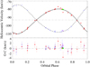 |
Fig. 1 Radial velocities of the primary (star A: filled symbols) and the secondary (star B: open symbols) of CS 22876–032 (upper panel), and residuals from the fit (lower panel). Triangles and circles are literature (Norris et al. 2000; González Hernández et al. 2008) and new UVES observations, respectively. The curves show the orbital solution (see Table 1) for star A (solid) and B (dashed). Triple dotted-dashed horizontal line shows the centre-of-mass velocity of the system. |
Updated orbital elements of CS 22876–032.
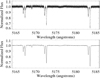 |
Fig. 2 Normalised, co-added, RV-corrected, unveiled spectrum of CS 22876–032 shown in the spectral region of the Mg Ib triplet (upper panel) and rebinned to a wavelength step of 0.014 Å pixel−1 (lower panel) in the rest frame of star A. |
3 3D model atmospheres and non-LTE spectrum synthesis
The lithiumabundance and isotopic ratio are derived by fitting synthetic line profiles of the Li I λ 670.8 nm doublet to the observed spectrum. Synthetic spectra are computed from 3D hydrodynamical CO5BOLD model atmospheres and account for 3D non-LTE effects.
The 3Dmodel atmosphere chosen for the primary has a temporal average effective temperature 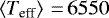 K, surface gravity log g = 4.5, and metallicity [Fe/H] = −4. The atmosphere of the secondary is represented by a 3D model with
  K, log g = 4.5, and [Fe/H] = −4. The non-local radiative transfer is solved in 12 opacity bins on a standard grid of 140 × 140 × 150 cells (see Ludwig et al. 2009, for further details on the 3D hydrodynamical model atmospheres). To reduce the burden of computing the synthetic line profiles, a number of representative snapshots were selected from the full time sequence of the two simulations (19 for the hotter model and 20 for the cooler).
As an intermediate step, the non-LTE departure coefficients bi = ni(NLTE) ∕ ni(LTE) for each level i of the 17 level lithium model atom with 34 line transitions were computed as a function of geometrical position within all selected 3D model atmospheres (see e.g. Steffen et al. 2012; Klevas et al. 2016; Mott et al. 2017, for details on the lithium model atom and the 3D-NLTE treatment). Since the Li resonance line is weak, the departure coefficients are essentially independent of the assumed Li abundance within the considered range.
For both binary components, we then created a grid of 3D non-LTE synthetic spectra of the Li I λ 670.8 nm doublet for different Li abundances and isotopic ratios. The synthetic line profiles are computed with the line formation code LINFOR3D2, taking into account the detailed 3D thermal structure and hydrodynamical velocity field of the selected snapshots and using the previously computed NLTE departure coefficients.
4 Lithium profile of the primary star
The co-added spectrum in the rest frame of the primary star A is shown in Fig. 3 for the spectral range λλ670.6−670.9 nm. We used this spectrum without rebinning to measure the lithium isotopic ratio in the primary star. The large number of co-added spectra allowed us to perform the fit of the Li feature including about 1100 line flux points and 1160 continuum flux points in the spectral range λλ670.6−670.9 nm. The spectral lines of each binary component appeared weaker due to the corresponding veiling at the Li I doublet spectral region. We corrected for the veiling at the Li 1 doublet spectral region with the factors fA = 1.36 and fB = 3.74, for the primary and secondary respectively (González Hernández et al. 2008).
The grid was created for three different values of Li abundance (A(Li) = 1.6, 2.0 and 2.4), isotopic ratio (6 Li/7Li = 0, 4 and 8%), and global broadening (vBR = 0, 4.5 and 9 km s−1), modelled as a Gaussian accounting for instrumental broadening, vINS, and rotational broadening, vROT. We performed a fit of the unbinned Li profile of the primary using an automated IDL-based routine that makes use of the MPFIT3 routine (Markwardt 2009), including five free parameters: continuum location, global Gaussian broadening, velocity shift, lithium abundance, and isotopic ratio. We allowed the fitting procedure to also explore negative values of vBR, down to −5 km s−1, by extrapolating in the grid of synthetic Li profiles. The fitting procedure provides essentially the same 6 Li/7Li isotopic ratio for the unveiled and veiled spectrum of the primary star, but the Li abundance is lower by about 0.15 dex for the veiled spectrum. We therefore decided to run the fitting procedure on the unveiled spectrum. In Fig. 3 we show the best fit of the unbinned Li profile of star A, which gives 6 Li/7Li = 7.9 ± 8.2%, A(Li) ~ 2.17 ± 0.02 dex, vBR = 1.1 ± 3.4 km s−1, and a global velocity shift of the line profile consistent with zero within the error bars. A S∕N ~ 74 is inferred from the scatter of the fit residuals.
To evaluate the uncertainty on Li abundance and isotopic ratio we ran 10 000 Monte Carlo simulations by injecting Poisson noise in the best fit according to the S/N at the continuum level of the unbinned spectrum. We then repeated our fitting procedure 10 000 times, replacing the observed spectrum by each of the resulting 10 000 artificial realisations. In Fig. 4 we show the distribution of the 10 000 Monte Carlo simulations of the lithium isotopic ratio versus the broadening velocity vBR. There is a clear correlation between the isotopic ratio and the broadening velocity. The projection of these simulations over broadening velocity shows a symmetric distribution and provides the same value as the single best fit: vBR = 1.1 ± 1.8 km s−1. This value is lower than the instrumental broadening (vINS ~ 2.8 km s−1), which points to a too broad CO5BOLD 3D-NLTE line profile that needs to be further investigated. In Fig. 5 we show the distributions of the Monte Carlo simulations for lithium isotopic ratio versus the lithium abundance. About 30% of the simulations fall at vBR < 0 km s−1 and 6 Li/7Li 0, which were discarded in Fig 5. Most of the remaining simulations fall at the same values of the initial best fit and the contours and density distributions of Li abundance and isotopic ratio provide the same answer: 6 Li/7Li  % and A(Li) ~ 2.17 ± 0.01 dex. This defines an upper limit to the isotopic ratio of 6 Li/7Li < 10.2 and 13.8% at 1σ and 2σ confidence, respectively.
In Fig. 6 we show the unveiled Li profile of the primary star rebinned with a wavelength step of 0.014 Å pixel−1. The fit of the rebinned spectrum provides a similar result, within the error bars, to that of the unbinned co-added spectrum, as expected (Bonifacio 2005), but the result obtained using the unbinned spectrum is statistically more robust. The number of fitted points in the rebinned case are 50 and 54 for the line and continuum, and we get a S∕N ~ 422 from the residuals of the fit. From this best fit we measure the EW of the Li profile of the primary star at 17.0 ± 0.3 mÅ.
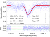 |
Fig. 3 Normalised, co-added, RV-corrected, unveiled spectrum of CS 22876–032A (blue dots), together with best-fit 3D-NLTE Li profile (red circles), and residuals of the fit (lower panel). The mean flux uncertainty is shown on the right as a blue circle with error bars. The horizontal dashed and dot-dashed lines indicate the 1σ dispersion of the observed flux points relative to the mean difference observed minus computed profiles. |
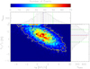 |
Fig. 4 Density distributions of lithium isotopic ratio vs. broadening velocity of 10 000 Monte Carlo simulations to evaluatethe confidence of the best fit to the Li profile of star A. The green dash-dotted lines indicate the 1σ uncertainty,whereas the blue dotted and red dashed lines are the best fit values and the centre of the distributions, respectively. |
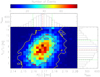 |
Fig. 5 Same as Fig. 4, but for the lithium isotopic ratio vs. lithium abundance. About 70% of the simulations shown here fall at vBR ≥ 0 and 6 Li/7Li ≥ 0. |
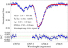 |
Fig. 6 Best fit (red circles) to the unveiled Li profile of star A (blue circles) rebinned to a wavelength step of 0.014 Å pixel−1 (upper panel) and the residuals of the fit (lower panel). |
5 Lithium profile of the secondary star
The RV corrected, rebinned, unveiled spectrum in the rest frame of the secondary is shown in Fig. 7. The 3D-NLTE grid was created for the A(Li) = 1.4, 1.8, and 2.2 based on the 3D hydrodynamical model with 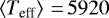 K, log g = 4.5, and Fe/H] = −4. We fit in this case 44 line points and 62 continuum points of the observed Li profile of the secondary, using the same automated routine as before, but fixing the isotopic ratio at 6 Li/7Li = 0% and the global broadening to the instrumental resolution at vBR = 2.8 km s−1. We fit in this case 44 line points and 62 continuum points and extract a S ∕ N ~ 149 from the residuals. The best fit givesA(Li) = 1.55 ± 0.04 dex and an EW(Li) = 10.9 ± 0.8 mÅ. The global shift of the best fit is a bit large, but still acceptable according to the errors on the individual RVs of star B. This is a downward revision the Li abundance of the secondary by 0.22 dex relative to the 1D NLTE Li abundance of A(Li) = 1.77 given in González Hernández et al. (2008) and is consistent with the higher quality data presented in the present work.
6 Discussion and conclusions
The Li abundance of the secondary appears to be significantly lower than that of the primary, by about 0.6 dex. This result strengthens the increased scatter of Li abundances in unevolved metal-poor stars with [Fe/H] < −3.5 dex. This increased scatter and possibly meltdown of the Li plateau at the lowest metallicities (Sbordone et al. 2010) is also consistent with the similar Li abundance at roughly the level of the Li plateau (A(Li)A-B = 0.1 dex) for both components (with Teff,A = 6350 K and Teff,B = 5830 K) of the doubled-line spectroscopic binary G166–45 at a metallicity [Fe/H] = −2.5 (Aoki et al. 2012). These authors discussed it in the context of the mass-dependent Li depletion suggested by Meléndez et al. (2010), which does not seem to be supported by the Li abundances of these two spectroscopic binaries.
In Figs. 8 and 9 we compare the Li abundances of star A and B of CS 22876–032 with the literature measurements for stars with [Fe/H] ≤ −3.0 and logg > 3, showing the meltdown of the lithium plateau (Sbordone et al. 2010). In this metallicity regime, most of the stars are located around A(Li) ~ 2.0 and there is an evident lack of stars between this upper envelope defined by the lithium plateau and the predicted SBBN primordial Li abundance. This is clearly seen if we only consider the measurements; leaving aside the upper limits, there appears to be a trend of Li abundance with effective temperature, together with increasing scatter towards lower temperatures. This trend is expected as a result of convection being stronger in cooler stars, thus resulting in stronger Li depletion. What is not expected is that the Li depletion begins at such warm effective temperatures at Teff ~ 6100 K. At metallicities [Fe/H] approximately −2 the same pattern happens at Teff ~ 5800 K (Bonifacio & Molaro 1997). Based on this evidence Bonifacio et al. (2018) have suggested that the Li depletion starts at increasingly higher effective temperatures with decreasing metallicity. The binary CS 22876–032 provides strong support to this claim since the two stars should have formed with the same Li abundance.
The Li upper limits complicate the picture since some are found at very high effective temperatures. The stars with Teff > 6500 K and no Li detected are SDSS J150702+005152 (Bonifacio et al. 2018), and HE 1029-0546 and HE 1241-2907 (Hansen et al. 2015). Ryan et al. (2001) have suggested that the stars with no measurable Li are future blue-stragglers and that the absence of Li in these stars is the result of the merging of two main-sequence stars that form the blue straggler. Bonifacio et al. (2019) have shown that three of the four stars studied by Ryan et al. (2001) are indeed canonical blue stragglers. This suggests a simple interpretation of Fig. 8 and the meltdown of the Spite plateau (see also Fig. 9): all stars with no measurable Li are blue stragglers or blue-stragglers-to-be, while all stars with measurable Li were formed with a Li abundance equal to the Spite plateau value, and the cooler stars underwent depletion due to convection. This hypothesis would be disproved if any of the upper limits at A(Li) < 1.5 were turned into an actual measurement. A blue straggler has no measurable Li.
Another way to probe the effects of convection in the stars of this system is to measure the Be abundance in the two stars. Ifconvection has been so vigorous to substantially deplete Li in CS 22876–032 B, it may also have been able to deplete Be and thus the two stars would also have different Be abundances. However, regarding Be, the picture might be considerably more complex. González Hernández et al. (2008) found an upper limit log(Be/H) < −13.0 and we concluded that since this was one order of magnitude higher than expected for stars at this metallicity it was not significant. We overlooked the fact that the star is highly enhanced in oxygen and thus we should compare this Be upper limit with the Galactic Be-O trend. CS 22876-32 A has [O/H] = –1.56 in 1D LTE (we assumed a solar oxygen abundance 8.76 from Steffen et al. 2015). If we consider thestraight line fit to the 1D LTE data of Boesgaard et al. (2011) we find that for this oxygen abundance we expect log(Be/H) = −12.74. Thus, our upper limit is marginally significant, we should have measured Be. It could simply be that this system is one that significantly deviates from the Galactic Be-O relation. Spite et al. (2019) found that 2MASS J1808-5104, which has a similar [Fe/H] but lower [O/H] than CS 22876-32, has no detectable Be and its upper limit lies well below the Galactic Be-O line. Another similar case is the CEMP-no star BD +44° 493 (Ito et al. 2013), again a similar [Fe/H] and no detectable Be. Both stars appear in Fig. 8 at the lowest Teff and are Li depleted, but with measurable Li. The explanation suggested by Spite et al. (2019) for these stars was that their age is old enough that cosmic rays did not have enough time to build significant quantities of Be. New higher-quality observations of Be in CS 22876-32 would be very valuable, since they would allow us to establish if this system lies on the Galactic Be-O line or if it is below the line, like 2MASS J1808-5104 and BD +44° 493.
The analysis of the high-quality UVES spectrum of the metal-poor binary CS 22876-032 using 3D-NLTE synthetic spectra of the Li I λ670.8 nm doublet does not provide a strong detection of the 6Li isotope. The results of the primary star can be interpreted as an upper limit of the Li isotopic ratio of the 6 Li/7Li < 10%. However, the result is also consistent with no detection of 6 Li. This together with the upper limits and/or non-detections of 6Li in other single metal-poor stars (Steffen et al. 2012; Lind et al. 2013) when a 3D-NLTE analysis is performed seem to solve the so-called second cosmological Li problem, and therefore support the negligible amount of 6 Li predicted in standard Big Bang nucleosynthesis models. Future observations performed with the ESPRESSO spectrograph at the 8.2 m VLT (e.g. Pepe et al. 2014; González Hernández et al. 2018) using the UHR mode at R ~ 200 000 with a pixel size of 0.5 km s−1 and fiber diameter of 0.5 arcsec may help to further investigate the lithium isotopic ratio and velocity fields of these and other metal poor stars.
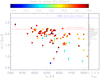 |
Fig. 8 Lithium abundance vs. effective temperature in CS 22876-032A and B (large stars), compared with the literature measurements (small circles) in unevolved stars with [Fe/H] < −3.0 and log g > 3.0. Downward arrows indicate upper limits. The histogram on the right side shows the Li measurements without including the upper-limit values. The blue dashed line is the predicted SBBN primordial lithium abundance and the red dash-dotted line is the value of the lithium plateau, known as the Spite Plateau. |
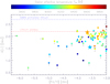 |
Fig. 9 Lithium abundance vs. metallicity [Fe/H] in CS 22876-032A and B (large stars), compared with the literature measurements (small circles) in unevolved stars with [Fe/H] < −3.0 and log g > 3.0. Downward arrows indicate upper limits. The blue dashed line is the predicted SBBN primordial lithium abundance and the red dash-dotted line is the value of the lithium plateau, known as the Spite Plateau. |
Acknowledgements
J.I.G.H. acknowledges financial support from the Spanish Ministry of Science, Innovation and Universities (MICIU) under the 2013 Ramón y Cajal program RYC-2013-14875, and also from the Spanish Ministry project MICIU AYA2017-86389-P. P.B. and E.C. acknowledge support from the Scientific Council of Observatoire de Paris and from the Programme National de Physique Stellaire of the Institut National des Sciences de l’Univers - CNRS. H.G.L. acknowledges financial support from the Sonderforschungsbereich SFB 881 “The Milky Way System” (subproject A4) of the German Research Foundation (DFG).
References
- Aguado, D. S., Allende Prieto, C., González Hernández, J. I., & Rebolo, R. 2018, ApJ, 854, L34 [NASA ADS] [CrossRef] [Google Scholar]
- Aguado, D. S., González Hernández, J. I., Allende Prieto, C., & Rebolo, R. 2019, ApJ, 874, L21 [NASA ADS] [CrossRef] [Google Scholar]
- Aoki, W., Barklem, P. S., Beers, T. C., et al. 2009, ApJ, 698, 1803 [NASA ADS] [CrossRef] [Google Scholar]
- Aoki, W., Ito, H., & Tajitsu, A. 2012, ApJ, 751, L6 [NASA ADS] [CrossRef] [Google Scholar]
- Asplund, M., Lambert, D. L., Nissen, P. E., Primas, F., & Smith, V. V. 2006, ApJ, 644, 229 [NASA ADS] [CrossRef] [Google Scholar]
- Boesgaard, A. M., Rich, J. A., Levesque, E. M., & Bowler, B. P. 2011, ApJ, 743, 140 [NASA ADS] [CrossRef] [Google Scholar]
- Bonifacio, P. 2005, Mem. Soc. Astron. It. Suppl., 8, 114 [Google Scholar]
- Bonifacio, P., & Molaro, P. 1997, MNRAS, 285, 847 [NASA ADS] [CrossRef] [Google Scholar]
- Bonifacio, P., Molaro, P., Sivarani, T., et al. 2007a, A&A, 462, 851 [NASA ADS] [CrossRef] [EDP Sciences] [Google Scholar]
- Bonifacio, P., Pasquini, L., Molaro, P., et al. 2007b, A&A, 470, 153 [NASA ADS] [CrossRef] [EDP Sciences] [Google Scholar]
- Bonifacio, P., Sbordone, L., Caffau, E., et al. 2012, A&A, 542, A87 [NASA ADS] [CrossRef] [EDP Sciences] [Google Scholar]
- Bonifacio, P., Caffau, E., Spite, M., et al. 2015, A&A, 579, A28 [NASA ADS] [CrossRef] [EDP Sciences] [Google Scholar]
- Bonifacio, P., Caffau, E., Spite, M., et al. 2018, A&A, 612, A65 [NASA ADS] [CrossRef] [EDP Sciences] [Google Scholar]
- Bonifacio, P., Caffau, E., Spite, M., & Spite, F. 2019, Res. Notes AAS, 3, 64 [Google Scholar]
- Caffau, E., Bonifacio, P., François, P., et al. 2011, Nature, 477, 67 [NASA ADS] [CrossRef] [PubMed] [Google Scholar]
- Cayrel, R., Spite, M., Spite, F., et al. 1999, A&A, 343, 923 [NASA ADS] [Google Scholar]
- Cayrel, R., Steffen, M., Chand, H., et al. 2007, A&A, 473, L37 [NASA ADS] [CrossRef] [EDP Sciences] [Google Scholar]
- Coc, A., & Vangioni, E. 2017, Int. J. Mod. Phys. E, 26, 1741002 [Google Scholar]
- Cyburt, R. H., Fields, B. D., Olive, K. A., & Yeh, T.-H. 2016, Rev. Mod. Phys., 88, 015004 [NASA ADS] [CrossRef] [Google Scholar]
- Fields, B. D., Molaro, P., & Sarkar, S. 2014, Chin. Phys. C, 38, 339 [Google Scholar]
- Frebel, A., Aoki, W., Christlieb, N., et al. 2005, Nature, 434, 871 [NASA ADS] [CrossRef] [PubMed] [Google Scholar]
- González Hernández, J. I., Bonifacio, P., Ludwig, H.-G., et al. 2008, A&A, 480, 233 [NASA ADS] [CrossRef] [EDP Sciences] [MathSciNet] [Google Scholar]
- González Hernández, J. I., Bonifacio, P., Caffau, E., et al. 2009, A&A, 505, L13 [NASA ADS] [CrossRef] [EDP Sciences] [Google Scholar]
- González Hernández, J. I., Pepe, F., Molaro, P., & Santos, N. C. 2018, Handbook of Exoplanets (Berlin: Springer), 157 [Google Scholar]
- Hansen, T., Hansen, C. J., Christlieb, N., et al. 2014, ApJ, 787, 162 [NASA ADS] [CrossRef] [Google Scholar]
- Hansen, T., Hansen, C. J., Christlieb, N., et al. 2015, ApJ, 807, 173 [NASA ADS] [CrossRef] [Google Scholar]
- Iglesias-Marzoa, R., López-Morales, M., & Jesús Arévalo Morales, M. 2015, PASP, 127, 567 [NASA ADS] [CrossRef] [Google Scholar]
- Ito, H., Aoki, W., Beers, T. C., et al. 2013, ApJ, 773, 33 [NASA ADS] [CrossRef] [Google Scholar]
- Jedamzik, K., & Pospelov, M. 2009, New J. Phys., 11, 105028 [NASA ADS] [CrossRef] [Google Scholar]
- Klevas, J., Kučinskas, A., Steffen, M., Caffau, E., & Ludwig, H. G. 2016, A&A, 586, A156 [NASA ADS] [CrossRef] [EDP Sciences] [Google Scholar]
- Lind, K., Melendez, J., Asplund, M., Collet, R., & Magic, Z. 2013, A&A, 554, A96 [NASA ADS] [CrossRef] [EDP Sciences] [Google Scholar]
- Ludwig, H.-G., Caffau, E., Steffen, M., et al. 2009, Mem. Soc. Astron. It., 80, 711 [NASA ADS] [Google Scholar]
- Markwardt, C. B. 2009, in Astronomical Data, Analysis Software and Systems XVIII, eds. D. A. Bohlender, D. Durand, & P. Dowler, ASP Conf. Ser., 411, 251 [Google Scholar]
- Matsuno, T., Aoki, W., Suda, T., & Li, H. 2017, PASJ, 69, 24 [NASA ADS] [CrossRef] [Google Scholar]
- Meléndez, J., Ramírez, I., Casagrande, L., et al. 2010, Ap&SS, 328, 193 [NASA ADS] [CrossRef] [Google Scholar]
- Molaro, P., & Castelli, F. 1990, A&A, 228, 426 [NASA ADS] [Google Scholar]
- Mott, A., Steffen, M., Caffau, E., Spada, F., & Strassmeier, K. G. 2017, A&A, 604, A44 [NASA ADS] [CrossRef] [EDP Sciences] [Google Scholar]
- Norris, J. E., Beers, T. C., & Ryan, S. G. 2000, ApJ, 540, 456 [NASA ADS] [CrossRef] [Google Scholar]
- Pepe, F., Molaro, P., Cristiani, S., et al. 2014, Astron. Nachr., 335, 8 [NASA ADS] [CrossRef] [Google Scholar]
- Planck Collaboration XIII. 2016, A&A, 594, A13 [NASA ADS] [CrossRef] [EDP Sciences] [Google Scholar]
- Prantzos, N. 2012, A&A, 542, A67 [NASA ADS] [CrossRef] [EDP Sciences] [Google Scholar]
- Rebolo, R., Molaro, P., & Beckman, J. E. 1988, A&A, 192, 192 [NASA ADS] [Google Scholar]
- Rollinde, E., Vangioni, E., & Olive, K. A. 2006, ApJ, 651, 658 [NASA ADS] [CrossRef] [Google Scholar]
- Ryan, S. G., Beers, T. C., Kajino, T., & Rosolankova, K. 2001, ApJ, 547, 231 [NASA ADS] [CrossRef] [Google Scholar]
- Sbordone, L., Bonifacio, P., Caffau, E., et al. 2010, A&A, 522, A26 [NASA ADS] [CrossRef] [EDP Sciences] [Google Scholar]
- Spergel, D. N., Bean, R., Doré, O., et al. 2007, ApJS, 170, 377 [NASA ADS] [CrossRef] [Google Scholar]
- Spite, M., & Spite, F. 1982, Nature, 297, 483 [NASA ADS] [CrossRef] [Google Scholar]
- Spite, M., Bonifacio, P., Spite, F., et al. 2019, A&A, 624, A44 [NASA ADS] [CrossRef] [EDP Sciences] [Google Scholar]
- Starkenburg, E., Aguado, D. S., Bonifacio, P., et al. 2018, MNRAS, 481, 3838 [NASA ADS] [CrossRef] [Google Scholar]
- Steffen, M., Cayrel, R., Caffau, E., et al. 2012, Mem. Soc. Astron. It. Suppl., 22, 152 [Google Scholar]
- Steffen, M., Prakapavičius, D., Caffau, E., et al. 2015, A&A, 583, A57 [NASA ADS] [CrossRef] [EDP Sciences] [Google Scholar]
- Steigman, G. 2007, Ann. Rev. Nucl. Part. Sci., 57, 463 [Google Scholar]
All Tables
All Figures
|
Fig. 1 Radial velocities of the primary (star A: filled symbols) and the secondary (star B: open symbols) of CS 22876–032 (upper panel), and residuals from the fit (lower panel). Triangles and circles are literature (Norris et al. 2000; González Hernández et al. 2008) and new UVES observations, respectively. The curves show the orbital solution (see Table 1) for star A (solid) and B (dashed). Triple dotted-dashed horizontal line shows the centre-of-mass velocity of the system. |
| In the text | |
|
Fig. 2 Normalised, co-added, RV-corrected, unveiled spectrum of CS 22876–032 shown in the spectral region of the Mg Ib triplet (upper panel) and rebinned to a wavelength step of 0.014 Å pixel−1 (lower panel) in the rest frame of star A. |
| In the text | |
|
Fig. 3 Normalised, co-added, RV-corrected, unveiled spectrum of CS 22876–032A (blue dots), together with best-fit 3D-NLTE Li profile (red circles), and residuals of the fit (lower panel). The mean flux uncertainty is shown on the right as a blue circle with error bars. The horizontal dashed and dot-dashed lines indicate the 1σ dispersion of the observed flux points relative to the mean difference observed minus computed profiles. |
| In the text | |
|
Fig. 4 Density distributions of lithium isotopic ratio vs. broadening velocity of 10 000 Monte Carlo simulations to evaluatethe confidence of the best fit to the Li profile of star A. The green dash-dotted lines indicate the 1σ uncertainty,whereas the blue dotted and red dashed lines are the best fit values and the centre of the distributions, respectively. |
| In the text | |
|
Fig. 5 Same as Fig. 4, but for the lithium isotopic ratio vs. lithium abundance. About 70% of the simulations shown here fall at vBR ≥ 0 and 6 Li/7Li ≥ 0. |
| In the text | |
|
Fig. 6 Best fit (red circles) to the unveiled Li profile of star A (blue circles) rebinned to a wavelength step of 0.014 Å pixel−1 (upper panel) and the residuals of the fit (lower panel). |
| In the text | |
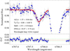 |
Fig. 7 Same as Fig. 6, but for star B. |
| In the text | |
|
Fig. 8 Lithium abundance vs. effective temperature in CS 22876-032A and B (large stars), compared with the literature measurements (small circles) in unevolved stars with [Fe/H] < −3.0 and log g > 3.0. Downward arrows indicate upper limits. The histogram on the right side shows the Li measurements without including the upper-limit values. The blue dashed line is the predicted SBBN primordial lithium abundance and the red dash-dotted line is the value of the lithium plateau, known as the Spite Plateau. |
| In the text | |
|
Fig. 9 Lithium abundance vs. metallicity [Fe/H] in CS 22876-032A and B (large stars), compared with the literature measurements (small circles) in unevolved stars with [Fe/H] < −3.0 and log g > 3.0. Downward arrows indicate upper limits. The blue dashed line is the predicted SBBN primordial lithium abundance and the red dash-dotted line is the value of the lithium plateau, known as the Spite Plateau. |
| In the text | |
Current usage metrics show cumulative count of Article Views (full-text article views including HTML views, PDF and ePub downloads, according to the available data) and Abstracts Views on Vision4Press platform.
Data correspond to usage on the plateform after 2015. The current usage metrics is available 48-96 hours after online publication and is updated daily on week days.
Initial download of the metrics may take a while.