| Issue |
A&A
Volume 626, June 2019
|
|
|---|---|---|
| Article Number | A4 | |
| Number of page(s) | 16 | |
| Section | The Sun | |
| DOI | https://doi.org/10.1051/0004-6361/201834811 | |
| Published online | 30 May 2019 | |
Automating Ellerman bomb detection in ultraviolet continua
1
Institute for Solar Physics, Department of Astronomy, Stockholm University, AlbaNova University Centre, 106 91 Stockholm, Sweden
e-mail: gregal.vissers@astro.su.se
2
Institute of Theoretical Astrophysics, University of Oslo, PO Box 1029 Blindern, 0315 Oslo, Norway
3
Rosseland Centre for Solar Physics, University of Oslo, PO Box 1029 Blindern, 0315 Oslo, Norway
4
Lingezicht Astrophysics, ’t Oosteneind 9, 4158 CA Deil, The Netherlands
Received:
10
December
2018
Accepted:
23
January
2019
Ellerman bombs are transient brightenings in the wings of Hα 6563 Å that pinpoint photospheric sites of magnetic reconnection in solar active regions. Their partial visibility in the 1600 Å and 1700 Å continua registered routinely by the Atmospheric Imaging Assembly (AIA) onboard the Solar Dynamics Observatory (SDO) offers a unique opportunity to inventory such magnetic-field disruptions throughout the AIA database if a reliable recipe for their detection can be formulated. This is done here. We have improved and applied an Hα Ellerman bomb detection code to ten data sets spanning viewing angles from solar disc centre to the limb. They combine high-quality Hα imaging spectroscopy from the Swedish 1 m Solar Telescope with simultaneous AIA imaging around 1600 Å and 1700 Å. A trial grid of brightness, lifetime and area constraints is imposed on the AIA images to define optimal recovery of the 1735 Ellerman bombs detected in Hα. The best results when optimising simultaneously for recovery fraction and reliability are obtained from 1700 Å images by requiring 5σ brightening above the average 1700 Å nearby quiet-Sun intensity, lifetime above one minute, area of 1–18 AIA pixels. With this recipe 27% of the AIA detections are Hα-detected Ellerman bombs while it recovers 19% of these (of which many are smaller than the AIA resolution). Better yet, among the top 10% AIA 1700 Å detections selected with combined brightness, lifetime and area thresholds as many as 80% are Hα Ellerman bombs. Automated selection of the best 1700 Å candidates therefore opens the entire AIA database for detecting most of the more significant photospheric reconnection events. This proxy is applicable as a flux-dynamics tell-tale in studying any Earth-side solar active region since early 2010 up to the present.
Key words: Sun: activity / Sun: atmosphere / Sun: magnetic fields / Sun: UV radiation
© ESO 2019
1. Introduction
Ellerman bombs (Ellerman 1917) are among the most spectacular small-scale eruptive events in the solar spectrum. In the outer wings of Hα 6563 Å they display flame morphology with highly dynamic sub-structuring at the resolution limit of current high-resolution telescopes (e.g. Hashimoto et al. 2010; Watanabe et al. 2011; Nelson et al. 2015; Rouppe van der Voort et al. 2017). They are predominantly observed near polarity inversion lines (e.g. Georgoulis et al. 2002; Fang et al. 2006; Pariat et al. 2007; Matsumoto et al. 2008; Hashimoto et al. 2010; Vissers et al. 2013; Reid et al. 2016) in regions where magnetic field patterns on the solar surface change much, such as emerging flux regions and rapidly emerging or decaying active regions. They pinpoint reconnection in the solar photosphere.
The numerical simulations of Archontis & Hood (2009) already suggested that Ellerman bombs represent a flux-emergence phenomenon. More advanced numerical simulations including Hα 6563 Å synthesis have recently confirmed that small-scale magnetic reconnection within the photosphere is indeed their driving agent. Hansteen et al. (2017) did so for stronger-field events with the Bifrost code; Danilovic (2017) for weaker-field events with the MURaM code. The latter resemble the quiet-Sun Ellerman-like brightenings (QSEB) discovered by Rouppe van der Voort et al. (2016).
Ellerman bombs are classically identified through their large Hα 6563 Å wing brightening, but they can also be seen as wing enhancements in other chromospheric lines including Ca II H at 3968 Å (Matsumoto et al. 2008; Hashimoto et al. 2010; Rezaei & Beck 2015), Ca II 8542 Å (Fang et al. 2006; Socas-Navarro et al. 2006; Pariat et al. 2007; Reardon et al. 2013; Vissers et al. 2013), He I D3 at 5876 Å and He I 10830 Å (Libbrecht et al. 2017), and in the ultraviolet sampled by the Interface Region Imaging Spectrograph (IRIS; De Pontieu et al. 2014) as enhancements of the Mg II, C II and Si IV resonance lines (Vissers et al. 2015a; Grubecka et al. 2016). Of these the Si IV lines near 1400 Å are most informative because Ellerman bombs can appear optically thin in these and display bimodal-jet structure directly (Vissers et al. 2015a).
Ellerman bombs are generally also observed as brightenings in the 1600 Å and 1700 Å continua that normally originate from the upper photosphere (e.g. Qiu et al. 2000; Georgoulis et al. 2002; Pariat et al. 2007; Berlicki et al. 2010; Herlender & Berlicki 2011; Vissers et al. 2013; Rutten et al. 2013; Rezaei & Beck 2015; Chen et al. 2017). However, they have not been detected in the Na I D and Mg I b lines (Ellerman 1917; Rutten et al. 2015) formed at similar heights. This apparent contradiction was attributed by Rutten (2016) to ionisation of the neutral metal stages combined with non-equilibrium over-opacity in the scattering Balmer continuum, but this issue has not yet been addressed with numerical modelling. Non-equilibrium simulation and spectral synthesis are likely required to explain it, but even without understanding the brightness signatures of Ellerman bombs in mid-ultraviolet continua we may yet exploit them for Ellerman bomb detection and localisation.
The launch of the Solar Dynamics Observatory (SDO) in February 2010 has resulted in continuous monitoring of the whole Earth-facing side of the Sun ever since (and hopefully for years to come) in nine ultraviolet passbands including wide ones around 1600 Å and around 1700 Å with the Atmospheric Imaging Assembly (AIA). SDO also collects photospheric magnetograms with the Helioseismic and Magnetic Imager (HMI), but recognising small-scale reconnection events from photospheric flux cancelations requires higher angular resolution and magnetic sensitivity than what HMI provides. While deep learning techniques may improve this shortcoming (Díaz Baso & Asensio Ramos 2018), Ellerman bombs already present a viable alternative to locate photospheric reconnection events, not by displaying the bipolar input prior to cancelation but by displaying the resulting energy output.
Thus, the occurrence of Ellerman bombs may be used to detect and trace small-scale solar magnetic field reorganisation, making them an effective proxy for (on-going) flux emergence and an early warning of solar activity. This makes it desirable to be able to pinpoint Ellerman bombs anywhere at any time, not only from highest-quality Hα observing as done so far. The latter requires the very best seeing at the very best telescopes and is therefore severely limited to rare observation, short sampling duration, and small field of view so that most Ellerman bomb studies have analysed only one or only a few. Characterising Ellerman bomb signatures in mid-ultraviolet images and defining a reliable detection recipe that only requires the ubiquitous AIA data (over 10 million 1600–1700 Å full-disc image pairs to date) is obviously a worthwhile quest. We have undertaken that quest here. A similar Hα–AIA 1700 Å correspondence study was recently done by Chen et al. (2017) but only for a single observation; here, we cover the full centre-limb variation and a variety of active regions by analysing ten different data sets.
Reliable identification of Ellerman bombs is non-trivial both in the Hα wings and in the ultraviolet continua due to competing small-scale brightness features of differing nature. At low brightness these are the magnetic concentrations that constitute network and plage and were described as “magnetic bright points” and modelled as magnetostatic fluxtubes in the older literature. Their observation requires sub-arcsecond resolution to avoid cancelation of their brightness against the darkness of the intergranular lanes in which they reside (Title & Berger 1996) and only with the superior resolution of the Swedish 1 m Solar Telescope (SST; Scharmer et al. 2003a) they were resolved into intricate morphologies (Berger et al. 2004). These concentrations also show enhanced brightening in the Hα wings (Leenaarts et al. 2006a,b), due to deeper fluxtube hole visibility through reduced collisional damping at lower density. We call these ubiquitous brightenings “pseudo-EBs” following Rutten et al. (2013) who note that a significant fraction of the Ellerman bomb literature mistakenly addressed them, although Ellerman (1917) already warned against facular confusion.
The non-reconnecting magnetic concentrations also appear bright in ultraviolet continua, probably from larger fluxtube transparency by ionisation of Si I, Mg I, Fe I and Al I, so that lower-brightness selection thresholds must be used not only for Hα but also for the 1600 and 1700 Å images. The 1600 Å images display Ellerman bombs at higher contrast over the quiescent network than the 1700 Å images, and also larger (Fig. 2 below). These enhancements are likely due to extra emission and scattering in the C IV resonance lines in the 1600 Å passband.
At high brightness the major cause of misidentification are the flaring active-region fibrils (FAF) described in Vissers et al. (2015a) and Rutten (2016) and possibly named microflares elsewhere. They appear primarily in the 1600 Å images, probably due to large C IV contribution; in the 1700 Å images they are much weaker or absent. In 1600 Å movies one recognises them by their sudden appearance, large brightness, extended elongated shape, and very fast apparent motion along filamentary tracks. They, or their aftermaths, show large emission in the IRIS lines and also leave signatures in the AIA EUV passbands (Vissers et al. 2015a), whereas Ellerman bombs may show up in the IRIS lines too but weaker and do not affect the overlying fibrils observed in the core of Hα (as already remarked by Ellerman 1917) and similarly in the cores of Mg II h and k.
More generally sudden, small, energetic brightenings observed in the ultraviolet are called UV bursts. They are reviewed comprehensively in Young et al. (2018) and include the IRIS bursts of Peter et al. (2014), FAFs, and also part of the Hα-identified Ellerman bomb population but without complete overlap (Vissers et al. 2015a; Kim et al. 2015; Tian et al. 2016; Libbrecht et al. 2017). This partial non-correspondence seems primarily due to difference in height of the energy-releasing reconnection event. Observationally this is suggested by common UV-burst response in chromospheric and transition-region diagnostics whereas Ellerman bombs show no counterpart in the hotter AIA channels. Computationally it is suggested by the simulation results of Hansteen et al. (2017) who reproduce Ellerman bombs from lower-height reconnection and UV bursts from larger-height reconnection, but this simulation did not produce both signatures simultaneously whereas the observed populations do overlap.
The observational mix of small-feature brightenings in the form of pseudo-EBs, bona fide Ellerman bombs, FAFs, and other UV bursts make unequivocal Ellerman bomb identification a difficult task. Over the past years we have gained considerable experience in recognising them in the many pertinent Hα data sets which the Oslo group collected at the SST, employing the versatile CRISPEX browser (Vissers & Rouppe van der Voort 2012; Löfdahl et al. 2018) for interactive inspection. A major Hα tell-tale is flame morphology in limbward viewing, first demonstrated in Watanabe et al. (2011) and also the key diagnostic in recognising QSEBs (Rouppe van der Voort et al. 2016). Others are the sudden Ellerman bomb appearance and their rapid fine-structure variation. Together, these give us confidence in separating Ellerman bombs from network pseudo-EBs in high quality SST data. In 1600 Å images smallness, roundish non-filamentary shape, and larger stationarity distinguish Ellerman bombs from FAFs.
Our expertise in Ellerman bomb identification in SST data relies critically on the superior resolution obtained with this superb telescope. In contrast, AIA’s resolution is ten times worse; we show below that most SST Hα Ellerman bombs are smaller than a single AIA pixel. This suggests that recovering Hα Ellerman bombs in AIA images is hampered severely by lack of resolution, but it should be noted that whereas Ellerman bombs have optically thin formation of their outer Hα wing brightenings, permitting scattering-free intensity variations over very fine scales (“striations”) as indeed observed (Watanabe et al. 2011), the ultraviolet continua are strongly scattering which results in apparent feature spreading and smoothing over a few hundred km (Fig. 36 of Vernazza et al. 1981). Also, the steeper Planck function sensitivity at shorter wavelengths enhances ultraviolet contrasts. Thus, very fine sub-pixel intensity spikes can still cause full-AIA-pixel brightening.
In summary, we aim here to establish the combination of feature parameter values (brightness, lifetime, area, etc.) applicable to mid-ultraviolet AIA images that provides optimal recovery of Hα-detected Ellerman bombs. The remainder of this publication is structured as follows. The observations and data reduction are described in Sect. 2, the analysis method in Sect. 3. In Sect. 4 we present the results followed by discussion (Sect. 5) and conclusions (Sect. 6). The latter end with recommendations for Ellerman bomb-detection in the AIA database which represent our “take-away” message.
2. Observations and data reduction
2.1. SST data acquisition and reduction
In this study we used ten data sets from the CRisp Imaging Spectropolarimeter (CRISP; Scharmer et al. 2008) at the SST for which AIA 1600 Å and 1700 Å data are also available. They are detailed in Table 1. Their outstanding quality benefited much from the SST’s adaptive-optics wave-front correction system (Scharmer et al. 2003b) and from further image reconstruction using Multi-Object Multi-Frame Blind Deconvolution (MOMFBD; van Noort et al. 2005). Data sets C, D and F were reduced using the CRISPRED processing pipeline of (de la Cruz Rodríguez et al. 2015) while the remainder was processed using a predecessor of this framework.
Overview over the data sets analysed in this study.
The Hα 6563 Å line was typically observed with wavelength scans out to ±1.5–2.1 Å, with fixed wavelength spacing for half of the data sets, while the other half had denser sampling in the core but sparser sampling in the outer wings (cf. the eighth (Range) and ninth (Δλ) columns in Table 1 for further details). All but the last data sets were complemented with Ca II 8542 Å observations. Sets A, C–G and I also included full Stokes polarimetry in Fe I 6301.4 Å (sampling only one wing position at −0.048 Å except for set C where the line was scanned out to ±0.6 Å). However, in this study we use only the Hα data.
All observations targeted active regions in various stages of their evolution; their numbers are specified in the third column of Table 1. In his discovery paper Ellerman (1917) described his bombs (he called them hydrogen bombs) as exclusively occurring near sunspots in emerging complex active regions, but they are also seen near actively flux-shredding sunspots in strongly decaying active regions with similar serpentine field bundles as in emerging-flux regions, also producing moving magnetic features (Harvey & Harvey 1973). The Ellerman bombs in data sets A, B and E–I can be generally considered as moat flow events, with moat flow defined as an organised streaming motion near a sunspot. Those in F, G and I were around sunspots in generally decaying active regions, while those in sets C, D and J occurred in–or as part of–(recently) emerging flux.
In addition, we note that data sets A, E and H cover (in reverse order) the same sunspot while it rotated over the disc displaying stable levels of average activity throughout (no reported flares), set C was obtained in a highly complex active region with on-going flux emergence (here observed only two days after it received its NOAA AR number, a time in which its total sunspot area grew by over 420% and it produced one M-class and nine C-class flares), set D covered the trailing part of an active region while in the leading part an M-class flare went off towards the end of our observation, and set I targeted an active region that, while decaying, was still relatively complex containing three sunspots. Finally, set E was previously analysed by Vissers et al. (2013), set F by Vissers et al. (2015b) in studying penumbral microjets, and set J by Rouppe van der Voort et al. (2016) in studying QSEBs far away from the active region. In addition, SST/CRISP observations of active region NOAA AR 11504 (data set I) from one day later were analysed in Nelson et al. (2015) and Reid et al. (2015).
2.2. SDO data collection and co-alignment
Corresponding SDO image cutout sequences for the ten SST/CRISP data sets were downloaded, precisely cross-aligned (all AIA channels to HMI), and co-aligned with the SST images using an IDL pipeline developed by the third author. It is available at his website1 and will be detailed elsewhere. For each SST data set its product consists of eleven HMI and AIA image cutout sequences that are rotated to the SST image orientation and resampled to be precisely co-spatial (to within  ) and as close as possible in time (through nearest-neighbour frame selection) with the SST images. The SDO data were interpolated to the ten times finer SST pixel scale using nearest-neighbour sampling to maintain the original AIA pixel shapes for determining area constraints on their native scale. The AIA EUV sequences are not used in this analysis, only the mid-ultraviolet (1600 Å and 1700 Å) and HMI ones.
Figure 1 shows co-aligned sample images in CRISP Hα and AIA 1700 Å from all ten data sets. Generally, there is good spatial correspondence between the brightest features in each pair, but there are also many differences. Figure 2 shows sample comparisons of AIA 1600 and 1700 Å image cutouts for four data sets at the same sample times as in Fig. 1 to illustrate differences between these AIA diagnostics. In this figure each panel is not byte-scaled individually with its own saturation clip as done for best scene visibility in Fig. 1, but each pair shows the square root of the intensity at a common range set by requiring that the quiet-area averages defined by the masks defined below (taken over the whole time sequence) obtain the same apparent brightness, with the same high-level saturation cutoff per pair and without clipping the 1700 Å images.
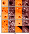 |
Fig. 1. Full field-of-view samples of all 10 data sets. Panel pairs (A)–(J) show near-simultaneous co-aligned CRISP Hα-wing images (orange; blue-wing images averaged around −1 Å for all but data set B that shows the red wing at +1 Å) and AIA 1700 Å images (red-brown), ordered by decreasing viewing angle μ (= cos θ, with θ the angle between the line-of-sight and the normal to the solar surface) specified at lower-left in each AIA panel with the image-centre solar (X, Y) location. The times of the SST observations are specified at lower-left in each CRISP panel. The corresponding AIA image cutouts were interpolated to these from their 24 s sampling cadence (through nearest-neighbour frame selection) and rotated to the SST orientation. Each field of view has been cut slightly to obtain the same display size and scale. The arrows at top left in each AIA panel point towards solar north (red), west (blue) and the nearest limb (white). Each image is byte-scaled independently including high-level clipping to improve the overall scene visibility. Dashed frames in pairs C, D, F and I define cutouts for Fig. 2, solid frames in pair E define cutouts for Fig. 4. |
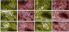 |
Fig. 2. Feature visibilities in AIA 1600 Å (first and third columns) and 1700 Å (second and fourth columns). The panel pairs show selected cutouts for data sets A, C, D, F, H and I, labelled with their μ values in the 1600 Å panels. The cutout locations are outlined by dashed frames in the corresponding panels of Fig. 1. In order to accommodate the dynamic range the square root of the intensity is shown. The byte scaling is common between pairs and is defined so that quiet areas obtain the same apparent average brightness in 1600 and 1700 Å at a scale that saturates at 15σ above this quiet average for 1700 Å except for set F where 10σ was used to for better display contrast. At these values no 1700 Å image is clipped; only the brightest 1600 Å features are. The blue contours outline 1700 Å areas at least 5σ above the quiet average. Major tick marks are spaced 10″ apart, minor tick marks 2″ as in Fig. 1. |
The quiet parts appear very similar between 1600 and 1700 Å, showing nearly identical bright-grain patterns. The internetwork hearts between these appear darker in 1600 Å which is probably due to longer exposure (about 3 s instead of 1 s) that causes more smearing of the rapidly moving filamentary weak-brightness patterns set by interfering acoustic shocks.
The scaling also makes clear that both Ellerman bombs (bright and roundish in both) and FAFs (elongated bright features in 1600 Å not present in 1700 Å) reach higher contrast over the quiescent network in 1600 Å, presumably from C IV contributions. They also appear slightly larger, presumably from scattering. The common 5σ above-quiet-average 1700 Å brightness contours in Fig. 2 illustrate one ingredient of the Ellerman bomb detection recipe developed below.
3. Analysis methods
3.1. Automated detection with EBDETECT
Our aim is to establish the optimal recipe to retrieve Hα-detected Ellerman bombs from concurrent AIA ultraviolet images. We therefore first detect Ellerman bombs in the CRISP Hα data and then use these to evaluate the recovery success of various AIA detection criteria including finding which AIA passband works best.
Our detection code EBDETECT2 (written in IDL) used for both the SST and the AIA data builds on four key elements:
– Brightness thresholds. Initial identification is done by selecting pixels passing a specified intensity threshold. For Hα a double intensity-threshold criterion (on wing-average images as defined further down) serves to recognise both the high-intensity fine-structure kernel and the surrounding lower intensity halo. These thresholds are expressed in the average intensity and the standard deviation around that for all pixels in quiet areas of the field of view over the full sequence duration as defined below.
– Size constraints. A minimum area is set to prevent selecting single-pixel features that are likely spurious signals, while setting a maximum prevents picking up extended regions of plage (a particular issue for the AIA images at low brightness threshold).
– Continuity constraints. Detections are subsequently checked for overlap between sequential frames, requiring at least one pixel area (native size, i.e. 0.6″ × 0.6″ for AIA, 0.059″ × 0.059″ for SST) overlap from frame to frame. However, in order to alleviate bad seeing moments there may be intermediate gaps of durations up to the minimum-lifetime constraint (i.e. up to ∼60 s).
– Lifetime constraint. Finally, those detections that have passed the above hurdles must also live longer than 1 min.
EBDETECT builds on criteria established in Watanabe et al. (2011). Earlier versions were used in Vissers et al. (2013), also for detection in Ca II 8542 Å, and Vissers et al. (2015a) while Vissers et al. (2019) employ the current version. The key changes from our earlier versions are firstly, the values of the brightness thresholds and how these are determined, and secondly for Hα thresholds are now applied to the blue and red wings. We first detail these changes.
3.1.1. Reference intensities for brightness thresholding
The first modification serves to define dataset-independent brightness thresholds. In our previous Hα studies a double brightness threshold of 155% and 140% of the average brightness generally yielded good results, but this average was evaluated over the full fields of view. This had to be amended for cases where the umbral and/or penumbral areas were relatively small by varying the two thresholds over 160–145% and 145–130%, respectively. Such target- and reference-dependent variations are not uncommon, as shown by Table 2 which lists thresholds used during the past 40 years, but they hinder the definition of a general recipe. We therefore now define thresholds no longer with respect to the average over the full field of view, but only over its quiet areas, i.e. excluding sunspots, pores and significantly bright plage. In several studies the Hα wing enhancement was normalised by nearby quiet-area averages, but here we average over all quiet pixels in each field of view to obtain better statistics. This approach requires automated definition of blocking masks.
Hα intensity, area and lifetime thresholds for Ellerman bomb selection and resulting detection rates in recent literature.
A straightforward approach would seem to mask out the stronger-field magnetic areas on co-aligned HMI line-of-sight magnetograms, but substantial offsets between HMI magnetogram contours and HMI continuum-image contours can occur away from disc centre. We therefore define a composite mask by first thresholding the HMI continuum images at 60% of their maximum intensity to discard darker sunspots and pores, and then combine this low-intensity block with magnetogram blocking above |Blos| = μ × 180 Gauss which also removes bright plage. Such masks are determined for every image and then multiplicatively compounded into a single composite mask used for the full sequence so that a pixel blocked at any time gets blocked at all times. Any passed feature smaller than 4 AIA pixel-equivalent area (about 400 SST pixels) is then also blocked, as are those smaller than 60 AIA pixel-equivalent area if they lie isolated within a blocked region (e.g. a bright penumbral feature). Figure 3 shows results from this procedure.
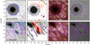 |
Fig. 3. HMI mask construction for data sets A (viewing angle μ = 0.93, top row) and I (μ = 0.36, bottom row). The masks serve to define the local quiet area for reference brightness thresholding. Left to right: HMI continuum image, HMI line-of-sight magnetogram (positive polarity in red, negative in black, zero field strength white), AIA 1700 Å image, blue wing Hα image. The HMI intensity mask is outlined by blue contours in the first column, the HMI magnetic field mask by green contours in the second column. The composite mask is shown in all panels by purple dashed contours. The small green-only islands in the second column are blocked by the minimum-area constraint. In the last panel the blocked part covers most of the upper half including all Ellerman bombs. |
For data set J, which contains the limb in the field of view, we applied an additional limb mask blocking the off-limb pixels and also the outer ∼5″ of the disc because its large radial intensity drop strongly influences the mean value.
3.1.2. Hα wing treatment
The second modification addresses extreme Doppler shifts of Hα that are imposed by fast flows in overlying canopy fibrils. In previous studies we used wing-average images constructed as Iw ≡ (Ib + Ir)/2, where the blue-wing Ib and red-wing Ir are the spectral averages over three wavelength tuning positions centred at −1 Å and +1 Å, respectively (i.e. effectively ±(0.9–1.1) Å). However, in the presence of strong canopy Doppler shifts using such mean value combining both wings can put the intensity below the threshold and so reduce the apparent area of Ellerman bomb candidates or ignore them altogether. To account for these effects we therefore apply the brightness thresholding to the wing-averages Ib and Ir separately, i.e. a pixel need only pass the threshold in one of the wings to still carry over to the next step (an approach similar to the one in Reid et al. 2016, except that they also included a line core constraint). In the remainder we refer to Ib and Ir as wing-average images. Due to larger spacing of the wavelength sampling in datasets C, D and F, for those cases this averaging effectively spans ±(0.8–1.2) Å.
3.2. Parameter values for Ellerman bomb detection in Hα
For our Ellerman bomb detections in Hα wing-average images we ended up with the following constraints: (1) a double brightness threshold of 145% (core) and 130% (halo) over the quiet-Sun average which must be exceeded in at least one of the wings, where halo pixels are adjacent to already defined core or halo pixels, (2) a minimum area of 10 connected core-plus-halo SST pixels (corresponding to a linear extent of  depending on feature elongation, about 0.035 arcsec2), and (3) a minimum lifetime of about 60 s but allowing non-detection gaps up to about 60 s to accommodate bad-seeing instances. The latter time constraints translate into 2–7 frames depending on the observing cadence and effectively span 53–68 s.
Two further adjustments were made to account for particular data-set peculiarities. Firstly, in set A we found that the average intensities varied strongly in time, by nearly 12% between the first and last frames as compared to 0–4% for the other data sets. We compensated for this variation by taking a running mean with a boxcar of about 5 min (equivalent to 13 frames, spanning times over which the mean intensities changed less than 1%). This correction resulted in detecting events that were missed previously, especially in the beginning of the time sequence.
Secondly, the wing-average images of data sets I and J, which are the most limbward ones, were more strongly affected in the Hα wings at ±(0.9–1.1) Å by Dopplershifts of overlying canopy fibrils, which we remedied by moving the sampling wavelengths for the average taking outward to ±(1.0–1.2) Å. This correction resulted in fewer dubious small-scale weak detections.
Our Hα constraints resulted in the detection of 1735 candidates in total from our ten SST data sets. We verified their nature by visual inspection of the resulting Ellerman bomb contours overlaid on Hα wing-average images using CRISPEX and concluded that, even though there is a comparatively large population of very small-scale, short-lived events in data sets C, D, F and J for which identification is less obvious, at least 90% of the 1735 automated Hα detections represented bona fide Ellerman bombs. We also found that our recipe recovers over 94% of what we recognise as bona fide Ellerman bombs.
3.3. Parameter grid for Ellerman bomb detection with AIA
We applied EBDETECT to the AIA 1600 and 1700 Å sequences for a grid of parameter values that were varied independently. Firstly, eight brightness thresholds were considered, varying at 1σ steps between 3σ and 10σ above the average quiet-Sun intensity and its standard deviation σ determined using the same HMI-based masks as for Hα. Initial tests with thresholds at only 1σ and 2σ mis-identified too much normal network for any combination of the other parameters (as expected from the Hα-1700 Å scatter plots in Fig. 7 of Vissers et al. 2013), so we restricted the range to values from 3σ upwards.
Secondly, nine different area constraints were applied: a minimum of 1 AIA pixel-equivalent with a 3, 6, 9, ..., 24 and 27 AIA-pixel maximum. Since the AIA data were rescaled to the CRISP pixel size (while retaining the AIA pixel shapes, i.e. without interpolation) one AIA pixel corresponds to roughly 100–110 CRISP pixels; to be sure to catch single AIA pixels we lowered this value to 95 CRISP pixels as AIA pixel-equivalent for the lower limit while assuming 110 CRISP pixels as AIA single-pixel-equivalent for the upper limit.
Lastly, six different lifetime constraints were set: a 1 min minimum with a maximum of 5, 10, 15, 20, 30 min, or no maximum, respectively. The continuity criteria for the Hα detections were maintained: at least one native pixel overlap between frames while permitting up to about 1 min of non-detection (the latter only for consistency with the Hα formalism since AIA does not suffer seeing variations).
3.4. Correspondence evaluation using performance metrics
The next step is to compare the results of the AIA detection grid to the Ellerman bomb detections in Hα where we assume the latter to be all correct and also complete, i.e. that no Ellerman bombs went undetected. Of course, any automated detection code searching specific features must miss some and misidentify others, but we discard such errors for Hα on the basis of our visual checks.
For each AIA detection we then established whether there is overlap in time and space with any or multiple Hα detections, requiring overlaps during at least half the lifetime and half the area of one of the two detections. Tests where these requirements were varied down to only one third overlap and up to three quarters overlap in area and lifetime suggested no significant differences. Thus, for each AIA detection we so found whether it was correct (and if so, with how many Hα detections it overlapped) and added to the true positive (TP) AIA score or instead to the erroneous false positive (FP, without Hα counterpart) AIA score. The false negative (FN) score then remains as counting SST Hα detections without AIA counterpart. Table 3 visualises these in a contingency matrix, while Fig. 4 shows examples of valid TP detections and FP and FN error cases.
Contingencies for detection correspondence in Hα and AIA.
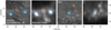 |
Fig. 4. Examples of detection evaluations from data set E. The two panel pairs show Hα−(0.9–1.1) Å blue-wing average intensity and AIA 1700 Å intensity for the similarly numbered cutouts in panel pair E of Fig. 1. Detection contours in Hα (cyan and orange) and AIA 1700 Å (blue and red; 5σ threshold, minimum of 1 AIA px and 2 frames visibility) are overlaid. The blue AIA contours (all panels) are classified as true positive (TP) detections from their degree of overlap with the cyan Hα contours (first and third panel), whereas the red contour in the first panel pair shows a false positive (FP), the orange contours in the second panel pair two false negatives (FN). |
To measure the success of a particular parameter combination we use the precision P defined as the fraction of Hα detections in all AIA detections
and the recall R defined as AIA’s recovery fraction of all Hα detections
A metric combining these is their equally-weighted harmonic mean:
which peaks where P and R are both high.
A crucial decision is what type of optimisation is desired. If one wishes to recover as many Ellerman bombs in AIA data as possible one should maximise the recall fraction R at the expense of the precision P, but if one instead desires that as many as possible of the AIA-detected events are Hα-verified Ellerman bombs the precision P should be maximised at the expense of the recall R. The F1 score covers the middle ground by maximising TP while minimising FP and FN. The priority choice between these three should be defined by the nature of the particular application. Here we present all three but focus on P and F1 because optimising R is not realistic at the tenfold SST–AIA resolution difference.
4. Results
4.1. Hα results
The Hα results are summarised in Table 4 and in Figs. 5 and 6. The detection rates (last column of Table 4) vary between 0.34–3.00 detections arcmin−1 min−1, similar to most studies over the past decade (cf. last column of Table 2). There is no obvious trend with viewing angle; all fall within 1σ spread from the average except for set C.
Hα detection statistics.
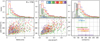 |
Fig. 5. Statistics of all 1735 Ellerman bomb detections in Hα. In all panels the ten different data sets are colour-coded blue-green-red-orange-purple along increasing viewing angle (decreasing μ); see also the top middle panel for the colour-correspondence of each data set A–J. Upper row: stacked occurrence histograms as function of lifetime, maximum area, and contrast. The histogram bin sizes are 1 min, 0.05 arcsec2, and 10%. Since the coloured histograms are stacked the topmost dark purple ones also outline the cumulative distributions. The dark grey and dash-outlined, light grey overlays in the second and third panels show the cumulative distributions for the mean and minimum area and contrast over the lifetime of each detection, respectively. These grey overlay histograms have been scaled down by a factor 3 in height to fit on the same scale as the coloured histograms. Lower row: scatter plots of peak contrast as function of lifetime and maximum area. The last panel shows peak contrasts at the different μ values, with the bar lengths showing the rms peak contrast spreads around their mean values shown by the dots. |
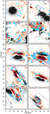 |
Fig. 6. Spatial distribution of all Hα Ellerman bomb detections (coloured crosses) for each data set (labelled in the top right of each panel) overlaid on HMI line-of-sight magnetograms, with positive (negative) polarity in red (black) and zero field strength in white. The cross colour is indicative of the event lifetime, ranging from cyan to purple for lifetimes between 0 and 15 min, with orange open diamonds for longer-lived events. The field-of-view in panel D is slightly shifted with respect to Fig. 1 to show all Hα detections and that the off-limb part of panel J has been manually set to zero. The magnetogram scales were byte-scaled independently. |
The 1735 detected Hα Ellerman bombs have average lifetimes about 3 min, with the lifetime distribution peaking closer to half of that but with a considerable tail out to about 15 min (third column of Table 4 and first panel of Fig. 5). About 6% of the Hα detections have longer lifetimes, unevenly spread up to over an hour, but 89% of the events have a lifetime of 10 min or less (these are total lifetimes within the detection constraints). They include re-brightenings and should not be taken to describe elemental Ellerman bomb features (i.e. substructure) which are known to vary on timescales of seconds or less (cf. Fig. 3 and the accompanying movie in Watanabe et al. 2011).
The average maximum area of the Hα-detected Ellerman bombs lies around 0.15 arcsec2. However, the area distributions (solid coloured outlined histograms in the second panel of Fig. 5) peak at small areas (0.05–0.1 arcsec2); the mean of the area minima per detection (dash-outlined, filled light grey overlay) peaks below 0.05 arcsec2. Ellerman bombs are truly sub-arcsecond features requiring the best telescope resolution presently available.
The peak contrasts (solid coloured outlined histograms in the third panel of Fig. 5) are measured as the maximum Hα intensity (the brightest pixel in all time steps showing the event) expressed as percentage brightening over the sequence-averaged mean intensity of the non-masked quiet parts of the field of view (Fig. 3). The average is close to 180%. The summed distribution shown by the purple histogram peaks in the 160–170% bin, close to the 169% average value over the mean contrast (not its peak but its mean over the detection lifetime) distribution shown by the filled dark grey overlay.
In the lifetime histograms in the first panel of Fig. 5 the individual data sets display rather similar behaviour, independent of viewing angle. Comparison with the second and third panels shows that where many short-lived events are detected (e.g. data sets C (light green), D (dark green) and F (red)), these are typically also on the small side and typically weaker in peak contrast. The scatter diagrams in the first two lower panels of Fig. 5 confirm the positive correlations of peak contrast with lifetime and area, with the latter somewhat tighter.
The last panel of Fig. 5 shows the variation of the mean values and the spread of the peak contrasts per data set ordered for viewing angle along the vertical μ axis. There is a slight trend to larger peak contrast towards the limb, with also larger spread. The mean peak contrasts reach up to 200% above the quiet-area average, much higher than typical mean contrasts (peak of the dark grey overlay in the upper panel).
Figure 6 shows the spatial distribution of all Hα detections overlaid on HMI line-of-sight magnetograms. The Ellerman bomb candidates in data sets A, B, E–I are mainly located in sunspot moat flows. In sets D and J they are concentrated between large assemblies of opposite-polarity fields. The longer-lived events (total lifetimes above 15 min, orange crosses) are predominantly found in areas showing more active-region complexity and/or flux emergence (e.g. sets C, D and J), or intense active-region decay (e.g. sets F and G).
4.2. AIA results
4.2.1. Performance for all Hα detections
Figures 7 and 8 summarise the AIA detection precision, recall and F1-score as function of imposed AIA brightness threshold for the individual data sets and averaged over all data sets, respectively. In each panel the two AIA passbands are distinguished with colour coding of the mean curves and of the spread that results from applying the different additional area and lifetime constraints in our grid of parameters. Figure 7 shows remarkable variations in curve behaviour between the different data sets. If all would peak at some optimum parameter combination our task would be easy, but this is not the case.
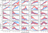 |
Fig. 7. AIA performance metrics precision P (top two rows, P-A–P-J), recall R (middle two rows, R-A–R-J) and the F1 score (bottom two rows, F1-A–F1-J) as function of the imposed AIA brightness threshold for data sets A–J (specified at top left per panel, in the top two rows with the number of Hα detections). In each panel the solid curves trace the averages for 1600 Å (blue) and 1700 Å (red), with correspondingly coloured shading (and darker overlaps) showing the spread per threshold that results from the different additional area and lifetime constraints in the AIA detection grid. The y-axis scales differ per panel. |
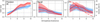 |
Fig. 8. Average performance metrics with respect to the Hα detections as function of the AIA brightness threshold: precision (left), recall (middle) and the F1-score (right). Colour coding as in Fig. 7. The dash-dotted curves in the third panel (scale at right) specify the recovery rates, i.e. the percentage of Hα detections with true-positive AIA detections, for the parameter combinations giving maximum F1 per threshold (peak of the F1 shading). |
FP errors come primarily from pseudo-EBs at low brightness, from FAFs at high brightness. Some FAFS do not pass our stationarity constraint by their fast apparent motion, but different amounts of remaining FAFs cause different divergences between the 1600 and 1700 Å metrics. Sets A, B, E, G show no or only few FAFs; sets C, I, and J have many.
Let us first consider the precision P, i.e. the TP fraction of all AIA detections (Eq. (1)). The top two rows (panels P-A–P-J) of Fig. 7 show that it generally increases with brightness threshold. For most data sets these increases are relatively smooth, but sets A and H are likely affected by their small-number statistics. These also show the lowest maximum P (note differences between P axis scales). The generally low P values at low threshold come from erroneous inclusion of pseudo-EBs. The starting values of the P curves are therefore lowest for fields of view that contain a large fraction of quiet-Sun (generally 70–80% but only around 50% for sets C, D and I). To reach high P a high AIA brightness threshold is required, generally 6–8σ over the quiet-area average or higher. A few cases then even reach 100% (blue curve for set E, red curve for G). In most panels the highest P values are reached with 1700 Å (red curve and shading) but sets B and E which contain no FAFs reach highest P in 1600 Å.
The middle two rows of Fig. 7 (panels R-A–R-J) depict the recall R, i.e. AIA’s recovery fraction of all Hα detections (Eq. (2)). It generally decreases with imposed AIA brightness threshold, as expected from the predominance of less bright Hα Ellerman bombs below the AIA resolution limit, and it reaches only values below 20% for most data sets. The behaviour of 1700 Å is more varied than for 1600 Å, showing steeper decreases in sets A and C and local maxima in B, I and J. The best performance (highest R reached at the upper border of the spread envelope) is better for data sets with fewer Hα detections (A, B, H), which may result from relative paucity of small and short-lived events that are harder for AIA to replicate.
The harmonic-mean F1-score in the bottom two rows of Fig. 7 (panels F1-A–F1-J) combines TP maximisation with FN and FP minimisation (Eq. (3)) and so mingles patterns in the corresponding P and R panels. Since the latter tend to opposite trends the resulting F1 values are generally poor. In some cases F1 seems almost independent of brightness threshold regardless of AIA diagnostic (e.g. sets C and D), while 1600 Å seems best in A and B and 1700 Å in I and J but not at the same brightness threshold. Roughly, F1 peaks at brightness thresholds between 5–7σ above the quiet average.
Figure 8 presents all-data averages of the three performance metrics weighted by the number of Hα-detections per data set. The recovery curves at right are similar to but reach higher than the recall curves in the centre panel, by holding for the best parameter combination instead of representing the average and because multiple Halpha Ellerman bombs may contribute to one true-positive AIA detection. In the last panel 1700 Å peaks at 5σ from balancing the opposite 1700 Å slopes in the first two panels. At this threshold the average 1700 Å recall is about 12%; the recovery for the best parameter combination including this threshold reaches over 19%. The corresponding precision P (not number-weighted as in the first panel but the total TP/(TP+FP) for the optimal parameter combination) is 27%.
When optimising instead for precision by using a 9σ threshold for 1700 Å then 62% of the 1700 Å detections are Hα Ellerman bombs but only 5% of the Hα population is recovered. This choice recovers only the tip of the iceberg.
4.2.2. Performance for Hα top fractions only
Previous studies have noted, although without statistical analysis, that typically the largest and brightest Hα Ellerman bombs overlap best with concentrated brightenings in the AIA images, as we find here when optimising P. Since the area distribution of the Hα detections in Fig. 5 peaks at small values below the 0.36 arcsec2 AIA pixel size, it is not surprising that AIA’s recovery is less than 20% at best and much smaller at higher thresholds. We therefore explore the possibility of obtaining higher recovery by considering only the top of the Hα population in terms of lifetime, area, and peak intensity, respectively. We also tested a fourth quantity, the total Ellerman bomb intensity obtained by summing the intensities in all its pixels over its entire lifetime, but found that this measure (a proxy for total released energy) does not give significantly better results.
Figure 9 shows AIA FN and TP distributions as function of the Hα Ellerman bomb lifetime, area and peak contrast with the goal to find how to separate FN and TP the best. They are summed over the two AIA diagnostics, using for each the parameter combination that yields the largest F1. The FN distributions show that most of the Hα detections that AIA missed are small. Compared to these the TP distributions have extended high-value tails; in each panel about half of the TPs fall above the dashed 30% boundary while only about 25–30% of the FNs do so. The best separation of the outer TP tail is for area; we therefore consider the top fractions in this quantity.
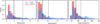 |
Fig. 9. Normalised distribution of AIA false negatives FN (red) and true positives TP (blue) as function of Hα Ellerman bomb lifetime, area, and peak contrast. Overlaps show up violet. The distributions are summations over the two AIA diagnostics, for each using the parameter combination yielding maximum F1, and are normalised by the total numbers specified in the first panel. The vertical lines indicate cut-offs for selecting the top 30% (dashed, N = 521) and 10% (dotted, N = 174) of the Hα Ellerman bombs for each quantity. |
Figure 10 presents these in the format of Fig. 8. The precision trends (first column) behave similar to Fig. 8 with the values still reaching about 60% and decreasing slightly for smaller sub-sample. AIA 1700 Å again outperforms 1600 Å above the 5σ threshold. The recall curves (centre column) now show a more pronounced peak for 1700 Å, extending to higher brightness threshold for smaller sub-sample, whereas those for 1600 Å are fairly constant with sub-sample size. The recall spread is of order 0.2–0.3, larger than in the centre panel of Fig. 8. The recall values increase significantly for smaller sub-sample size. AIA 1700 Å outperforms 1600 Å only marginally below brightness threshold 6–7σ, while 1600 Å does better above 8σ. In the F1-scores (third column) 1700 Å again outperforms 1600 Å, peaking at 6–7σ for the top 30% sub-sample and at 7–8σ for the top 10% sub-sample. However, lower brightness thresholds yield better recovery rates (dot-dashed curves, axis at right), with little difference between 1600 Å and 1700 Å below 7σ.
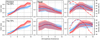 |
Fig. 10. Average metrics performance as function of AIA brightness threshold for only the top 30% and 10% Hα detections in terms of area. Format as for Fig. 8. |
When optimising for F1 by selecting the 1700 Å 7σ threshold both P and R are higher than for the F1-optimised full Hα population but still below 50%, while the recovery percentage of all Hα detections (from the full population) becomes only 5–8%. When optimising for P by selecting the 9σ threshold the recovery drops further to 3–5%. The conclusion is that this sub-class selection does not improve the metrics performances dramatically, while still recovering less than half of the sub-sample.
4.3. Optimal AIA results
4.3.1. Optimal detection parameters
Since our trials using only top Hα detections did not produce significantly better metrics we define optimal criteria from the results for all Hα detections that were summarised in Fig. 8. On their basis we only employ the 1700 Å images. For F1 maximisation the criteria are: (1) an intensity threshold of 5σ above the quiet-area average, (2) an area between 1–18 AIA pixels, and (3) a minimum lifetime of 1 min without upper limit. The corresponding metric values are P = 27%, R = 19%, F1 = 0.23. If one prefers to instead optimise precision P the first two criteria become: intensity threshold 9σ above the average and area 1–9 AIA pixels. The lifetime condition remains the same. The metrics then become P = 62%, R = 5%, F1 = 0.09. Table 5 summarises the TP, FP and FN counts for both F1 and P optimisation.
Detection numbers in Hα and AIA 1700 Å.
4.3.2. Properties of AIA-detected Ellerman bombs
Figure 11 shows statistical properties of the AIA detections resulting from both optimisation recipes, colour-split between true positives TP and false negatives FP and also splitting F1 maximisation (filled histograms and symbols) and P maximisation (open histograms and symbols). The lack of detections above 3.5 arcsec2 for the P-maximised area histograms (outlined) is imposed by the upper area limit of 9 AIA pixels. Comparison with the Hα-Ellerman bomb statistics in Fig. 5 shows that the TPs have similar lifetime (upper left panels in the two figures) and brightness (upper right panels) distributions, but a different area distribution (upper centre panels).
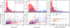 |
Fig. 11. AIA 1700 Å detection statistics as function of properties. Figure layout as for Fig. 5, except that in all but the last panel distinction is made between true positives TP (AIA detection with Hα detection) and false positives FP (AIA detection without Hα detection) rather than data sets. The peak contrasts are given as percentage above the intensity threshold (quiet-Sun average +5σ for F1 maximisation, +9σ for P maximisation). Upper row: each panel shows the TP (blue and purple) and FP (red) distribution distributions for the parameter combination maximising F1 (filled histograms) and P (outlined histograms). Lower row: as Fig. 5 but the symbols in the two scatter plots are colour-coded between TP and FP as in the upper row, and with distinction between F1 maximisation (filled circles) and P maximisation (open circles). The last panel shows average peak contrasts for the TP detections with the bar lengths showing the rms spreads around the indicated mean values and with similar distinction between maximising F1 (filled circles and solid lines) and maximising P (open circles and dotted lines). The total TP and FP numbers are given in the top right of the first panel, with slash-separation between F1 and P maximisation. The vertical and horizontal dashed grey lines in all but the last panel indicate the threshold values for sub-selection of the top 10% longest-lived, largest and brightest events. |
The average lifetime and brightness are larger than for Hα because AIA favours larger features that tend to be brighter and live longer. We find lifetimes of the order of 5 ± 7 min for both F1- and P-maximised detection populations. The TP and FP lifetime distributions also differ between the two maximisations, with TPs peaking at lifetimes about 9 min and 6 min, respectively, but FPs at about 3–4 min for both. Although there is no strong correlation with the intensity contrast (lower left panel) and many TPs are as faint and short-lived as the majority of the FPs, the fraction of TPs among the longer-lived events is larger, with higher contrasts. For example, there are no TP detections lasting 15 min with brightness contrast below 125%.
The FP area distribution (upper centre panel) shows a broad peak with most FP detections below 2 arcsec2 regardless of maximisation, while part of the TPs has similarly small areas and their majority exceeds 2 arcsec2. As for the Hα Ellerman bombs, the first two lower panels show higher correlation between detection area and brightness contrast than for lifetime. In particular, there are no detections smaller than 1 arcsec2 with a contrast above 150% of the mean, whereas there are several detections above that contrast that last only 2 min or less.
The third panel shows that for both F1 and P maximisation the FPs are mostly below 130% (90% and 80% of their numbers) while nearly half of the TPs are higher. The panel underneath shows a tendency for the F1-maximised sample to have lower contrast closer to the limb, less for the P-maximised detections (open circles).
4.3.3. Performance for AIA top fractions only
Finally, the precision can be optimised further by recognising that the false positives FP in Fig. 11 cluster at shorter lifetimes, smaller areas and lower contrasts so that they can be largely avoided by dropping these samplings altogether. For using the F1 criteria we perform this additional selection by maintaining only those AIA detections that (1) have a lifetime longer than 20 AIA frames (8 min), (2) are larger than 7 AIA pixels (2.52 arcsec2) and (3) show peak contrast larger than 135% of the 5σ-over-average threshold (9σ in the case of the P-maximised population). Together these outer-tail selections imply maintaining the top ∼10% of all AIA detections. We found that then the probability that a remaining AIA detection is an Hα Ellerman bomb increases from 27% to 80%. Using the same thresholds on P-maximised detections increases the hit rate even to 87%.
5. Discussion
5.1. Hα criteria
Our final detection criteria for Hα Ellerman bomb detection are: (1) a double core–halo intensity threshold at 145% and 130% of the quiet-Sun average determined from masked HMI data (i.e. a core of pixels with brightness of at least 145%; the halo consists of pixels of at least 130% that are adjacent to the core or to other halo pixels) in either the blue or red wing-average images (constructed from averaging over ±(0.9–1.1) Å) or both, (2) an area threshold of 0.035 arcsec2, and (3) a lifetime threshold of approximately 1 min.
Both intensity thresholds are lower than the ones used by Vissers et al. (2015a) from normalisation to quiet-Sun sub-field averaging rather then full field-of-view averaging. The same thresholds were employed by Reid et al. (2016) and they are similar to those of Watanabe et al. (2011) and Zachariadis et al. (1987).
For the area threshold we tested values ranging from 5 to 20 SST pixels (0.018–0.070 arcsec2) but found through our CRISPEX inspections that a 5 pix (0.018 arcsec2) constraint delivered too many dubious detections whereas for 15–20 pix too many valid events were excluded. We therefore settled on 10 pix (0.035 arcsec2) which lies between the 0.05–0.11arcsec2 of Reid et al. (2016) and Chen et al. (2017), and the ∼0.015–0.02 arcsec2 value used in e.g. Vissers et al. (2013, 2015a), Nelson et al. (2015).
In our Hα data the main culprits causing missing or wrong Ellerman bomb identification are too low cadence and too large or too long seeing deteriorations. In addition, the SST resolution sets a lower limit to detectable Ellerman bomb area; it may well be that additional photospheric reconnection events exist that are even smaller and weaker than the tiny QSEBs of Rouppe van der Voort et al. (2016), but if so these are unlikely to be picked up at any other optical telescope nor with AIA (which does not show QSEBs in its ultraviolet images).
5.2. Hα detections
Both the Hα-detection lifetime range (majority between 1 and 15 min) and its average (roughly 3 min) compare well with earlier high-resolution SST studies (cf. Fig. 5). Vissers et al. (2013) report an average of 3.5–4 min with 75% of the Ellerman bomb detections having lifetimes shorter than 5 min, Nelson et al. (2015) find lifetimes between 3–20 min with 7 min average and Reid et al. (2016) note lifetimes ranging 0.5–14 min peaking around 1 min. The typical areas found here (majority between 0.035 and 0.4 arcsec2, average 0.14 arcsec2) are rather small; both Vissers et al. (2013) and Nelson et al. (2015) find averages about 0.2–0.3 arcsec2. Earlier Zachariadis et al. (1987) had found 0.6 arcsec2. Reid et al. (2016) report much larger areas but actually found very similar values with the majority in the range of 0.06–0.21 arcsec2 (priv. comm.).
We find positive correlation between lifetime and peak intensity contrast and a stronger correlation between detection area and intensity contrast (cf. first two lower panels of Fig. 5), similar to e.g. Nelson et al. (2015), Libbrecht et al. (2017), Chen et al. (2017).
5.3. AIA 1700 Å detections
Only few statistics exist in the literature regarding Ellerman bomb-related detections in mid-ultraviolet continua. Vissers et al. (2013) report 1.1–1.3 arcsec2 average for features detected using a 5σ-above-mean threshold in AIA 1700 Å (without area constraint other than a 0.36 arcsec2 lower limit), somewhat lower than our average of 1.94 ± 1.75 arcsec2 for the total population including both true and false positives. Pariat et al. (2007) found the majority of Ellerman bomb-related brightenings identified in similar 1600 Å images from the Transition Region and Coronal Explorer (TRACE) to have lifetimes between 1.5 and 7 min, with an average at 3.5 min. Our true-positive population shows a much higher average of just over 8 min, but also a large spread with median lifetime only 3.8 min.
The recent statistical study by Chen et al. (2017) used a 3.5σ above average brightness threshold. Although they do not report feature sizes, they do note that above a lifetime of 20 min AIA-detected Ellerman bombs dominate their population of AIA 1700 Å detections. In our case, this tipping point lies at only 5.5 min, with respectively 68% and 79% of the AIA detections being true positives when considering lifetimes above 10 and 20 min, but this difference may be explained by the positive correlation between areas and lifetime and noting that Chen et al. (2017) used a 4 AIA-pixel lower limit. While not specifically targeting Ellerman bombs, Toriumi et al. (2017) used a 5σ threshold in 1700 Å to select events for comparison with Ca II H bright points in an emerging flux region; the authors argued (and we agree) that many of those were likely Ellerman bombs.
5.4. Viewing angle effects
Ellerman bomb detection sensitivity to viewing angle may be expected. On the one hand, Ellerman bombs are easier recognised towards the limb through higher contrast (last panel of Fig. 5) and because their projected area increases (e.g. data set A versus E). On the other hand, foreshortening at smaller μ reduces the projected size of active regions so that more quiet Sun comes into view (as in sets H and J in Fig. 1).
We find no clear trend with viewing angle (data set order) in the lifetimes and maximum detection areas in Table 4. There is a hint of increasing average peak contrast at more limb-ward viewing (last panel of Fig. 5), but the standard deviations are too large to make this significant. Variations in the inherent activity and evolutionary stage of the observed target may be more important. For instance, data set C exhibits an excessively high detection rate, but this target was part of a highly complex active region with increasing flux emergence during the time of our observations. Similarly, sets H and A (sampling the same active region on 27 June and 2 July 2010) had similar detection rates even though the viewing angle differed over 0.5.
5.5. How suitable are AIA 1700 Å images to detect Ellerman bombs?
Ideally, our efforts would have produced a recipe that recovers Hα Ellerman bombs one-to-one from AIA data. However, as demonstrated in Figs. 7–8 it is not possible to exclude false detections when optimising F1 since neither precision nor recall then reach unity; optimising for precision alone does better in that quantity but recovers fewer Hα-Ellerman bombs. The result above is that F1 optimisation reaches only 27% precision (AIA detections that correspond to Hα detections) and 19% recall (Hα detections recovered by AIA), and that these percentages become 62% and 5% when optimising precision (Sect. 4.3). High recovery was only reached in the subsequent top-10% AIA selection.
This lack of one-to-one correspondence has been noted before. Previous studies found ultraviolet recoveries of Hα Ellerman bombs over 50% (Qiu et al. 2000; Georgoulis et al. 2002, higher than our results but from Hα observations with worse angular resolution. When we discard Hα detections below 0.64 arcsec2 (the pixel size in the second study) we obtain a recovery of 66% (cf. Figs. 9 and 10).
The recent study by Chen et al. 2017 found precision 53% and recall 51%. Applying their area thresholds of 0.11 arcsec2 (three times ours) for Hα and 1.44 arcsec2 (four times ours) for AIA gives precision 44% and recall 22% in our results, but we suspect that the first threshold was below the effective resolution.
Moreover, false detections are inevitable. They are partly explained by the ten-fold resolution difference between the SST and AIA since the majority of the maximum Hα Ellerman bomb areas in Fig. 5 is smaller than one AIA pixel of 0.36 arcsec2 (Fig. 5). A large class of potential false detections consists of pseudo-EBs marking magnetic concentrations in quiescent network.
In addition, there is no reason per se to presume that all Hα-observed Ellerman bombs have counterparts in the ultraviolet. Several observational studies (Vissers et al. 2015a; Kim et al. 2015; Tian et al. 2016; Libbrecht et al. 2017) have demonstrated that while the Ellerman bomb and UV burst populations overlap, they do not do so entirely; recent simulation results suggest that the non-overlaps are at higher reconnection height (Hansteen et al. 2017). Hence, false positives may correspond to UV bursts without Ellerman bomb counterpart (Vissers et al. 2015a). While regrettable from the perspective of identifying pure Ellerman bombs, these may also serve to trace low-atmosphere reconnection and provide early warning of emerging flux. Our final suggestion to consider only the top 10% fraction of AIA detections, giving 80% Ellerman bomb recall excluding all pseudo-EBs, likely includes these in the remaining 20% and so may well deliver such candidates additionally.
6. Conclusion
We implemented Ellerman bomb detection recipes for both imaging spectroscopy in Hα and mid-ultraviolet imaging with AIA that improve on earlier versions. Key improvements are to consider the Hα±(0.9–1.1) Å wings separately and the definition of viewing-angle and data-set independent quiet-Sun-passing masks to define brightness thresholds.
We thus detected 1735 Ellerman bombs in high-quality Hα observations with the SST of active regions at ten locations that together span centre-to-limb viewing and active-region variation. This is the first study sampling many Ellerman bombs from multiple active regions. The large variations in Figs. 5 and 7 show that using only a few in a single observation to address their visibility in different diagnostics and their role in the energy and mass budget of the outer atmosphere, as was done in a number of studies including recent ones, may yield skewed results and should be done with great care.
We inventoried the corresponding appearance and detectability in simultaneous AIA 1600 and 1700 Å images. With a completeness analysis applying a detection-parameter grid to these we derived optimal detection criteria to either recover the largest fraction of Hα-Ellerman bombs while minimising false detections, or to maximise the number of AIA-detections that are Hα-Ellerman bombs. Whether to prioritise the one or the other is a choice that depends on the purpose of the study.
Overall, detection in AIA 1700 Å yields the best results. Our recommended detection criteria for this diagnostic and the first choice in prioritising are:
-
minimum brightness threshold of 5σ above the local quiet-Sun average obtained with masks derived from HMI data;
-
area limit to between 1 and 18 AIA pixels (0.4–6.5 arcsec2);
-
minimum lifetime threshold of 1 min.
These parameter choices should recover about 20% of the Hα-Ellerman bomb population, while ensuring that nearly 30% of the AIA detections is indeed an Hα-Ellerman bomb. Optimising instead for detection precision by using 9σ brightness threshold and 1–9 pix area constraint makes over 60% of the AIA events Hα-detected Ellerman bombs, but at the cost of recovering only about 5% of all Hα Ellerman bombs.
Further restriction to only the top 10% fraction of all AIA detections that result from the three criteria above can be done by using additional combined thresholds for lifetime (20 AIA frames), area (7 AIA pixels) and peak contrast (above 135% of the 5σ value). This reaches over 80% probability that each remaining AIA detection was an Hα-observable Ellerman bomb.
Ellerman bomb detection in the AIA mid-UV images is thus feasible and can recover a significant fraction of Hα Ellerman bombs, although full recovery of the complete Hα-Ellerman bomb population that is detectable at the high resolution and quality of the SST cannot be achieved with the low-resolution AIA images. A fortiori, the smaller but still Ellerman-like QSEB reconnection events are not observed in AIA’s ultraviolet passbands (Rouppe van der Voort et al. 2016). However, the top 10% AIA selection furnishes a secure way of finding the more important ones and while the recall is then low, some applications (e.g. early detection of flux emergence or of active region formation) may not require this but still benefit from the high precision in AIA detection of Ellerman bombs. In addition, most of the then remaining 20% false positive detections are probably UV burst candidates without Ellerman bomb counterpart but of interest in their own right as marking higher-up reconnection.
Altogether, our recipe opens the entire AIA database for performing continuous, full-disc detection and tracking of low-atmosphere reconnection events and thereby of flux emergence and magnetic active region evolution in the past or at present. For example, such monitoring may provide valuable input in flare forecasting.
Acknowledgments
Our research was supported under the CHROMOBS grant by the Knut and Alice Wallenberg Foundation, as well as by the ERC under the European Union’s Seventh Framework Programme (FP7/2007-2013)/ERC grant agreement nr. 291058. This research was also supported by the Research Council of Norway, project number 250810, and through its Centres of Excellence scheme, project number 262622. The Swedish 1 m Solar Telescope is operated on the island of La Palma by the Institute for Solar Physics of Stockholm University in the Spanish Observatorio del Roque de los Muchachos of the Instituto de Astrofísica de Canarias. We are grateful to Eamon Scullion for kindly providing the Hα data of June 20, 2012. We also want to thank Patrick Antolin, Mats Carlsson, Jaime de la Cruz Rodríguez, Ainar Drews, Viggo Hansteen, Shahin Jafarzedeh, Torben Leifsen, Ada Ortiz, Tiago Pereira and Mikolaj Szydlarski for contributing to the other SST observations used here. This work benefited from discussions at the meetings “Solar UV bursts – a new insight to magnetic reconnection” at the International Space Science Institute (ISSI) in Bern. We made much use of NASA’s Astrophysics Data System Bibliographic Services. We also acknowledge the community effort to develop open-source packages used here: numpy (numpy.org), matplotlib (matplotlib.org), sunpy (sunpy.org).
References
- Archontis, V., & Hood, A. W. 2009, A&A, 508, 1469 [NASA ADS] [CrossRef] [EDP Sciences] [Google Scholar]
- Berger, T. E., Rouppe van der Voort, L. H. M., & Löfdahl, M. G. 2004, A&A, 428, 613 [NASA ADS] [CrossRef] [EDP Sciences] [Google Scholar]
- Berlicki, A., Heinzel, P., & Avrett, E. H. 2010, Mem. Soc. Astron. It., 81, 646 [NASA ADS] [Google Scholar]
- Chen, Y., Tian, H., Xu, Z., et al. 2017, Geosci. Lett., 4, 30 [NASA ADS] [CrossRef] [Google Scholar]
- Danilovic, S. 2017, A&A, 601, A122 [NASA ADS] [CrossRef] [EDP Sciences] [Google Scholar]
- de la Cruz Rodríguez, J., Löfdahl, M. G., Sütterlin, P., Hillberg, T., & Rouppe van der Voort, L. 2015, A&A, 573, A40 [NASA ADS] [CrossRef] [EDP Sciences] [Google Scholar]
- De Pontieu, B., Title, A. M., Lemen, J. R., et al. 2014, SoPh, 289, 2733 [NASA ADS] [Google Scholar]
- Díaz Baso, C. J., & Asensio Ramos, A. 2018, A&A, 614, A5 [NASA ADS] [CrossRef] [EDP Sciences] [Google Scholar]
- Ellerman, F. 1917, ApJ, 46, 298 [NASA ADS] [CrossRef] [Google Scholar]
- Fang, C., Tang, Y. H., Xu, Z., Ding, M. D., & Chen, P. F. 2006, ApJ, 643, 1325 [NASA ADS] [CrossRef] [Google Scholar]
- Georgoulis, M. K., Rust, D. M., Bernasconi, P. N., & Schmieder, B. 2002, ApJ, 575, 506 [NASA ADS] [CrossRef] [Google Scholar]
- Grubecka, M., Schmieder, B., Berlicki, A., et al. 2016, A&A, 593, A32 [NASA ADS] [CrossRef] [EDP Sciences] [Google Scholar]
- Hansteen, V. H., Archontis, V., Pereira, T. M. D., et al. 2017, ApJ, 839, 22 [NASA ADS] [CrossRef] [Google Scholar]
- Harvey, K., & Harvey, J. 1973, Sol. Phys., 28, 61 [NASA ADS] [CrossRef] [Google Scholar]
- Hashimoto, Y., Kitai, R., Ichimoto, K., et al. 2010, PASJ, 62, 879 [NASA ADS] [Google Scholar]
- Herlender, M., & Berlicki, A. 2011, Cent. Eur. Astrophys. Bull., 35, 181 [NASA ADS] [Google Scholar]
- Kim, Y.-H., Yurchyshyn, V., Bong, S.-C., et al. 2015, ApJ, 810, 38 [NASA ADS] [CrossRef] [Google Scholar]
- Leenaarts, J., Rutten, R. J., Carlsson, M., & Uitenbroek, H. 2006a, A&A, 452, L15 [NASA ADS] [CrossRef] [EDP Sciences] [Google Scholar]
- Leenaarts, J., Rutten, R. J., Sütterlin, P., Carlsson, M., & Uitenbroek, H. 2006b, A&A, 449, 1209 [NASA ADS] [CrossRef] [EDP Sciences] [Google Scholar]
- Libbrecht, T., Joshi, J., Rodríguez, J. D. L. C., Leenaarts, J., & Ramos, A. A. 2017, A&A, 598, A33 [NASA ADS] [CrossRef] [EDP Sciences] [Google Scholar]
- Löfdahl, M. G., Hillberg, T., de la Cruz Rodriguéz, J., et al. 2018, ArXiv e-prints [arXiv:1804.03030] [Google Scholar]
- Matsumoto, T., Kitai, R., Shibata, K., et al. 2008, PASJ, 60, 577 [NASA ADS] [CrossRef] [Google Scholar]
- Nelson, C. J., Doyle, J. G., Erdélyi, R., et al. 2013, Sol. Phys., 283, 307 [NASA ADS] [CrossRef] [Google Scholar]
- Nelson, C. J., Scullion, E. M., Doyle, J. G., Freij, N., & Erdélyi, R. 2015, ApJ, 798, 19 [NASA ADS] [CrossRef] [Google Scholar]
- Pariat, E., Schmieder, B., Berlicki, A., et al. 2007, A&A, 473, 279 [NASA ADS] [CrossRef] [EDP Sciences] [Google Scholar]
- Peter, H., Tian, H., Curdt, W., et al. 2014, Science, 346, 1255726 [NASA ADS] [CrossRef] [Google Scholar]
- Qiu, J., Ding, M. D., Wang, H., Denker, C., & Goode, P. R. 2000, ApJ, 544, L157 [NASA ADS] [CrossRef] [Google Scholar]
- Reardon, K., Tritschler, A., & Katsukawa, Y. 2013, ApJ, 779, 143 [NASA ADS] [CrossRef] [Google Scholar]
- Reid, A., Mathioudakis, M., Scullion, E., et al. 2015, ApJ, 805, 64 [NASA ADS] [CrossRef] [Google Scholar]
- Reid, A., Mathioudakis, M., Doyle, J. G., et al. 2016, ApJ, 823, 110 [NASA ADS] [CrossRef] [Google Scholar]
- Rezaei, R., & Beck, C. 2015, A&A, 582, A104 [NASA ADS] [CrossRef] [EDP Sciences] [Google Scholar]
- Rouppe van der Voort, L. H. M., Rutten, R. J., & Vissers, G. J. M. 2016, A&A, 592, A100 [NASA ADS] [CrossRef] [EDP Sciences] [Google Scholar]
- Rouppe van der Voort, L., De Pontieu, B., & Scharmer, G. B. 2017, ApJ, 851, L6 [NASA ADS] [CrossRef] [Google Scholar]
- Rutten, R. J. 2016, A&A, 590, A124 [NASA ADS] [CrossRef] [EDP Sciences] [Google Scholar]
- Rutten, R. J., Vissers, G. J. M., Rouppe van der Voort, L. H. M., Sütterlin, P., & Vitas, N. 2013, J. Phys. Conf. Ser., 440, 012007 [NASA ADS] [CrossRef] [Google Scholar]
- Rutten, R. J., Rouppe van der Voort, L. H. M., & Vissers, G. J. M. 2015, ApJ, 808, 133 [NASA ADS] [CrossRef] [Google Scholar]
- Scharmer, G. B., Bjelksjo, K., Korhonen, T. K., Lindberg, B., & Petterson, B. 2003a, in Innovative Telescopes and Instrumentation for Solar Astrophysics, eds. S. L. Keil, & S. V. Avakyan, Proc. SPIE, 4853, 341 [NASA ADS] [CrossRef] [Google Scholar]
- Scharmer, G. B., Dettori, P. M., Löfdahl, M. G., & Shand, M. 2003b, in Innovative Telescopes and Instrumentation for Solar Astrophysics, eds. S. L. Keil, & S. V. Avakyan, Proc. SPIE, 4853, 370 [NASA ADS] [CrossRef] [Google Scholar]
- Scharmer, G. B., Narayan, G., Hillberg, T., et al. 2008, ApJ, 689, L69 [NASA ADS] [CrossRef] [Google Scholar]
- Socas-Navarro, H., Martínez Pillet, V., Elmore, D., et al. 2006, Sol. Phys., 235, 75 [NASA ADS] [CrossRef] [Google Scholar]
- Tian, H., Xu, Z., He, J., & Madsen, C. 2016, ApJ, 824, 96 [NASA ADS] [CrossRef] [Google Scholar]
- Title, A. M., & Berger, T. E. 1996, ApJ, 463, 797 [NASA ADS] [CrossRef] [Google Scholar]
- Toriumi, S., Katsukawa, Y., & Cheung, M. C. M. 2017, ApJ, 836, 63 [NASA ADS] [CrossRef] [Google Scholar]
- van Noort, M., Rouppe van der Voort, L., & Löfdahl, M. G. 2005, Sol. Phys., 228, 191 [NASA ADS] [CrossRef] [Google Scholar]
- Vernazza, J. E., Avrett, E. H., & Loeser, R. 1981, ApJS, 45, 635 [NASA ADS] [CrossRef] [Google Scholar]
- Vissers, G., & Rouppe van der Voort, L. 2012, ApJ, 750, 22 [NASA ADS] [CrossRef] [Google Scholar]
- Vissers, G. J. M., Rouppe van der Voort, L. H. M., & Rutten, R. J. 2013, ApJ, 774, 32 [NASA ADS] [CrossRef] [Google Scholar]
- Vissers, G. J. M., Rouppe van der Voort, L. H. M., Rutten, R. J., Carlsson, M., & De Pontieu, B. 2015a, ApJ, 812, 11 [NASA ADS] [CrossRef] [Google Scholar]
- Vissers, G. J. M., Rouppe van der Voort, L. H. M., & Carlsson, M. 2015b, ApJ, 811, L33 [NASA ADS] [CrossRef] [Google Scholar]
- Vissers, G. J. M., de la Cruz Rodríguez, J., Libbrecht, T., et al. 2019, A&A, accepted [arXiv:1905.02035] [Google Scholar]
- Watanabe, H., Vissers, G., Kitai, R., Rouppe van der Voort, L., & Rutten, R. J. 2011, ApJ, 736, 71 [NASA ADS] [CrossRef] [Google Scholar]
- Young, P. R., Tian, H., Peter, H., et al. 2018, Space Sci. Rev., 214, 120 [NASA ADS] [CrossRef] [Google Scholar]
- Zachariadis, T. G., Alissandrakis, C. E., & Banos, G. 1987, Sol. Phys., 108, 227 [NASA ADS] [CrossRef] [Google Scholar]
All Tables
Hα intensity, area and lifetime thresholds for Ellerman bomb selection and resulting detection rates in recent literature.
All Figures
|
Fig. 1. Full field-of-view samples of all 10 data sets. Panel pairs (A)–(J) show near-simultaneous co-aligned CRISP Hα-wing images (orange; blue-wing images averaged around −1 Å for all but data set B that shows the red wing at +1 Å) and AIA 1700 Å images (red-brown), ordered by decreasing viewing angle μ (= cos θ, with θ the angle between the line-of-sight and the normal to the solar surface) specified at lower-left in each AIA panel with the image-centre solar (X, Y) location. The times of the SST observations are specified at lower-left in each CRISP panel. The corresponding AIA image cutouts were interpolated to these from their 24 s sampling cadence (through nearest-neighbour frame selection) and rotated to the SST orientation. Each field of view has been cut slightly to obtain the same display size and scale. The arrows at top left in each AIA panel point towards solar north (red), west (blue) and the nearest limb (white). Each image is byte-scaled independently including high-level clipping to improve the overall scene visibility. Dashed frames in pairs C, D, F and I define cutouts for Fig. 2, solid frames in pair E define cutouts for Fig. 4. |
| In the text | |
|
Fig. 2. Feature visibilities in AIA 1600 Å (first and third columns) and 1700 Å (second and fourth columns). The panel pairs show selected cutouts for data sets A, C, D, F, H and I, labelled with their μ values in the 1600 Å panels. The cutout locations are outlined by dashed frames in the corresponding panels of Fig. 1. In order to accommodate the dynamic range the square root of the intensity is shown. The byte scaling is common between pairs and is defined so that quiet areas obtain the same apparent average brightness in 1600 and 1700 Å at a scale that saturates at 15σ above this quiet average for 1700 Å except for set F where 10σ was used to for better display contrast. At these values no 1700 Å image is clipped; only the brightest 1600 Å features are. The blue contours outline 1700 Å areas at least 5σ above the quiet average. Major tick marks are spaced 10″ apart, minor tick marks 2″ as in Fig. 1. |
| In the text | |
|
Fig. 3. HMI mask construction for data sets A (viewing angle μ = 0.93, top row) and I (μ = 0.36, bottom row). The masks serve to define the local quiet area for reference brightness thresholding. Left to right: HMI continuum image, HMI line-of-sight magnetogram (positive polarity in red, negative in black, zero field strength white), AIA 1700 Å image, blue wing Hα image. The HMI intensity mask is outlined by blue contours in the first column, the HMI magnetic field mask by green contours in the second column. The composite mask is shown in all panels by purple dashed contours. The small green-only islands in the second column are blocked by the minimum-area constraint. In the last panel the blocked part covers most of the upper half including all Ellerman bombs. |
| In the text | |
|
Fig. 4. Examples of detection evaluations from data set E. The two panel pairs show Hα−(0.9–1.1) Å blue-wing average intensity and AIA 1700 Å intensity for the similarly numbered cutouts in panel pair E of Fig. 1. Detection contours in Hα (cyan and orange) and AIA 1700 Å (blue and red; 5σ threshold, minimum of 1 AIA px and 2 frames visibility) are overlaid. The blue AIA contours (all panels) are classified as true positive (TP) detections from their degree of overlap with the cyan Hα contours (first and third panel), whereas the red contour in the first panel pair shows a false positive (FP), the orange contours in the second panel pair two false negatives (FN). |
| In the text | |
|
Fig. 5. Statistics of all 1735 Ellerman bomb detections in Hα. In all panels the ten different data sets are colour-coded blue-green-red-orange-purple along increasing viewing angle (decreasing μ); see also the top middle panel for the colour-correspondence of each data set A–J. Upper row: stacked occurrence histograms as function of lifetime, maximum area, and contrast. The histogram bin sizes are 1 min, 0.05 arcsec2, and 10%. Since the coloured histograms are stacked the topmost dark purple ones also outline the cumulative distributions. The dark grey and dash-outlined, light grey overlays in the second and third panels show the cumulative distributions for the mean and minimum area and contrast over the lifetime of each detection, respectively. These grey overlay histograms have been scaled down by a factor 3 in height to fit on the same scale as the coloured histograms. Lower row: scatter plots of peak contrast as function of lifetime and maximum area. The last panel shows peak contrasts at the different μ values, with the bar lengths showing the rms peak contrast spreads around their mean values shown by the dots. |
| In the text | |
|
Fig. 6. Spatial distribution of all Hα Ellerman bomb detections (coloured crosses) for each data set (labelled in the top right of each panel) overlaid on HMI line-of-sight magnetograms, with positive (negative) polarity in red (black) and zero field strength in white. The cross colour is indicative of the event lifetime, ranging from cyan to purple for lifetimes between 0 and 15 min, with orange open diamonds for longer-lived events. The field-of-view in panel D is slightly shifted with respect to Fig. 1 to show all Hα detections and that the off-limb part of panel J has been manually set to zero. The magnetogram scales were byte-scaled independently. |
| In the text | |
|
Fig. 7. AIA performance metrics precision P (top two rows, P-A–P-J), recall R (middle two rows, R-A–R-J) and the F1 score (bottom two rows, F1-A–F1-J) as function of the imposed AIA brightness threshold for data sets A–J (specified at top left per panel, in the top two rows with the number of Hα detections). In each panel the solid curves trace the averages for 1600 Å (blue) and 1700 Å (red), with correspondingly coloured shading (and darker overlaps) showing the spread per threshold that results from the different additional area and lifetime constraints in the AIA detection grid. The y-axis scales differ per panel. |
| In the text | |
|
Fig. 8. Average performance metrics with respect to the Hα detections as function of the AIA brightness threshold: precision (left), recall (middle) and the F1-score (right). Colour coding as in Fig. 7. The dash-dotted curves in the third panel (scale at right) specify the recovery rates, i.e. the percentage of Hα detections with true-positive AIA detections, for the parameter combinations giving maximum F1 per threshold (peak of the F1 shading). |
| In the text | |
|
Fig. 9. Normalised distribution of AIA false negatives FN (red) and true positives TP (blue) as function of Hα Ellerman bomb lifetime, area, and peak contrast. Overlaps show up violet. The distributions are summations over the two AIA diagnostics, for each using the parameter combination yielding maximum F1, and are normalised by the total numbers specified in the first panel. The vertical lines indicate cut-offs for selecting the top 30% (dashed, N = 521) and 10% (dotted, N = 174) of the Hα Ellerman bombs for each quantity. |
| In the text | |
|
Fig. 10. Average metrics performance as function of AIA brightness threshold for only the top 30% and 10% Hα detections in terms of area. Format as for Fig. 8. |
| In the text | |
|
Fig. 11. AIA 1700 Å detection statistics as function of properties. Figure layout as for Fig. 5, except that in all but the last panel distinction is made between true positives TP (AIA detection with Hα detection) and false positives FP (AIA detection without Hα detection) rather than data sets. The peak contrasts are given as percentage above the intensity threshold (quiet-Sun average +5σ for F1 maximisation, +9σ for P maximisation). Upper row: each panel shows the TP (blue and purple) and FP (red) distribution distributions for the parameter combination maximising F1 (filled histograms) and P (outlined histograms). Lower row: as Fig. 5 but the symbols in the two scatter plots are colour-coded between TP and FP as in the upper row, and with distinction between F1 maximisation (filled circles) and P maximisation (open circles). The last panel shows average peak contrasts for the TP detections with the bar lengths showing the rms spreads around the indicated mean values and with similar distinction between maximising F1 (filled circles and solid lines) and maximising P (open circles and dotted lines). The total TP and FP numbers are given in the top right of the first panel, with slash-separation between F1 and P maximisation. The vertical and horizontal dashed grey lines in all but the last panel indicate the threshold values for sub-selection of the top 10% longest-lived, largest and brightest events. |
| In the text | |
Current usage metrics show cumulative count of Article Views (full-text article views including HTML views, PDF and ePub downloads, according to the available data) and Abstracts Views on Vision4Press platform.
Data correspond to usage on the plateform after 2015. The current usage metrics is available 48-96 hours after online publication and is updated daily on week days.
Initial download of the metrics may take a while.