| Issue |
A&A
Volume 625, May 2019
|
|
|---|---|---|
| Article Number | A145 | |
| Number of page(s) | 11 | |
| Section | Planets and planetary systems | |
| DOI | https://doi.org/10.1051/0004-6361/201935349 | |
| Published online | 28 May 2019 | |
Transit-period search from single-event space-based data: the role of wide-field surveys
Konkoly Observatory of the Hungarian Academy of Sciences, Konkoly Thege ut. 15-17, Budapest 1121, Hungary
e-mail: kovacs@konkoly.hu
Received:
23
February
2019
Accepted:
15
April
2019
We investigate the optimization of dataset weighting in searching for the orbital period of transiting planets when high-precision space-based data with a single transit event are combined with (relatively) low-precision ground-based (wide-field) data. The optimization stems from the lack of multiple events in the high-precision data and the likely presence of such events in the low-precision data. With noise minimization, we combined two types of frequency spectra: (i) spectra that use two fixed transit parameters (moment of the center of the transit and duration of the event) derived from the space data alone; (ii) spectra that result from the traditional weighted box signal search with optimized transit parameters for each trial period. We used many mock signals to test the detection power of the method. Marginal or no detections in the ground-based data may lead to secure detections in the combined data with the above weighting. Depending on the coverage and quality of the ground-based data, transit depths of ~0.05% and periods up to ~100 days are accessible by the suggested optimum combination of the data.
Key words: planets and satellites: detection / methods: data analysis
© ESO 2019
1 Introduction
With the successful launch of the Transiting Exoplanet Survey Satellite (TESS) in 2018, it is conceivable that by the end of the two-year nominal mission we will have a complete census of hot Jupiters and Saturns (planets with radii larger than ~0.3 RJ and orbital periods shorter than ~10 days).
However, for most of the surveyed sky, systems with periods longer than ~15 days may only be marginally characterized because we lack reliable information on the orbital period. Exceptions are when at least two transits are observable due to a favorable observational window. For orbital periods longer than ~ 30 days, only single-transit events will be available (if at all) on 74% of the sky observed by TESS; see Yao et al. 2019). According to Cooke et al. (2018), altogether, about 500 planets will be observed only in single transits (see Huang et al. 2018 for a somewhat higher rate and Villanueva et al. 2019 for another estimate). This represents some 5–10% of the planetpopulation expected from the original mission (Huang et al. 2018; Barclay et al. 2018, and for a higher single-event rate Sullivan et al. 2015). If the mission is to be extended, these targets will be reobserved, however, with a gap between the data acquired during the basic and the extended missions. The extent of the gap depends on the observational strategy to be followed in the extended mission (see Bouma et al. 2017). In spite of the gap, reobserving the same field may mean that the period question might be solved for systems that are also caught in transit during the second visit of the field.
Because the transit shape depends on the orbital parameters, it might be possible to assess this important system parameter even in the case of single-transit event. Several studies have indeed been devoted to this topic (i.e., Yee & Gaudi 2008; Osborn et al. 2016 and the earlier less extended work by Seager & Mallen-Ornelas 2003; for some deeper mathematical aspects, see also Kipping 2018). However, the probabilistic nature of this type of period estimate implies that the number of the photometric followup observations that is required to determine the period could require substantial resources even if the followup observations are planned carefully (Dzigan & Zucker 2011, 2013). It is therefore important to search for other possible ways to constrain the period.
If the estimated ratio of planet versus star mass is not too low, the period might be searched for by precise radial velocity observations because the variation is close to sinusoidal and therefore not time critical. Nevertheless, this method requires additional (usually expensive) spectroscopic telescope time and is therefore not always readily available.
A third possibility is to search for signatures of the suspected signal in ground-based wide-field surveys, which have been running for at least several years (the two main surveys, the Super Wide Angle Search for Planets, SuperWASP, and the Hungarian-made Automated Telescope Network, HATNet, have run much longer; see Bakos et al. 2004; Pollacco et al. 2006). Therefore, assuming that the transit is not too shallow, these surveys have a good chance to catch some events, even though they suffer from the quasi-daily gaps in the data sampling. Two recent works investigated this possibility more closely. Yao et al. (2019) examined the incidence rate of the discoverable transit signals in the Kilodegree Extremely Little Telescope (KELT) survey (Pepper et al. 2007, 2012) that are expected to appear as single transits in the TESS data. They derived discovery rates between 5 and 50% for systems hosting Saturn- to Jupiter-size planets, with periods of up to a year. Becker et al. (2019) used the data from HATNet, WASP, and KELT to confine the period of a long-period planet candidate in the multiplanetary system HIP 41378, discovered by Vanderburg et al. (2016) from the data gathered by the Kepler two-wheel (K2) mission. They used the quality of the fit of the possible transit signals allowed by the K2 measurements to the ground-based data to attach probabilities to the various orbital periods.
None of the above works analyzed space- and ground-based data in a combined fashion, in which one would work with a single statistics that would use the full dataset, and thereby reach maximum efficacy in detecting shallow signals. Here we introduce such a method, a part of which employs a search with fixed transit parameters derived from the high-precision single-transit space-based data (similar to the method used by Yao et al. 2019 in their detection survey). Throughout the paper we use mock data generated on the time base of real ground-based data and focus on the combination of these data with the single-sector TESS data (represented by pure mock data, including data sampling). We study the detection of shallow single transits with the aid of the combined data and assess the accessibility of the temperate to cold Neptune – sub-Neptune regime. It is assumed that the data have already gone through the important step of systematics filtering, and the noise is white Gaussian. It follows that this study is for the investigation of the efficacy of the method presented, and not a population study, concerning actual detection rates for a given survey.
2 Datasets, signal detection, and methods
There are large number of possibilities for the actual observational settings of the wide-field ground- and space-based observations. This is mostly because of the wide ranges of the data distributions for the ground-based data, covering compact (about one month) and seasonal (about three to six months) continuous (weather and day-time gaps limited) observations and those with multiple visitations over several years. There is also a range of noise properties, depending on the instrument used, site conditions, target brightness, etc. Obviously, it is impossible to assess the outcome of all possible settings. Instead, we select a few generic settings, and argue that the basic statements of this work on the optimization of the transit detection remain valid also in the non-generic cases.
2.1 Time distribution
For the ground-based observations, the first data distribution we tested represents the ideal case that might become a reality when the large databases gathered by the various wide-field photometric surveys will be merged. For simplicity and to be more specific, we took one of the K2 targets that represents this ideal situation. Because of the high sampling rate (per instrument) of the ground-based survey data, we may consider the K2 time distribution taken as the 30 min averages of the original data, under the ideal situation of continuous time coverage by the merged ground-based data.
The second data distribution we tested are compact, seasonal datasets that are available through single-field observations from several sites, covering a certain range of longitude. We took the case of HAT-P-6 (Noyes et al. 2008), which was observed between August and December 2005 by HATNet, which is a two-station network of small telescopes (Bakos et al. 2004). The data cover four months with almost ten thousand data points. The moments of time associated with these data were used to generate the test data. The effect of gaps between ground- and space-based data was tested by placing the ground-based data before the space-based data by an arbitrary amount of time, independently of the actual dates of the ground-based observations.
The third dataset represents a reasonably common situation with multiple visitations of the same object over several years from several sites in overlapping fields. We took the case of HAT-P-2 (Bakos et al. 2007), which was covered by HATNet, the Wise Hungarian-made Automated Telescope (WHAT; Shporer et al. 2009) and SuperWASP (Pollacco et al. 2006), comprising over forty thousand data points and covering 3.6 yr with gaps extending from some months to two years.
A symbolic representation of the time distributions of the ground-based data, including the distribution of a representative K2 target to mock an idealized networked ground-based observation, is displayed in Fig. 1. A brief summary of these data is given in Table 1. The original HATNet and followup data are accessible through the respective publications and at the HATNet data site1. The WASP data on HAT-P-2 have been downloaded from one of the depositories2 of the early data release of the project.
To simulate the space-based data, we assumed a continuous cadence with half an hour sampling and 30 days of total time coverage. These parameters are close3 to the characteristics of the single-sector data to be gathered by TESS after the completion of the two-year basic mission. Throughout this paper we refer to the space- and ground-based data as primary and secondary sets, respectively.
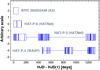 |
Fig. 1 Time distribution of the secondary datasets used in combination with the mock TESS data to test search methods for periodic transit signals detected as single events in the TESS data. Each block represents a continuous dataset with gaps shorterthan one day. The data are plotted relative to the time at the first observation, HJD (1). The HATnet and WASP data on HAT-P-2 are merged in signal H2 (see Table 1) for the tests presented in this paper. |
2.2 Transit signals
The basic parameters of the transit signals used in this work are given in Table 1. We focused mostly on systems with Sun-like hosts and Neptune-like planets. To test single-transit events down to ~ 15 days, we fixed the center of the transit in the middle of the time span of the primary set T0. The three types of signal represent various signal–noise settings: type a for shallow signals in the presence of low noise, type b for shallow signals in the presence of medium to high noise, and type c for signals extending to the hot-Jupiter regime in the presence of medium to high noise.
We chose 100 days for the upper limit of the period to be searched for because this is about the extent of an observational season on a given field for the ground-based surveys. Furthermore, at an orbital period of 100 days for a planet around a Sun-like star, we expect a transit duration of 0.36 days, that is, far longer than the length of an average observation night. Although this difficulty can be overcome by even a modest longitudinal spread of a network of telescopes (e.g., HATNet), the problem of systematics filtering still remains for long events, comparable with the characteristic length of the continuous nightly data segments. In spite of all these difficulties, we note that ground-based surveys have already been successful in discovering systems with orbital periods longer than 10 days. For instance, HATS-17b has an orbital period of 16.25 days, with a transit duration of 0.20 days (Brahm et al. 2016). The lower limit on the transit depths to be tested may seem overly optimistic, but we show that when combined with the single-event data from the primary (space) set, this limit is quite accessible (and even those down to 0.0005 for more extended secondary sets). Ground-based surveys have already proven their ability to reach the few-millimagnitudes limit in detecting short-periodtransits (e.g., HAT-P-11 by Bakos et al. 2010, WASP-73 by Delrez et al. 2014). Because of this low limit in the detectable transit depths aided by ground-based data, the accessible systems cover a considerable upper region of the period–transit depth diagram4. We return to this aspect in Sect. 4.
Except when indicated otherwise, for the primary dataset we fixed the standard deviation to 0.0005 for the half-hour cadence. This value is more representative for the likely error budget of TESS at ~ 11 mag (i.e., Oelkers & Stassun 2018), whereas for brighter stars, 0.0002 or even lower values may be used (e.g., Shporer et al. 2019). From our point of view, the exact value does not really matter until it is considerably (i.e., by several factors) lower than the standard deviation of the secondary dataset. For the latter, the error ranges are realistic in the bright tail of the magnitude distribution (e.g., between 9 and 11 mag) for all signal types listed in Table 1; see Bakos et al. (2009). For signal type a, the errors are realistic only if the data are averaged on a 30 min cadence (i.e., for set H0).
In most of our tests we used 500 random realizations for each test case. In these realizations we chose the transit parameter δ and the standard deviation σH of the white-noise component of the signal from a uniform distribution. The same type of distribution was used for the orbital period, but this time, for a better sampling of the shorter period regime, on the logarithmic values of the period. The transit length was computed for each test period by assuming a central transit, a circular orbit, and a solar-type host (e.g., Winn 2014). The distribution of the noise component was Gaussian, with the standard deviation chosen above. We stress that these random simulations are not intended to model the observed extrasolar planet population. Instead, our purpose is solely to visit a wide but still plausible parameter space.
Last but not least, as listed in Table 1, in the actual joint analysis with the already existing ground-based data, we expect rather large gaps between these and the TESS data. This is a serious problem both from the point of the practical implementation of the signal search (the required number of test frequencies might easily exceed 105 –106 over the frequency band of ~ 0.1 d−1) and it is also bad for the signal-to-noise ratio (S/N) and thereby for the reliability of the signal search. To show the effect of a single gap of 8 yr between sets H0 and T0, we compare in Fig. 2 the resulting box-fitting least-squares (BLS) spectrum (Kovacs et al. 2002) with the spectrum obtained in the case of continuous data distribution. Although the main peak preserves the overall width of the line profile, there are subtle differences, in addition to the appearance of a forest of peaks at a lower power. When combined with noise, these aliasing effects lead to lower S/Ns, and ultimately to a lower discovery rate for data that are separated by longer gaps. Because of the practical importance of this effect, we also tested how gaps influence the results that are obtained by the optimized joint analysis presented in this paper.
Summary of the generic datasets.
2.3 BLS spectrum characterization and detection criteria
Because the method presented here is based on the optimization of the BLS frequency spectra, we here briefly summarize some of the technical details in the computation of the spectra and the parameters used to characterize the detection and signal significances. On the basis of these parameters we also define the detection criteria to be used throughout the paper to classify the various signal search methods.
For the basic tests, all frequency spectra were computed in the [νmin, 0.15] d−1 range, where νmin = 1∕Tspan, and Tspan is the total time span of the analyzed data5. For frequency sampling, in the course of extensive parameter survey, we used four samples for each central line width CLW ~ qtran∕Tspan, where qtran = t14∕Porb is the relative transit length (the ratio of the full transit duration t14 to the orbital period Porb). This sampling has a coverage of about eight spectral points throughout the full central part of the line profile (see Fig. 3).
The S/N of the frequency spectrum, S/Nsp, always referred to a given frequency band, is naturally defined as
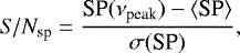 (1)
(1)
where SP(νpeak) is the value of the BLS power at the peak frequency νpeak, ⟨SP ⟩ is the average power, and σ(SP) is the standard deviation in the given frequency band. These quantities are derived from the BLS spectra after subtracting a best-fitting six th-order polynomial from the original spectra and normalizing it to [min, max] = [0, 1]. The polynomial fit is necessary to eliminate the common overall power increase at low frequency in the BLS spectra. Therefore, we employed an iterative fitting that discards outliers, that is, high peaks, at the 3σ level.
It might be a matter of dispute how to derive ⟨SP⟩ and σ(SP) because in the case of gapped data, aliasing produces additional peaks that might increase both the average and the standard deviation of the spectrum. However, periodic signals have asymptotically discrete spectra also when the data are gapped, and the straightforward computation of ⟨SP⟩ and σ(SP) could also be sufficient because the peaks still occupy only a small fraction of the frequency band investigated if this band is wide enough. Therefore, we decided not to use outlier clipping when we computed ⟨SP ⟩ and σ(SP).
In addition to the spectrum S/N, we might be interested also in the significance of the signal in the folded light curve (LC) and ask whether any conclusion might be derived from the quality of the folded LC of some hypothetical signal on the detectability of this signal in the BLS spectrum. Following Kovacs & Kovacs (2019), we considered the immediate neighborhood of the transit with the same length of out-of-transit section as the transit itself. When we assume a uniform data distribution with Nin intransit, δ transit depth and point-by-point errors with astandard deviation σ, the significance of the transit is parameterized simply by the ratio of the transit depth and the error of the difference between the averages of the in- and out-of-transit parts, i.e.,
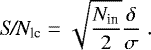 (2)
(2)
To quantify the power of the various detection methods, we need to define the criteria of detection. Since we investigate test signals with known parameters, we can easily define these conditions as follows:
- a)
The S/N of the highest peak in the frequency spectrum, S/Nsp, must be greater than S/Nmin, the lower detection limit, set according to the acceptable tolerance on the false-alarm rate (FAR): the rate of those spectra that satisfy the condition on S/Nsp, but do not satisfy the frequency condition below.
- b)
The frequency at the highest peak, νpeak, should satisfy the following condition: |νpeak − rνtest| < 2 ×CLW, where r = n∕m, with small integers to allow traceable frequency confusion, and CLW ~ qtran∕Tspan, as already defined earlier.
Including the test frequency, we check altogether 15 frequencies of the type above (i.e., we do not include alias components due to sampling). Interestingly, we find that in the large majority of cases, it is the basic frequency that comes out as the largest peak in the spectra. In the case of real data, of course, we do not know FAR for any given S/Nmin. Usually, as a rule of thumb, by taking S∕Nmin ~ 6–8 will result “meaningful” FAR values, i.e., less than ~20%. To get a more accurate estimate on FAR when real data are analyzed, one can perform an injected signal test. This will certainly increase the execution time, but supplies an important piece of information on the reliability of the suspected detection. Furthermore, a deeper examination of the spectra (e.g., alias search, including all peaks, not only the highest one) would certainly increase the detection rate by some – foreseeably small – amount. We opted not to dwell so deeply in the analysis of the frequency spectra, because the expected gain is small, and we are interested in relative detection rates, and then employing the same detection method is more important than getting a little gain by a deeper spectrum analysis. We return to the issue of detection rate and detection thresholds in Sect. 3.
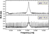 |
Fig. 2 Comparison of the BLS spectra obtained without (upper panel) or with a single 8 yr gap between the ground-based and TESS data. We use the datasets H0 and T0 (emulating the TESS data) of Table 1 with a noiseless signal of P = 35.3 days and a relative transit duration t14∕P = 0.008. Each spectrum is normalized to the respective highest peak. |
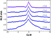 |
Fig. 3 Evolution of the line profile of the BLS frequency spectrum as a function of the gap length (ΔT (yr)) between two sets of time series (H0 and T0 of Table 1). The same signal is used as in Fig. 2. Four samples for each CLW (see text) are used (blue points). For comparison, the densely sampled profile is also shown by the pink continuous line. All profiles are normalized by the peak power and shifted vertically for better visibility. The apparent lift of the profile wings for higher ΔT values is due to the CLW units used on the abscissa. |
2.4 Optimizing S/Nsp for the joint BLS spectrum
With the far better quality of the TESS data (represented by set T0 in Table 1), it is obvious that traditional inverse variance weighting in the least-squares transit search of the joint data would not work with single-event TESS data. Therefore, we propose to search for an optimum weighting with the aid of simple scanning a range of weights, and search for the weight that yields the highest S/N for the corresponding BLS frequency spectrum. In the following we describe the basic ingredients on which our detection analysis is based, and present some examples exhibiting the characteristics of these ingredients.
First, we introduce a single parameter α that was used to weight set T0. For simplicity, we used equal weights on the data associated with the same source, that is, use α for set T0 and 1 − α for sets H#. These weights can be employed directly in the formulae of Kovacs et al. (2002) to compute the BLS spectra because these formulae allow arbitrary weighting of the data. Then we may consider various possibilities to perform the BLS analysis. In a basic setting we ignore the fact that T0 consists of data of considerably higher accuracy than H#, and with a properly chosen α, we performed atraditional BLS analysis by letting all transit parameters free to vary (but least-squares optimized) at each test period. We call this approach BLS0.
Then, following in part Yao et al. (2019), we derived the time of the transit center Tc and duration t14 from T0, and then scanned only the period to find the one that fits the full dataset. The scanning was performed within the framework of weighted BLS, whereby the transit depth is optimized at each trial period. We flagged the resulting spectrum as BLS1. An alternative approach would be try to fix the transit depth and scan only the period.6 This approach is labeled BLS2.
Before proceeding to the fourth method, we show an example of the methods introduced so far in Fig. 4. The standard BLS method with weights (uppermost panel) is able to detect the signal with a reasonable significance. This can be compared with BLS1, where the signal is apparently less significant. However, a deeper examination of the plots reveal that the noise baseline (average noise level) is higher for BLS0. Because this parameter also plays role in the calculation of S/Nsp (see Eq. (1)), the situation is more complex than it may seem at first sight. Nevertheless, it is also quite clear that the two types ofspectra display relatively little correlation in the noise-dominated frequency regime. This prompted us to attempt to improve the method and take the weighted average of the two spectra, leading to BLS3, with the corresponding spectra defined as
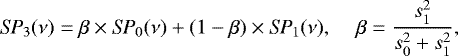 (3)
(3)
where SP0,1,3(ν) and s0,1 are the spectra and the standard deviations, respectively, corresponding to the methods described above (as indicated by the subscripts). We note that the spectra are normalized to [min,max]=[0,1] and s0,1 refer to these spectra. The BLS1 spectrum is optimized separately. The weight for BLS1 is always close to a low value, and the S/Nsp dependence on α is rather weak (see below), therefore we fixed α for BLS1. The bottom panel of Fig. 4 clearly shows the positive effect of the averaging and indicates that this method is probably preferred over the other alternatives discussed above for joint signal analysis.
We return to BLS2. It is interesting to realize that fixing all transit parameters except for the period leads to a very high sensitivity to noise and disqualifies BLS2 as a powerful method in detecting faint signals. We note that we rejected BLS2 for generic reasons, whereas Yao et al. (2019) rejected it based on the possible difficulties of combining different data from telescopes of considerably different optical properties. It is also observable that although the signal is detected with a low significance in the immediate neighborhood of the true frequency, this is spoiled by the increasing noise at higher frequencies. To understand this unexpected behavior, we examine the statistical properties of the BLS2 spectra under certain idealized conditions in Sect. 2.5. For easier reference, we briefly summarize the main ingredients of each method in Table 2.
For the maximization of S/Nsp for BLS0 and BLS1, it is important to examine whether any prediction can be made about the associated weights from the bulk statistical properties of the constituting time series. Based on a specific time series, Figs. 5 and 6 show examples of the behavior observed in most of the tests we performed. The two figures are meant to illustrate the different dependence of S/Nsp on α in the low- and high-amplitude regimes (shown in Figs. 5 and 6, respectively). The following general properties emerge from inspecting these two figures:
-
S/Nsp has a strong dependence on α for BLS0, especially for weaker signals;
-
the maximum of S/Nsp for BLS0shifts to lower α for stronger signals;
-
BLS1 has nearly flat maximum S/Nsp in the [0, 0.2] regime, independently of the strength of the signal;
-
BLS2 has nearly flat maximum S/Nsp in a very wide regime in [0, 0.8];
-
S/Nsp for BLS3 is flatter than BLS0, but has very similar properties;
-
BLS3 has the highest maximum S/Nsp among the tested methods.
Of the listed properties, the overall shift of α toward lower values for higher-quality secondary datasets seems fairly robust because it is also detected in the more extensive tests made on datasets H1+T0 and H0+T0. Figure 7 shows the resulting distributions for α from the 500 simulations for both data settings, using the same realizations (which means that the only difference between the two cases is the data distribution: H0 is continuous, H1 is gapped, but contains more data points). Because of the aliasing, the detection rate in H1 alone (dr-h1) is lower than in set H0. Therefore the effect on the optimum α is similar to the case of a lower signal amplitude, as shown in Figs. 5 and 6.
Except for the properties above, we were unable to derive any simple rule to determine α for BLS0/BLS3 and avoid the somewhat time-consuming search for the optimum value of this parameter. However, for BLS1 we can safely fix α at ~0.1 for a wide regime of data and signal parameters.
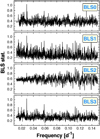 |
Fig. 4 Typical spectra obtained by variants of BLS applied on set H0+T0 of Table 1. The transit parameters are Porb = 35.12345 d, δ = 0.003, q = 0.005, σH0 = 0.002, and σT0 = 0.0005. There is no gap between H0 and T0. Economic plotting is employed using 2000 frequency bins and plotting only the maxima in each bin. Increasing the number of fixed transit parameters (from the “all free” case of BLS0 to the “all fixed” case of BLS2) decreases the detection efficacy in this faint signal regime. However, the proposed optimum combination of BLS0 and BLS1 to BLS3 significantly increases the reliability of the detection. |
Summary of the variants of the BLS routine.
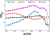 |
Fig. 5 Signal-to-noise ratio of the highest peak of the BLS spectra vs. data weight factor α for a realization of a faint transit signal on the set H0+T0 with zero gap. The transit parameters are as follows: Porb = 15.2345 d, δ = 0.003, q = 0.010, σH0 = 0.004, σT0 = 0.0005. All peak frequencies match the orbital frequency, except the very few shown by smaller symbols. See Table 2 and associated text for the definition of the various BLS methods. |
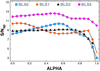 |
Fig. 6 As in Fig. 5, but for a stronger signal where all parameters are the same, except for the increased transit depth of δ = 0.005. The increased signal strength results in a shift of the optimum α toward lowervalues and some flattening of the α dependence of S/Nsp for BLS0 (and, as a result, also for BLS3). |
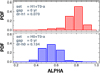 |
Fig. 7 Distribution of the optimum α values from the BLS0 analyses of datasets of different signal detection powers for the secondary sets (see Table 1). The detection ratios obtained from the BLS analyses of the secondary sets alone are given by dr-h0 and dr-h1. All data points used in the construction of the histogram satisfy the detection criteria with S∕Nmin = 6. We use the same 500 realizations in both datasets. Aliasing in set H1 boosts α to higher values for optimized BLS0 performance. |
2.5 Statistical properties of BLS2
We assumedthat (i) the secondary dataset contains only a single transit, and (ii) only those trial periods are tested that generate transits that either have full overlap or no overlap at all with the true transit in the secondary dataset. The time series of the secondary set has the form of x(i) = T(i) + ξ(i), where T(i) = δ, if i1 < i < i2, and zero for all the other n data points of {x}. The noise component {ξ} is assumed to be Gaussian and white, i.e., the following relations are held for the expectation values: < ξ>= 0, < ξ2 >= σ2, < ξ3 >= 0, < ξ4 >= 3σ4 and < ξ(i)ξ(j) >= 0 for any i≠ j. When the correct signal frequency ν0 is hit, the average squared deviation of the residuals is computed by
 (4)
(4)
For test periods that do not yield overlap with the single event in the secondary dataset, there are k trial transits in the out-of-transit part of the data, and there is an out-of-transit part of the trial signal at the transit section of the data. Assuming that all transits include the same number of m data points, we have
 (5)
(5)
where {η} is some subset of the full set of {ξ} and disjunct from the set entering in the first sum. The first two moments of D(ν0) and D(ν) can easily be derived from the above expressions and the statistical properties of {ξ}. We find
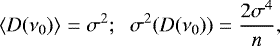 (6)
(6)
 (7)
(7)
where  . As expected, the spectra show an overall linear increase in the average power toward higher frequencies. In principle, this would not be a problem because the spectra are filtered out from polynomial trends. However, the similar increase in frequency-dependent variance degrades the result. When we normalize the variance of the spectrum to the value at the true frequency, we obtain for the relative increase of the variance
  , which confirmes what we see in the actual numerical tests (see Fig. 4).
3 Efficacy of the joint analysis
Before we investigate the power of the joint analysis, we briefly discuss the basic patterns of the detection rates and FARs that are the basic parameters for comparing the power of the various detection methods. We define two types of detection rate: (i) the observed rate DRobs, where the only requirement is to satisfy the  criterion, and (ii) the true rate DRtrue, satisfying both the above and the frequency match criteria (see Sect. 2.3). We denote the number of cases that satisfy condition (i) by NS/N, and those that also satisfy the frequency condition by NS/N,ν. We recall that the FAR is then simply FAR = 1.0 − NS/N,ν∕NS/N. It follows then that DRtrue = (1 −FAR) ×DRobs.
Figure 8 shows the variation of these rates as a function of  . For the particular dataset we tested, FAR drops quickly near zero for
  in [5,7] and increasing number of the frequencies at highest peaks come into agreement with the injected signal frequencies. Unfortunately, the convergence interval could be shifted to other values of
  if the total time span is not covered uniformly, for instance, unlike in the case shown in Fig. 8. Aliasing increases the number of high peaks, thereby decreasing the chance of hitting the correct frequency at the highest peak. This situation is illustrated in Fig. 9, where except for the gap between the two datasets, the same sets and signals are used as above7.
In spite of the higher FAR for the gapped data in the standard S/N regime, we caution (again) that our simple criteria for frequency identification lack deeper examination of the spectra. It may be that a more sophisticated peak statistics that also includes alias components would reveal somewhat better detection rates even in the case of gapped datasets.
In the following we test the detection capability of the three methods suggested in Sect. 2.4. To compare the effect of gaps both between the primary and the secondary sets, and those in the secondary set alone, we used sets H0+T0 and H1+T0 with and without a 1 yr gap betweenthe primary and secondary sets. Figure 10 shows the variation in detection rates as a function of the S/Nsp cutoff. The important common feature in both the gapped and non-gapped cases is the same hierarchy of the three methods. BLS3 outperforms the other two methods throughout the signal-dominated regime (e.g., for  5.5).
5.5).
The somewhat more realistic setting, with the secondary set H1 (where the sampling is interrupted by daily and longer gaps) Fig. 11 shows that the properties mentioned above are retained, with some modification in the actual statistics. Although BLS3 still outperforms BLS1, the difference becomes less significant. The detection rates increase because of the larger data volumepossessed by H1 (which apparently wins over the gaps within the dataset, which work against the higher detection rate). Compared with the FAR displayed in Fig. 10, we observe a lower decline, also attributed to the gapped nature of the secondary set.
Because the detection rates result from random simulation, it is a valid concern whether the number of realizations (i.e., 500 in our tests) is enough for drawing reliable conclusions from these simulations. We note that these simulations are meant to cover a relatively large parameter space consisting ofPorb, δ, and σ, and for each given set of parameters, the time series generated by the particular noise realization. Therefore, we performed additional tests, with different seeds for the random number generator, to show how the detection rates change. For simplicity, we chose H0+T0 with signal type a and zero gap. For compatibility with the basic tests, we used 500 realizations. The result is displayed in Fig. 12. It is clear that there is some dependence on the realization, but the relative relation of the different search methods still remain essentially the same, that is, the order of preference of the different methods does not change (neither qualitatively nor quantitatively).
Next we addressed the natural question whether the traces of the signal can be detected even in the secondary dataset without using any information from the primary set. If so, then what percentage of them are reliable detections? We chose two examples to illustrate the remarkable signal-boosting capability of the high-S/N single transit in the primary dataset T0.
In Fig. 13 we plot the ratio of the spectrum S/N values for the “H0 alone” and “H0+T0” cases as a function of S/Nsp for BLS3. In an overwhelming majority of cases, the signals would have remained undetected in the standard BLS analysis of the secondary set H0 alone. In the 500 realizations of signal type a, the BLS3 analysis discovers 37% of them. This can be compared with the 7% success rate from analyzing H0 alone.
Yet another way of considering the detection rate increase by the joint analysis is to check if in any given case the strength of the signal implies detection, and if so, whether it is detected in the secondary set. Unfortunately, there is no parameter that would be based solely on the significance of the signal in the folded light curve and would predict detectability. The reason for this is that the folded light curve lacks basic information on other signal components such as noise with semi-periodic components or real signals. Nevertheless, S/Nlc (see Eq. (2)), computed from the signal parameters as realized in H1, might still have some relevance, and we tested its capability here.
First of all, we note that we were able to perform this test in the present case because the signal parameters were known from the simulations. For real data, S/Nlc can only be estimated probabilistically because the number of in-transit data points is not known because it is the function of the period (which is not known either).
We found that the result of this test is quite similar for all signal types discussed in this paper. One example is shown in Fig. 14 for signal type c (the case when most of the signals are strong, but so is the ambient noise). The joint analysis amplifies the true signal content not only for stronger signals of S∕Nlc > 5, but even for very faint signals with S∕Nlc < 3. The detections in the “H1 alone” analyses remain mostly in the low S/Nsp regime, depending only mildly on S/Nlc. Consequently, the detection rate for BLS3 on H1+T0 is much higher, exceeding the rate of the “H1 alone” analysis by several factors. For instance, with S∕Nmin = 6.0, we find observed rates of 0.83 and 0.09 with respective FARs of 0.12 and 0.16.
It is interesting to examine how the behavior of the weight factor α changes when multiple transit events are observable in the TESS (T0) data. It is expected that the optimum weight switches back to the standard inverse-variance weighting that leads to the minimum variance of the combined dataset. To check this inference, we used the H0+T0 set with zero gap between H0 and T0. Except for the phase, we fixed all signal parameters, namely P = 22.3 d, δ = 0.002, σH0 = 0.003, and used BLS0 on ten random realizations. By shifting the signal in phase, we can control the number of transit events occurring in set T0.
Figure 15 shows that in the single-transit regime, the optimum α is relatively constant around the value of 0.75. In the two-transit regime (i.e., outside the gray shaded box), α is mildly bimodal. Most of the values are very close to 1.0, as expected from the inverse-variance weighting, predicting α = 0.0032∕(0.0032 + 0.00052) = 0.97. In some cases the optimum single-transit values are preferred. A closer examination of the run of S/Nsp(α) shows that this function tends to be double-humped, and depending on the phase, noise realization, and data distribution, the lower α values are preferred in rare cases even when multiple transits are available from the primary dataset T0. For comparison, we also show the relative frequency distance 1 − νT0∕νtest for the peak frequency of the spectrum of T0. The signal is detectable in the two-transit regime, and as expected, cannot be recovered in the single-transit regime.
To further assess the signal detection capability of the joint analysis of the space- and ground-based data, we tested the dataset H2+T0, with H2 spanning over three years and containing some forty-five thousand data points (see Table 1). Our test was very limited: (a) we assumed that this dataset was placed immediatelybefore the TESS data, that is, there is no gap between them. (b) We fixed the period to two values, P = 17.3 d to test the short-period regime with transit phase allowing only a single transit in the TESS data, and P = 25.3 d to test the longer period, close to the regime when only single transits are possible. (c) The noise was fixed for H2 to σH2 = 0.003 and for T0 to σT0 = 0.0002. (d) The weight factor was set to α = 0.97, based on few detailed runs for the optimization of this parameter. (e) The transit depth was scanned in four values: (0.02, 0.04, 0.06, 0.08)%. (f) For each transit depth, we ran 100 random simulations to gain some information on the effect of noise realization. The transit duration was computed in the same way as in the case of the basic simulations discussed earlier (see Table 1). Although these simulations are by no means meant to fully characterize the detection capability of H2 with T0, they give at least some indication on the accessible planet population in an almost ideal case.
The detection rates and some accompanying quantities for these simulations are displayed in Table 3. The lower detection rates for the longer period case are attributed to the lower number of in-transit data points (294 vs. 587 in the short-period simulations). Nevertheless, the sub-ppt regime down to ~ 0.5 ppt, although with substantially increased FARs, are accessible in both cases. While for higher S/Ns at δ = 0.6 ppt the ratio of the joint versus “H2 alone” detection rates is only 4 in the short period case, this increases to 30 at δ = 0.4 ppt. Shifted to larger transit depths, the situation is similar for the longer period case.
To illustrate the signal detection power of the joint analysis in a “twilight zone” (i.e., at the verge of detection) case, Figs. 16 and 17 show the time series and the frequency spectra, respectively. For comparison, in the upper two panels of Fig. 17 the spectra of the separate analyses of H2 and T0 are also shown.
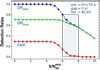 |
Fig. 8 Dependence of the detection rate on the lower limit of the spectrum S/N. The observed rates DRobs are calculated solely on the basis of satisfying the S∕N > S∕Nmin criterion and do not consider the match of the peak frequency to the test frequency. The true detection rate DRtrue results from the correction of the observed rate by the FAR, namely, DRtrue = (1 −FAR) ×DRobs. The signal identification and analysis method are indicated in the upper right corner. The most commonly used range for the lower limit of the spectrum S/N is shown by the gray rectangle. We use 500 random realizations of the signal shown in the header; see also Table 1. |
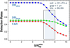 |
Fig. 9 As in Fig. 8, but for the simulations with 1 yr gap between the primary and secondary datasets. Aliasing leads to higher FARs and concomitant lower true detection rates in the S/N regime that is best for continuously sampled data. |
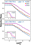 |
Fig. 10 True detection rates for dataset H0+T0-a using various signal search methods (BLS0, BLS1, and BLS3 with respective detection rates of DR0, DR1, and DR3). Upper and lower panels: results obtained with zero and 1 yr gap between H0 and T0. The FARs used to correct the observed detection rates are displayed in the insets. For gapped data, the FAR increases considerably, leading to a decrease in the true detection rates. |
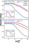 |
Fig. 11 As in Fig. 10, but for set H1+T0. We observe a similar pattern as for H0+T0, with competing effects of the gapped nature of H1 and the substantial increase in the size of data for the same dataset. |
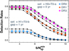 |
Fig. 12 Testing the effect of the noise realization. Dots colored other than black denote our standard random number initialization. Smaller black dots show the results obtained with different seeds for the random number generator. Upper and lower lines for these tests for each standard simulation resulted from the same pair of seeds. Labels have the same meaning as in Fig. 10. |
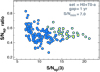 |
Fig. 13 Comparison of the number of detections from the joint analysis by BLS3 (blue points) with those resulting from the standard BLS analysis of the secondary dataset H0 alone (yellow points). Spectrum S/N for the analysis by BLS3 on “H0+T0” is denoted by S/Nsp (3). The ordinate shows the ratio of the spectrum S/N values for “H0 alone” over “H0+T0”. Signal type a with 500 realizations was used. |
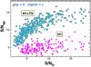 |
Fig. 14 Signal-to-noise ratios derived from phase-folded time series S/Nlc vs. those of the corresponding BLS spectra, S/Nsp, for simulations satisfying the frequency criterion, condition b in Sect. 2.3. The joint analysis (by using BLS3) is capable of boosting even those signals that are otherwise buried deep in the noise (i.e., have S ∕Nlc < 3.0 in the “H1 alone” standard BLS analysis). |
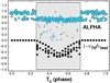 |
Fig. 15 Dependence of the weight factor α of BLS3 onthe phase of the transit center in the case of intermediate periods, when two transits may be observed in the TESS data (T0) alone. The single-transit phase interval is indicated by the gray shaded box. The optimum α values are shown by the overlapping blue points (smaller dots mean no detection from the ten realizations we tested). We added a small noise to each point resulting from the grid scan to highlight the population density. Black dots indicate the relative peak frequency values for the primary dataset T0, indicating detection in the two-transit regime, and lack of it in the single-transit regime. See text for additional details. |
Extended dataset (H2+T0) detection rates.
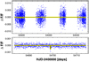 |
Fig. 16 Simulated time series exhibiting the overall characteristics of the signals generated on the time distribution of sets H2 and T0 (upper and lower panels, respectively). The synthetic signal is shown by the black continuous line (in a yellow silhouette for better visibility). The signal parameters are P = 17.3 d, δ = 0.0005, t14∕P = 0.011, σT0 = 0.0002, and σH2 = 0.003 (see also Table 1). Only every tenth data point is plotted for H2 for clarity. |
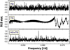 |
Fig. 17 Frequency spectra of the time series shown in Fig. 16. We use α = 0.97 in the computation of the BLS3 spectrum of the combined dataset. The signal is not detected in the “H2 alone” analysis (for T0 the detection is ab initio excluded due to the lack of multiple transit events). |
4 Conclusions
A combination of ground- and space-based observations is usually complimentary because of the different precision, wavelength, resolution, time span, etc. There are also ultraprecise data (i.e., those gathered by the Kepler satellite) that remain in the realm ofspace observatories. Nevertheless, even in these cases, ground-based data might be extremely useful when the signal is not hopelessly below the detection limit of the ground-based instruments. We investigated a case that falls in this category: a scenario when only a single transit is observed from space. We showed that an optimum combination of these and the ground-based data leads to a secure transit signal detection, allowing full photometriccharacterization of the system, including the period. The main steps of the suggested method are listed below.
Step0: determining the transit parameters Tc (transit center) and t14 (transit duration) from the space data →
Step1: transit search with these parameters fixed and the ground-based data heavily weighted →
Step2: repeating the search with free-floating transit parameters, a standard BLS search with fixed weights: α for the space- and 1 − α for the ground-based data
Step3: inverse-variance averaging of the normalized frequency spectra of Step1 and Step2 →
Step4: repeat Step2 by scanning the weight α to find its optimum value by maximizing the S/Ns of the average spectra.
We found that the optimum weight on the ground-based data in Step1 is between 0.9 and 1.0 in almost all cases. To save execution time, we can therefore fix this weight in this interval. On the other hand, weight α is a more complicated function of the actual data and signal settings. Nevertheless, we found that it is always greater than 0.5. Therefore, this parameter should be scanned in [0.5, 1.0] and its optimum value be determined according to Step4. Depending on the grid on α, all these steps lead to a multifold increase in the execution time. In a preliminary survey of the data, Step0 and Step1 may already be enough, because the spectrum derived in Step1 might have sufficient S/N to identify the period. However, as discussed in this paper, the spectra obtained after performing full optimization (Step3) will certainly be of higher quality, and thereby lead to detections of higher confidence. In crucial cases of low S/N, the full four-step procedure above may be the only way to determine the correct period.
The detection power of the optimum-weighted joint analysis surpasses that of an analysis that is based on ground-based data alone by a factor of 2–10. Consequently, no detection in an analysis based on ground-based data alone does not mean that these data are not useful. Naturally, the generic problem of a period search in gapped data also holds in this case: larger gaps make the detection less likely because of the increased complexity of the frequency spectrum. Therefore, continuation of the ground-based surveys even under running precise space-based surveys is strongly preferred, as compared to relying only on data gathered several years ago. Naturally, both to decrease the noise level and to increase the duty cycle, a combination of various ground-based survey data is very useful.
As indicated in Sect. 3, even under ideal circumstances, the combination of ground- and space-based surveys is unlikely to discover transits shallower than ~0.03% (see Table 3). Even so, this is a very remarkable lower limit that enables us to sample the Neptune – sub-Neptune population quite deeply. Figure 18 shows the region that is expected to be covered by the joint analysis of the space- and ground-based data in the orbital period–transit depth plane. We used the NASA Exoplanet Archive8 to show the currently known population of confirmed transiting extrasolar planets. The lower limits on the transit depth are highlighted in green and fuchsia. These limits are based on the simulations presented in this paper, supplemented by some additional simulations on dataset H2 of Table 1.
The regime of the jointly discovered planets is expected to be confined mostly to the relatively sparsely populated part of this diagram. It would be important to sample this part more effectively because these systems will be important in the near future, when lower temperature gas giants (more similar to our Neptune) will be the targets of atmospheric characterization.
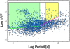 |
Fig. 18 Accessible transiting extrasolar planets for TESS single-sector observations (shaded regions) in the period–transit depth diagram. The green shaded polygon covers the region where the data from TESS alone are enough for the detection. The yellow shaded region shows where ground-based data are required, whereas in the hatched intermediate region, a proper transit phase might make the detection possible using the TESS data alone. Dots denote the confirmed transiting extrasolar planets according to the NASA Exoplanet Archive. See text for details on the detection limits. |
Acknowledgements
It is a pleasure to thank the referee for the constructive comments. Support from the National Research, Development and Innovation Office (grants K 129249 and NN 129075) is acknowledged.
References
- Bakos, G., Noyes, R. W., Kovács, G., et al. 2004, PASP, 116, 266 [NASA ADS] [CrossRef] [Google Scholar]
- Bakos, G. Á., Kovács, G., Torres, G., et al. 2007, ApJ, 670, 826 [NASA ADS] [CrossRef] [Google Scholar]
- Bakos, G. Á., Noyes, R. W., Kovács, G., et al. 2009, IAU Symp., 253, 21 [NASA ADS] [Google Scholar]
- Bakos, G. Á., Torres, G., Pál, A., et al. 2010, ApJ, 710, 1724 [NASA ADS] [CrossRef] [Google Scholar]
- Barclay, T., Pepper, J., Quintana, E. V. 2018, ApJS, 239, 2 [NASA ADS] [CrossRef] [Google Scholar]
- Becker, J. C., Vanderburg, A., Rodriguez, J. E., et al. 2019, AJ, 157, 19 [NASA ADS] [CrossRef] [Google Scholar]
- Bouma, L. G., Winn, J. N., Kosiarek, J., & McCullough, P. R. 2017, ArXiv e-prints [arXiv:1705.08891] [Google Scholar]
- Brahm, R., Jordán, A., Bakos, G. Á., et al. 2016, AJ, 151, 89 [NASA ADS] [CrossRef] [Google Scholar]
- Cooke, B. F., Pollacco, D., West, R., et al. 2018, A&A, 619, A175 [NASA ADS] [CrossRef] [EDP Sciences] [Google Scholar]
- Delrez, L., Van Grootel, V., Anderson, D. R., et al. 2014, A&A, 563, A143 [NASA ADS] [CrossRef] [EDP Sciences] [Google Scholar]
- Dzigan, Y., & Zucker, S. 2011, MNRAS, 415, 2513 [NASA ADS] [CrossRef] [Google Scholar]
- Dzigan, Y., & Zucker, S. 2013, MNRAS, 428, 3641 [NASA ADS] [CrossRef] [Google Scholar]
- Foreman-Mackey, D., Montet, B. T., Hogg, D. W., et al. 2015, ApJ, 806, 215 [NASA ADS] [CrossRef] [Google Scholar]
- Huang, C. X., Shporer, A., Dragomir, D., et al. 2018, AJ, submitted [arXiv:1807.11129v1] [Google Scholar]
- Kipping, D. 2018, Res. Notes AAS, 2, 4 [Google Scholar]
- Kovacs, G., & Kovacs, T. 2019, A&A, 625, A80 [NASA ADS] [CrossRef] [EDP Sciences] [Google Scholar]
- Kovács, G., Zucker, S., & Mazeh, T. 2002, A&A, 391, 369 [NASA ADS] [CrossRef] [EDP Sciences] [Google Scholar]
- Noyes, R. W., Bakos, G. Á., Torres, G., et al. 2008, ApJ, 673, L79 [NASA ADS] [CrossRef] [Google Scholar]
- Oelkers, R. J., & Stassun, K. G. 2018, AJ, 156, 132 [NASA ADS] [CrossRef] [Google Scholar]
- Osborn, H. P., Armstrong, D. J., Brown, D. J. A., et al. 2016, MNRAS, 457, 2273 [NASA ADS] [CrossRef] [Google Scholar]
- Pepper, J., Pogge, R. W., DePoy, D. L., et al. 2007, PASP, 119, 923 [NASA ADS] [CrossRef] [Google Scholar]
- Pepper, J., Kuhn, R. B., Siverd, R., et al. 2012, PASP, 124, 230 [NASA ADS] [CrossRef] [Google Scholar]
- Pollacco, D. L., Skillen, I., Collier Cameron, A., et al. 2006, PASP, 118, 1407 [NASA ADS] [CrossRef] [Google Scholar]
- Ricker, G. R., Winn, J. N., Vanderspek, R., et al. 2015, J. Astron. Telesc. Instrum. Syst., 1, 014003 [NASA ADS] [CrossRef] [Google Scholar]
- Seager, S., & Mallen-Ornelas, G. 2003, ApJ, 585, 1038 [NASA ADS] [CrossRef] [Google Scholar]
- Shporer, A., Bakos, G. Á., Mazeh, T., et al. 2009, IAU Symp., 253, 331 [NASA ADS] [Google Scholar]
- Shporer, A., Wong, I., Huang, C. X., et al. 2019, AJ, 157, 178 [NASA ADS] [CrossRef] [Google Scholar]
- Sullivan, P. W., Winn, J. N., Berta-Thompson, Z. K., et al. 2015, ApJ, 809, 77 (Erratum: 2017, ApJ, 837, 99) [NASA ADS] [CrossRef] [Google Scholar]
- Vanderburg, A., Becker, J. C., Kristiansen, M. H., et al. 2016, ApJ, 827, L10 [NASA ADS] [CrossRef] [Google Scholar]
- Villanueva, S. Jr., Dragomir, D., & Gaudi, B. S. 2019, AJ, 157, 84 [NASA ADS] [CrossRef] [Google Scholar]
- Winn, J. N. 2014, ArXiv e-prints [arXiv:1001.2010v5] [Google Scholar]
- Yao, X., Pepper, J., Gaudi, B. S., et al. 2019, AJ, 157, 37 [NASA ADS] [CrossRef] [Google Scholar]
- Yee, J. C., & Gaudi, B. S. 2008, ApJ, 688, 616 [NASA ADS] [CrossRef] [Google Scholar]
We rounded the nominal length of 27.4 days of the single-sector coverage and omitted the relatively short gap of 16 h for pointing and data download at perigee (see Ricker et al. 2015, and to illustrate the quality of the TESS data, the full phase curve of WASP-18 by Shporer et al. 2019).
This was also mentioned in Yao et al. (2019), but was discarded as an improper approach because of the complications that might arise from the different quality of the KELT and TESS images. We also discarded this method, but for a different reason (see Sect. 2.5).
To be more specific, we use the same random numbers to generate the noise and signal parameters. However, because of the gap between H0 and T0, and because of the fixed position of the transit in T0, the same signal is shifted in time in H0 in respect to its original epoch in the case of continuous data sampling.
See https://exoplanetarchive.ipac.caltech.edu/ as of 2019-02-09.
All Tables
All Figures
|
Fig. 1 Time distribution of the secondary datasets used in combination with the mock TESS data to test search methods for periodic transit signals detected as single events in the TESS data. Each block represents a continuous dataset with gaps shorterthan one day. The data are plotted relative to the time at the first observation, HJD (1). The HATnet and WASP data on HAT-P-2 are merged in signal H2 (see Table 1) for the tests presented in this paper. |
| In the text | |
|
Fig. 2 Comparison of the BLS spectra obtained without (upper panel) or with a single 8 yr gap between the ground-based and TESS data. We use the datasets H0 and T0 (emulating the TESS data) of Table 1 with a noiseless signal of P = 35.3 days and a relative transit duration t14∕P = 0.008. Each spectrum is normalized to the respective highest peak. |
| In the text | |
|
Fig. 3 Evolution of the line profile of the BLS frequency spectrum as a function of the gap length (ΔT (yr)) between two sets of time series (H0 and T0 of Table 1). The same signal is used as in Fig. 2. Four samples for each CLW (see text) are used (blue points). For comparison, the densely sampled profile is also shown by the pink continuous line. All profiles are normalized by the peak power and shifted vertically for better visibility. The apparent lift of the profile wings for higher ΔT values is due to the CLW units used on the abscissa. |
| In the text | |
|
Fig. 4 Typical spectra obtained by variants of BLS applied on set H0+T0 of Table 1. The transit parameters are Porb = 35.12345 d, δ = 0.003, q = 0.005, σH0 = 0.002, and σT0 = 0.0005. There is no gap between H0 and T0. Economic plotting is employed using 2000 frequency bins and plotting only the maxima in each bin. Increasing the number of fixed transit parameters (from the “all free” case of BLS0 to the “all fixed” case of BLS2) decreases the detection efficacy in this faint signal regime. However, the proposed optimum combination of BLS0 and BLS1 to BLS3 significantly increases the reliability of the detection. |
| In the text | |
|
Fig. 5 Signal-to-noise ratio of the highest peak of the BLS spectra vs. data weight factor α for a realization of a faint transit signal on the set H0+T0 with zero gap. The transit parameters are as follows: Porb = 15.2345 d, δ = 0.003, q = 0.010, σH0 = 0.004, σT0 = 0.0005. All peak frequencies match the orbital frequency, except the very few shown by smaller symbols. See Table 2 and associated text for the definition of the various BLS methods. |
| In the text | |
|
Fig. 6 As in Fig. 5, but for a stronger signal where all parameters are the same, except for the increased transit depth of δ = 0.005. The increased signal strength results in a shift of the optimum α toward lowervalues and some flattening of the α dependence of S/Nsp for BLS0 (and, as a result, also for BLS3). |
| In the text | |
|
Fig. 7 Distribution of the optimum α values from the BLS0 analyses of datasets of different signal detection powers for the secondary sets (see Table 1). The detection ratios obtained from the BLS analyses of the secondary sets alone are given by dr-h0 and dr-h1. All data points used in the construction of the histogram satisfy the detection criteria with S∕Nmin = 6. We use the same 500 realizations in both datasets. Aliasing in set H1 boosts α to higher values for optimized BLS0 performance. |
| In the text | |
|
Fig. 8 Dependence of the detection rate on the lower limit of the spectrum S/N. The observed rates DRobs are calculated solely on the basis of satisfying the S∕N > S∕Nmin criterion and do not consider the match of the peak frequency to the test frequency. The true detection rate DRtrue results from the correction of the observed rate by the FAR, namely, DRtrue = (1 −FAR) ×DRobs. The signal identification and analysis method are indicated in the upper right corner. The most commonly used range for the lower limit of the spectrum S/N is shown by the gray rectangle. We use 500 random realizations of the signal shown in the header; see also Table 1. |
| In the text | |
|
Fig. 9 As in Fig. 8, but for the simulations with 1 yr gap between the primary and secondary datasets. Aliasing leads to higher FARs and concomitant lower true detection rates in the S/N regime that is best for continuously sampled data. |
| In the text | |
|
Fig. 10 True detection rates for dataset H0+T0-a using various signal search methods (BLS0, BLS1, and BLS3 with respective detection rates of DR0, DR1, and DR3). Upper and lower panels: results obtained with zero and 1 yr gap between H0 and T0. The FARs used to correct the observed detection rates are displayed in the insets. For gapped data, the FAR increases considerably, leading to a decrease in the true detection rates. |
| In the text | |
|
Fig. 11 As in Fig. 10, but for set H1+T0. We observe a similar pattern as for H0+T0, with competing effects of the gapped nature of H1 and the substantial increase in the size of data for the same dataset. |
| In the text | |
|
Fig. 12 Testing the effect of the noise realization. Dots colored other than black denote our standard random number initialization. Smaller black dots show the results obtained with different seeds for the random number generator. Upper and lower lines for these tests for each standard simulation resulted from the same pair of seeds. Labels have the same meaning as in Fig. 10. |
| In the text | |
|
Fig. 13 Comparison of the number of detections from the joint analysis by BLS3 (blue points) with those resulting from the standard BLS analysis of the secondary dataset H0 alone (yellow points). Spectrum S/N for the analysis by BLS3 on “H0+T0” is denoted by S/Nsp (3). The ordinate shows the ratio of the spectrum S/N values for “H0 alone” over “H0+T0”. Signal type a with 500 realizations was used. |
| In the text | |
|
Fig. 14 Signal-to-noise ratios derived from phase-folded time series S/Nlc vs. those of the corresponding BLS spectra, S/Nsp, for simulations satisfying the frequency criterion, condition b in Sect. 2.3. The joint analysis (by using BLS3) is capable of boosting even those signals that are otherwise buried deep in the noise (i.e., have S ∕Nlc < 3.0 in the “H1 alone” standard BLS analysis). |
| In the text | |
|
Fig. 15 Dependence of the weight factor α of BLS3 onthe phase of the transit center in the case of intermediate periods, when two transits may be observed in the TESS data (T0) alone. The single-transit phase interval is indicated by the gray shaded box. The optimum α values are shown by the overlapping blue points (smaller dots mean no detection from the ten realizations we tested). We added a small noise to each point resulting from the grid scan to highlight the population density. Black dots indicate the relative peak frequency values for the primary dataset T0, indicating detection in the two-transit regime, and lack of it in the single-transit regime. See text for additional details. |
| In the text | |
|
Fig. 16 Simulated time series exhibiting the overall characteristics of the signals generated on the time distribution of sets H2 and T0 (upper and lower panels, respectively). The synthetic signal is shown by the black continuous line (in a yellow silhouette for better visibility). The signal parameters are P = 17.3 d, δ = 0.0005, t14∕P = 0.011, σT0 = 0.0002, and σH2 = 0.003 (see also Table 1). Only every tenth data point is plotted for H2 for clarity. |
| In the text | |
|
Fig. 17 Frequency spectra of the time series shown in Fig. 16. We use α = 0.97 in the computation of the BLS3 spectrum of the combined dataset. The signal is not detected in the “H2 alone” analysis (for T0 the detection is ab initio excluded due to the lack of multiple transit events). |
| In the text | |
|
Fig. 18 Accessible transiting extrasolar planets for TESS single-sector observations (shaded regions) in the period–transit depth diagram. The green shaded polygon covers the region where the data from TESS alone are enough for the detection. The yellow shaded region shows where ground-based data are required, whereas in the hatched intermediate region, a proper transit phase might make the detection possible using the TESS data alone. Dots denote the confirmed transiting extrasolar planets according to the NASA Exoplanet Archive. See text for details on the detection limits. |
| In the text | |
Current usage metrics show cumulative count of Article Views (full-text article views including HTML views, PDF and ePub downloads, according to the available data) and Abstracts Views on Vision4Press platform.
Data correspond to usage on the plateform after 2015. The current usage metrics is available 48-96 hours after online publication and is updated daily on week days.
Initial download of the metrics may take a while.