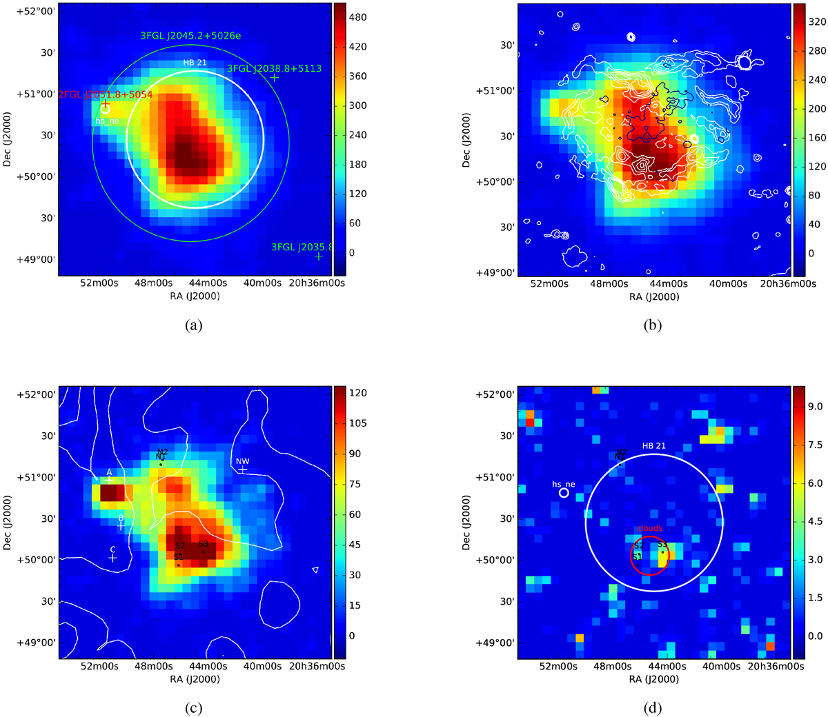
Test statistic map of the selected ROI around the SNR HB 21. The map in panel a is computed in the whole energy interval considered for the analysis, i.e., above 60 MeV. Overlaid to this map, the 3FLG sources are reported; 3FGL J2045.2+5026e is also included and defined in the catalog as a disk-type geometry with a radius of 1°.19 (green markers). The best-fit model for the SNR HB 21 as found in this work is also shown (disk-type geometry with a radius of 0°.83), together with the nearby hotspot hs_ne (white regions). The position of the point source 2FGL J2051.8+5054 is presented as well (red cross). Panel b: TS map above 500 MeV is presented, together with the contours of radio continuum emission at 4850 MHz (white) and the ROSAT X-ray (dark blue) contours. The ROSAT data are available at https://skyview.gsfc.nasa.gov/current/cgi/titlepage.pl. Panel c: for energies above 1 GeV. On top of the TS map, the CO contours are reported in white. The CO distribution are taken from Dame et al. (2001) and integrated between −20 and 10 km s⁻¹: six contour levels are linearly spaced from 1.5 to 28 K km s⁻¹. We also show the position of the shocked CO clumps S1, S2, S3, N1, N2 (black circles; Koo et al. 2001) and clouds A, B, C (Tatematsu et al. 1990) and NW (Byun et al. 2006; white crosses). Panel d: TS map of the residual emission of the best modeling of the SNR and the hotspot (white regions) is shown above 1 GeV. In addition, the position of the shocked CO clumps is reported, together with the estimated cloud region (red region).