| Issue |
A&A
Volume 621, January 2019
|
|
|---|---|---|
| Article Number | A91 | |
| Number of page(s) | 16 | |
| Section | Cosmology (including clusters of galaxies) | |
| DOI | https://doi.org/10.1051/0004-6361/201833530 | |
| Published online | 15 January 2019 | |
Multiply imaged time-varying sources behind galaxy clusters
Comparing fast radio bursts to QSOs, SNe, and GRBs
1
Universität Heidelberg, Zentrum für Astronomie, Astron. Rechen-Institut, Mönchhofstr.12–14, 69120 Heidelberg, Germany
e-mail: j.wagner@uni-heidelberg.de
2
Expertisecentrum voor Digitale Media, Universiteit Hasselt, Wetenschapspark 2, 3590 Diepenbeek, Belgium
e-mail: jori.liesenborgs@uhasselt.be
3
Department of Physics, Ben-Gurion University, PO Box 653, Beer-Sheva 84105, Israel
e-mail: eichler@bgumail.bgu.ac.il
Received:
30
May
2018
Accepted:
21
November
2018
With upcoming (continuum) surveys of high-resolution radio telescopes, detection rates of fast radio bursts (FRBs) might approach 105 per sky per day by future extremely large observatories, such as the possible extension of the Square Kilometer Array (SKA) to a phase-2 array. Depending on the redshift distribution of FRBs and using the repeating FRB121102 as a model, we calculate a detection rate of multiply imaged FRBs with their multiply imaged hosts caused by the distribution of galaxy-cluster-scale gravitational lenses of the order of 10−4 per square degree per year for a minimum total flux of the host of 10 μJy at 1.4 GHz for SKA phase 2. Our comparison of estimated detection rates for quasars (QSOs), supernovae (SNe), gamma ray bursts (GRBs), and FRBs shows that multiple images of FRBs could be more numerous than those of GRBs and SNe and as numerous as multiple images of QSOs. Time delays between the multiple images of an FRB break degeneracies in model-based and model-independent lens reconstructions as other time-varying sources do, yet without a microlensing bias, as FRBs are more point-like and have shorter duration times. We estimate the relative imprecision of FRB time-delay measurements to be 10−10 for time delays on the order of 100 days for galaxy-cluster-scale lenses, yielding more precise (local) lens properties than time delays from the other time-varying sources. Using the lens modelling software Grale, we show the increase in accuracy and precision of the reconstructed scaled surface mass density map of a simulated cluster-scale lens when adding time delays for one set of multiple images to the set of observational constraints.
Key words: dark matter / gravitational lensing: strong / methods: analytical / galaxies: clusters: general / galaxies: clusters: intracluster medium / galaxies: luminosity function / mass function
© ESO 2019
1. Introduction
Fast radio bursts (FRBs) are transients of a few milliseconds in duration. Serendipitously, 60 such bursts have been observed in the frequency ranges of about 0.4–6 GHz, Petroff et al. (2016)1. Due to the low angular resolution of continuum sky radio surveys, FRBs have only been observed in the time domain so far with best localisation precisions on the order of arcminutes. Yet, one FRB, FRB121102, showed repeating bursts, meaning that its angular position could be determined to milliarcsecond precision and the redshift of its host galaxy as z = 0.193 (Bassa et al. 2017; Chatterjee et al. 2017; Marcote et al. 2017; Tendulkar et al. 2017).
Given upcoming radio surveys with increased resolution, sky coverage, and field of view, like those made possible by the Square Kilometre Array (SKA) in phase 1 and 2, the origin and nature of FRBs can be investigated in more detail. Current investigations are detailed for instance in Dai & Lu (2017), Katz (2018), Waxman (2017). Estimated detection rates of FRBs of future sky surveys, are, for instance, discussed in Bannister et al. (2017), Fialkov & Loeb (2017), Jarvis et al. (2015), Johnston et al. (2009), and Norris et al. (2013).
Assuming that some of these FRBs are located behind masses that act as gravitational lenses, three applications can be envisioned: First, as point-like transients, they are highly suitable to break degeneracies in the reconstructions of gravitational lensing mass distributions in the same way as quasars (QSOs) do, see for example Dahle et al. (2013, 2015). Second, given a precise mass model of the lens, they could be used like QSOs, multiply imaged by galaxies to determine the Hubble constant, as detailed for example in Suyu et al. (2017) and Li et al. (2018). Alternatively, multiply imaged supernovae (SNe) could be used for these tasks: Goobar et al. (2017) detected a multiply imaged type-Ia SN behind a foreground galaxy and Kelly et al. (2016) found a type-II SN behind the Hubble Frontier Field cluster MACS1149. Nevertheless, observational data are still rare. Fast radio bursts could greatly improve the statistics and the reconstruction precision, if they can be detected more frequently than QSOs and SNe. Third, with repeating radio bursts, cosmic processes could be observed in real time; see Zitrin & Eichler (2018) and references therein for an overview.
Meneghetti et al. (2017) show state-of-the-art confidence bounds of the reconstructed, scaled mass-density distribution and of the lensing magnification without time-delay information for various reconstruction approaches for two elaborately simulated galaxy clusters. Liesenborgs & De Rijcke (2012) treat the case including time-delay constraints from a set of three multiple images for the free-form reconstruction algorithm Grale for a less detailed galaxy-cluster simulation. They find that including highly precise time-delay measurements, reconstructions of the cluster lensing potential or the cluster mass become more accurate and precise. Fast radio bursts have the advantage of very short pulse widths compared to the time delay between the multiple images of the FRB caused by the gravitational lensing effect (on the order of much more than days). While previous works mostly focused on constraining dark matter on small scales (Cordes et al. 2017; Dai & Lu 2017; Eichler 2017; Li & Li 2014; Muñoz et al. 2016; Zheng et al. 2014), we address the usage of FRBs for gravitational lens reconstructions on galaxy-cluster scale. Without a serendipitous detection analogous to Kelly et al. (2016) and Goobar et al. (2017), a practical application may lie in the far future. However, despite the high uncertainties and model assumptions, our investigations show that multiply imaged FRBs are at least as worthy of consideration as probes for mapping the lensing mass distribution as multiply imaged SNe are.
In Sect. 2, we derive the constraints to detect multiply imaged FRBs and estimate the detection rates for SKA phase 2 using the properties of the repeating FRB121102 as a model for the FRBs to be observed. In addition, we investigate the rate of spurious detections and discuss the advantages of galaxy clusters as lenses compared to galaxy-scale lenses. We show the contribution of multiply imaged FRBs to the reconstructions of the galaxy-cluster-scale lensing mass and lensing potential in Sect. 3. Subsequently, in Sect. 4, we compare the detection rates and the use of FRBs with the detection rates and the use of QSOs, GRBs, and SNe in the applications that are introduced in Sect. 3. Lastly, in Sect. 5, we investigate how well the distance, and therefore the redshift, of a multiply imaged FRB can be constrained by gravitational lens models. With a summary of our results, we conclude in Sect. 6.
2. Properties of multiply imaged fast radio bursts
In Sect. 2.1, we summarise the findings of previous works and observations regarding the estimated occurrence rate of FRBs and discuss both existing and future observatories. The resulting distribution of FRBs in redshift is subsequently employed in Sect. 2.2 to determine the number of multiply imaged FRBs behind galaxy clusters that we expect to observe per square degree per year. To arrive at this result, we first determine the probability of detecting multiply imaged FRBs from galaxy-cluster-scale lenses. For this, we select a distribution function of galaxy clusters and their cross sections in which multiple images can occur from existing approaches.
In Sect. 2.3, we estimate expected time delays and image separations caused by typical galaxy clusters as gravitational lenses. These delays and separations contribute to develop a method to detect multiply imaged FRBs that is outlined in Sect. 2.3. Galaxy clusters contain smaller-scale structures that can cause additional lensing effects. We show how they can be distinguished and disentangled from the deflections and magnifications caused by the cluster as a whole in Sect. 2.4. Finally, we show how to distinguish multiple images of FRBs from spurious detections due to spatially close, independent FRBs coming from different sources in Sect. 2.5.
2.1. Occurrence rate of fast radio bursts
The rate of observable FRBs strongly depends on their astrophysical origins and their redshift distribution (Fialkov & Loeb 2017; Fialkov et al. 2018; Law et al. 2017; Li & Li 2014). As Fialkov & Loeb (2017) state, the detectability of FRBs depends on three factors: the spectral shape of the individual FRBs, the FRB luminosity function, and the population of host galaxies.
Concerning the spectral shape distribution, the observed FRBs show a bell-shaped spectral profile usually fitted by a Gaussian in the observed band. Central frequencies are in the range of 2.8–3.2 GHz with peak fluxes between 130 and 3340 mJy, and a full-width-half-maximum (FWHM) of the Gaussian in the range of 290–690 MHz (Fialkov & Loeb 2017). If the small ensemble of FRBs observed so far turns out to be representative, FRBs may not be detectable outside the narrow band of frequencies around the peak frequency. Consequently, redshifted FRB signals will require surveys at lower frequencies to detect them. As also shown in Fialkov & Loeb (2017), future surveys such as SKA phase 1 and 2 will be able to distinguish between a Gaussian-shaped and a flat spectral profile from the observed number counts. Focusing on the Gaussian-shaped profiles, SKA phase 1 may not yield many detections due to an insufficient sensitivity below 0.95 GHz, as shown in Fialkov & Loeb (2017). As the number of observable, multiply imaged FRBs will be even lower, only SKA phase 2 could potentially detect them.
The second factor, the FRB luminosity function, affects the detection rate of FRBs and their usage. If FRBs have the same intrinsic brightness and can be calibrated as standard candles, distances to the observed FRBs can be measured. In Fialkov & Loeb (2017) two luminosity functions are considered: the first one assumes that all FRBs have the same intrinsic luminosity Lint and the Gaussian-like spectral profile
The free parameters for the peak amplitude S0 = 0.9017 Jy, the peak frequency  , and the width σν = 0.1984 GHz obtained from the mean values of the repeating burst FRB121102 at z = 0.19 (Law et al. 2017), are chosen as normalisation for Lint. The second luminosity function assumes a Schechter-profile and yields higher detection rates of FRBs than the previous function, such that the detection rates of FRBs in SKA phase 1 could already distinguish between the two luminosity functions. As we consider lower bounds on the detectability, we focus on the first, constant luminosity function.
For the mass range of host galaxies, Fialkov & Loeb (2017) assume  and
and  as lower and upper bounds, respectively. M* = 5.3 × 10⁷ M⊙ is the stellar mass of the host of FRB121102. For comparison, they also investigate M* = 5.3 × 10⁹ M⊙, as a more common mass of a host galaxy in the low-redshift universe.
The number of host galaxies per comoving volume is then determined in a simulation using the Sheth-Tormen halo-mass function, Sheth et al. (2001), to model the distribution of dark matter halos. They are populated with stars by abundance matching and a star-formation efficiency which varies with halo mass and redshift (Behroozi et al. 2013).
Under the assumptions that the FRB-model described above is valid and that we observe all FRBs of 1 ms duration with peak fluxes above 1 Jy out to z = 1, Fialkov & Loeb (2017) arrive at internal rates of observable FRBs per galaxy per day of Rint = 2 × 10⁻⁵ and Rint = 3 × 10⁻⁴ for low and high M*, respectively.
Since we are not only interested in the rate of FRBs per square degree per year observable by SKA phase 2, but also in resolving their host galaxies, we model the rate of observable FRBs with their hosts, NFRB, as
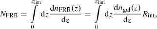
in which zlim is the survey-limiting redshift, dnFRB(z)/dz the rate of observable FRBs with their hosts per square degree per year per redshift interval dz, and dngal(z)/dz is the number density of observable FRB-emitting galaxies per square degree per redshift interval dz. Estimates for the latter have been simulated by Wilman et al. (2008). Their simulation takes into account the observed large-scale clustering effects of galaxies. It uses Poisson sampling of sources from luminosity functions that are based on observed luminosities, which are extrapolated over the redshift range considered in the simulation. The database of all results is publicly available2 and contains about 320 million simulated radio sources of five different types in a 20 × 20 deg2 area from redshift 0 to 20. It is designed to match the technical specifications envisioned for SKA phase 1 and 2 because the 20 × 20 deg2 sky coverage is approximately the largest, it has an instantaneous field of view, and the lower flux density limit of 10 nJy at 1.4 GHz is on the order of the expected detection limit for a 100 h observation with the nominal SKA sensitivity.
We extract all star-forming galaxies within the central square degree of the simulation with z ∈ [0,6] and total fluxes above 10 μJy at 1.4 GHz to ensure that most parts of the host galaxies can be resolved above the detection limit. Figure 1 (left) shows the distribution of potential FRB host galaxies per redshift, dngal(z)/dz, binned in redshift bins of 0.1 width. Figure 1 (right) shows the rate of observable FRBs according to Eq. (2). For this plot, we assume Rint = 10−4 per galaxy per day, which lies between the two values used in Fialkov & Loeb (2017). The resulting 21 FRBs per square degree per year amount to approximately 2300 FRBs per sky per day, which is on the order of the estimates of Fialkov & Loeb (2017). Hence, if Keane & Petroff (2015) and the more recent estimates by Law et al. (2017; and references therein) of approximately 2000 FRBs per sky per day above 1 Jy ms are the total amount of FRBs to be observable, SKA phase 2 is likely to detect the vast majority of them.
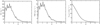 |
Fig. 1. Left panel: distribution of observable FRB host galaxies with total flux above 10 μJy at 1.4 GHz per square degree per redshift, dngal(z)/dz, binned in redshift bins of 0.1 width taken from the SKA Simulated Skies. Middle panel: distribution of potentially observable FRBs from these host galaxies per square degree per year, assuming an internal emission rate of Rint = 10−4 per galaxy per day. Right panel: integrated number of observable FRBs per square degree per year from z to zlim = 6. |
2.2. Probability of a multiply imaged FRB
According to Schneider et al. (1992), the probability of a source at redshift zs being lensed by foreground masses is given by
in which Ds and Dl are the angular diameter distances from the observer to the source at redshift zs and a lens at redshift zl, respectively. σ(M, zl, zs) is the cross section of the lens depending on its mass M and redshift, and n(M, zl)dM is the number density of lenses in the mass range M and M + δM at redshift zl.
To obtain an analytic estimate of the lensing cross section σ(M, zl, zs), we approximate the mass profile of the galaxy clusters as an axisymmetric one with the Einstein radius rE(M, zl, zs) that depends on the mass of the lens, its redshift, and the redshift of the source. The mass inside a tangential critical curve of an axisymmetric lens with an Einstein radius of rE can be approximated by
with Σcr = c2/(4πG)Ds/(DlDls), as derived in Hoekstra et al. (2013).
The cross section is given by the back-projection of the area enclosed by a disk of radius DlrE(M, zl, zs) to the source plane3:
We determine the Einstein radius for a given mass, assuming a Navarro-Frenk-White profile (NFW; Navarro et al. 1996) for the galaxy-cluster scale lenses. This profile generates three multiple images of a source inside the caustic: a maximum close to the lens centre at radius r1, a saddle point on the same side of the lens centre as the maximum at radius r2, and a minimum on the opposite side of the lens centre at radius r3, that is, r1 < r2 < r3. The maximum and the saddle point image straddle the radial critical curve, while the minimum lies outside the tangential critical curve.
The profiles we consider should generate multiple-image configurations with at least 10 arcseconds distance between the minimum and the saddle point image, so that a continuum sky survey of SKA phase 2 can resolve both images. Due to the time delays between the images, the minimum will arrive first, followed by the saddle point image, so that the detection of these two images leaves enough time (on the order of several weeks to months, as estimated in Sect. 2.3) to observe the region of interest at subarcsecond resolution to locate the maximum.
We approximate the angular distance between the minimum and the saddle point by the diameter of the Einstein ring when we determine the lensing probability in Eq. (3). In galaxy clusters, the separations of multiple images that lie on opposite sides of the lens centre usually range from several arcseconds to more than ten arcseconds, giving an estimate for rE. For instance, in CL0024, image separations as large as 30 arcseconds were measured (Broadhurst et al. 2000).
For galaxy-scale lenses of masses less than 1013 M⊙, a singular isothermal sphere (SIS) is usually employed as lens model. The combination of the SIS for the galaxies and the NFW profiles for masses of more than 1013 M⊙ has been shown to match observations well (Li & Ostriker 2002).
To determine the number density of lenses n(M, zl) in a mass interval dM, various analytical and numerical approaches have been established (Jenkins et al. 2001; Linke et al. 2017; Press & Schechter 1974; Sheth et al. 2001; Tinker et al. 2008). Although the halo mass function by Press & Schechter (1974) is often employed, it is known to overestimate the number density of galaxy-size halos and underestimate the number density of galaxy-cluster-scale halos. A comparison of the most common approaches can be found in Linke et al. (2017). They develop an analytical approach to obtain the number density of galaxy clusters taking into account correlated, non-linear structure growth and show that the standard halo-mass functions based on numerical simulations come close to their results. Therefore, we resort to the halo-mass function of Sheth et al. (2001) which is a commonly used standard halo-mass function. Figure 2 (left) shows the halo-mass function for z = 0 (solid line) and z = 1 (dashed line), as obtained by the software described in Murray et al. (2013).
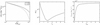 |
Fig. 2. Left panel: halo-mass function according to Sheth et al. (2001) for z = 0 (solid line) and z = 1 (dashed line). Middle panel: lensing probability according to Eq. (3) for zs from 0.1 to 6.0 and NFW halos with a minimum Einstein radius of 5 arcseconds. Right panel: integrated number of observable multiply imaged FRBs per square degree per year from z = 0 out to zlim from 0.1 to 6.0 according to Eq. (6). |
We restrict our calculations to the dark matter halos and neglect the luminous part of the galaxy clusters. In this way, we obtain a lower bound on the probability of multiply imaged FRBs because Hilbert et al. (2008) showed that the probability of lensing is only increased when luminous matter is taken into account.
Combining Eqs. (2) and (3), the overall expected number of multiply imaged FRBs per square degree per year is
The lensing probabilities for sources at zs from 0.1 to 6.0 by NFW profiles with an Einstein radius of at least 5 arcseconds are shown in Fig. 2 (centre). The estimated detection rate of multiply imaged FRBs out to zlim from 0.1 to 6.0 based on the FRB model as outlined in Sect. 2.1 is shown in Fig. 2 (right).
As a rough estimate for the number of repeating FRBs, we could assume that at least 1/60 of all FRBs are repeating, given that FRB121102 is the only repeating FRB out of a sample of 60 detected so far. Consequently, the rate of multiply imaged repeating FRBs could be estimated to be at least 1/60 NmFRB because some of the remaining 59 FRBs could turn into repeating FRBs.
2.3. Estimated time delays and image separations
For cluster-scale lenses, we determine estimates for the expected time delays from an NFW-profile, assuming that the background source is located close to the caustic curve, meaning that we observe the maximum and the saddle point images close to the radial critical curve. Subsequently, as derived in detail in Appendix A, we can approximate the expected time delay between these two images close to the radial critical curve
![$$ \begin{aligned} \tau _\mathrm{f} =&\dfrac{r_\mathrm{s} ^2 D_\mathrm{s} }{c D_\mathrm{l} D_\mathrm{ls} } \left(1+z_\mathrm{l} \right) \left[ \left(r_1 - r_2\right)\left(r_\mathrm{r} + y_\mathrm{r} \right) + \psi (r_2) - \psi (r_1) \right] \nonumber \\ =&1.19 \times 10^9~\text{ d} \dfrac{D_\mathrm{s} (1+z_\mathrm{l} )}{D_\mathrm{ls} } \left[ \dfrac{\pi ^2}{4.20 \times 10^{11}} \left( \dfrac{\theta _1 - \theta _2}{1^{\prime \prime }}\right)\left( \dfrac{\theta _\mathrm{r} + \beta _\mathrm{r} }{1^{\prime \prime }}\right)\right. \nonumber \\&\left. + \dfrac{r_\mathrm{s} }{D_\mathrm{l} } \left( \psi \left( \theta _2\dfrac{D_\mathrm{l} }{r_\mathrm{s} }\right) - \psi \left( \theta _1\dfrac{D_\mathrm{l} }{r_\mathrm{s} } \right) \right) \right], \end{aligned} $$](/articles/aa/full_html/2019/01/aa33530-18/aa33530-18-eq10.gif)
in which the deflection potential ψ(r) is given by
![$$ \begin{aligned} \psi (r) = 4 \kappa _\mathrm{s} \left[ \dfrac{1}{2} \ln ^2 \left( \dfrac{r}{2} \right) + 2 \, \text{ atanh}^2 \sqrt{\dfrac{1-r}{1+r}}\right], \end{aligned} $$](/articles/aa/full_html/2019/01/aa33530-18/aa33530-18-eq11.gif)
and the parameters of the NFW-profile are the scaling convergence κs and the scale radius rs. The radial distance ri = θiDl/rs is the observed angular distance θi from the lens centre to the position of the image i multiplied by the ratio between the angular diameter distance from the observer to the lens plane and the scale radius. The radius of the radial critical curve is denoted by rr and yr = βrDl/rs is its back-projection into the source plane. Expected time delays are thus on the order of 100 days with image separations of a few arcseconds for typical values of κs = 0.2 and rs = 500 kpc, zl = 0.5, and zs = 1.5 (see e.g. Merten et al. 2015 for typical values of κs, rs, zl, and zs).
Analogously, we derive an estimate for the time delay between the saddle point image and the minimum image, which is located close to the tangential critical curve with radius rt
![$$ \begin{aligned} \tau _\mathrm{o}&= \dfrac{r_\mathrm{s} ^2 D_\mathrm{s} }{c D_\mathrm{l} D_\mathrm{ls} } \left(1+z_\mathrm{l} \right) \left[ \dfrac{\left(r_2 - r_3\right)\left(r_\mathrm{t} + r_\mathrm{r} \right)}{2} + \psi (r_3) - \psi (r_2) \right]. \end{aligned} $$](/articles/aa/full_html/2019/01/aa33530-18/aa33530-18-eq12.gif)
The transformation from r to observable angular distances θ is the same as for Eq. (7) and the detailed calculation can also be found in Appendix A. Hence, typical time delays τo are on the order of years for image separations in the range of 10 arcseconds for the same values of κs and rs as used to estimate τf. Measured values for QSOs, as shown in Sect. 4.1, are in agreement with estimates for τf and τo.
2.4. Lensing effects due to smaller-scale structures
For galaxy-scale lenses, we can approximate the lensing mass profile by a SIS and estimate the time delay τ between the two images to be
in which σv is the velocity dispersion along the line of sight, r1 is the observed angular distance from the centre of the lens to the minimum image located outside of the critical curve, and r2 is the observed angular distance from the centre to the saddle-point image inside the critical curve. Measured time delays for QSOs, as listed for instance in Oguri (2007), are usually in the range of days to weeks with image separations on the order of an arcsecond.
As discussed in detail in Zheng et al. (2014), the lensing effects due to intervening massive compact halo objects (MACHOs) will not lead to observable separations between the two images and lead to time delays on the order of 0.1 ms for impact parameters that are approximately equal to the Einstein radius of the MACHO.
Hence, image separations and typical time delays for the different scales of lensing can be distinguished from each other. This is corroborated by observations from quasar lensing. For instance, Oguri (2007) compares observed time delays due to galaxy-scale lenses that are isolated in the field and due to those that are embedded in a cluster environment.
2.5. Discrimination from repeating and independent fast radio bursts
If the luminosity function of the FRBs has a steep slope at the faint end, the main contribution of observed FRBs could come from member galaxies of clusters, as investigated in Fialkov et al. (2018). Hence, precise redshift measurements for the FRBs are necessary in order to distinguish the multiply imaged FRBs originating in background host galaxies from the FRBs of cluster member galaxies.
If the spatial resolution of the telescope is not sufficient to resolve the angular positions of two or three adjacent multiple images in a fold or cusp configuration4, a repeating, temporally resolved signal will be observed, twice for a fold, three times for a cusp.
Repeatedly detected FRBs due to spatially unresolved multiple images have to be distinguished from repeating signals coming from the same source that is not multiply imaged, such as for instance the repeating FRB121102. These two cases can be distinguished by observing the signal from the multiple image on the opposite side of the lens centre after time delays on the order of days to weeks for galaxy-scale lenses and on the order of months to years for cluster-scale lenses.
As FRBs are events of very short duration, resolving the host galaxy before or after the occurrence of an FRB is easier than in the presence of a bright QSO. Thus, a spectroscopic follow-up analysis of the multiply imaged host galaxy at an increased resolution (also in different bands) corroborates the lensing hypothesis for the observed repeating FRB signal. The same spectroscopic test of the host distinguishes multiple images of an FRB from a single source from several FRBs from different hosts.
3. Usage of multiply imaged fast radio bursts
In Sect. 3.1, we discuss the information offered by multiply imaged FRBs on the galaxy cluster at the positions of the multiple images without assuming a specific lens model. Subsequently, in Sect. 3.2, we show benefits of multiply imaged FRBs for global reconstructions of the cluster mass or potential. While the main focus lies on the galaxy-cluster scale lenses, where possible we also comment on the applicability to galaxy-scale lenses. While Sect. 2 was concerned with the detection rates of multiply imaged FRBs and therefore strongly relied on our choice of the underlying FRB model, the findings of Sect. 3 are based on general principles of the gravitational lensing formalism and can be applied to any transient multiply imaged source.
3.1. Model-independent, local information gain
The time delay τij between two multiple images i and j of an FRB located at angular position y in the source plane is given by
with measured angular positions xi of the two images in the lens plane and the lensing potential ϕ(y, x), as defined in Appendix A. Using Eq. (11), we can infer the difference in lensing potentials between the two positions, Δϕ(y,xi,xj), without inserting a specific lens model, for a fixed cosmological model that determines the distances Dl, Ds, Dls along the line of sight. Vice versa, if Δϕ and its dependence on the cosmological model is known, we can determine properties of this cosmological model, for example the Hubble constant H0 or the matter density parameter Ωm0 in a Friedmann model, as detailed in Grillo et al. (2018) for example.
Knowing neither the underlying cosmology nor Δϕ, Eq. (11) is subject to a degeneracy: we can scale D by an arbitrary factor λ ∈ ℝ. At the same time, Δϕ is subject to the mass sheet degeneracy (see Liesenborgs & De Rijcke 2012; Schneider & Sluse 2014 and references therein) stating that Δϕ can also be scaled by an arbitrary factor  , while leaving the observables invariant. For
  , the measured time delay remains invariant.
This degeneracy is broken, if the distances Dl and Ds can be measured. Subsequently, Δϕ can be determined from Eq. (11), which becomes feasible if FRBs turn out to be standardisable candles. Observing a multiply imaged FRB and an FRB from a cluster member galaxy, the positions of the lens and the source along the line of sight with respect to the observer can be fixed. This is true for any combination of observed standardisable candles, for instance for a multiply imaged SN coinciding with an FRB from the image plane. However, the latter case seems less frequent (see Sect. 4.2) and it remains to be shown that FRBs can be standardised.
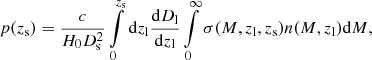
As shown in Wagner (2017), we can approximate Eq. (11) for two images that straddle a critical curve by
with δx = δθDl/rs being the rescaled measured angular separation between the two images. The third-order derivative in x2-direction  is determined at the position x0 = 1/2(xi + xj) in the coordinate system in which the multiple images are stretched along the x2-direction. Figure 3 shows the ratio of τ≈ to τ for the two multiple images at the radial critical curve of an NFW profile, that is, δx = r1 − r2, with typical values of κs for rs = 0.5 Mpc.
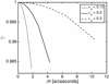 |
Fig. 3. Accuracy of the approximation of the time delay: ratio between τ≈, Eq. (12), and τ, Eq. (11), for the two images straddling the radial critical curve in NFW profiles with rs = 0.5 Mpc for κs = 0.15 (dotted curve), κs = 0.2 (solid curve), and κs = 0.3 (dashed curve) vs. the observed angular separation of the two images δθ = (r1 − r2)rs/Dl. |
Instead of Δϕ, that is, the potential difference between two points in the image plane, we can determine  at a single point from the measured time delays and image separation by Eq. (12). This may be more convenient for some global lens reconstruction algorithms, as discussed in Sect. 3.2.
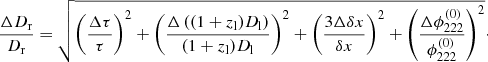
All results obtained in this section can be applied to multiple images of any time-varying source and generated by galaxy-scale or cluster-scale lenses. For both scales, the precision with which Δϕ or  can be determined by Eqs. (11) and (12) is dominated by the uncertainties in the distances D, and for Eq. (12) also by the angular separation δx. Assuming an FRB as the source with uncertainties of 1 ms for time delays of 100 days, the relative uncertainty is on the order of 10−10. Assuming typical lens and source redshifts of zl = 0.5 ± 0.01 and zs = 1.5 ± 0.01, the relative uncertainty of D – only considering the imprecision on z and neglecting the uncertainties in the cosmological parameters – is of the order of 2–3% and the relative uncertainty of δx is usually just below 1%, meaning that the time delay is the most precise quantity, which is not the case for the other time-varying sources (see Table 4 for a comparison).
For repeating bursts from the same source, we can measure the time delays between the multiple images several times. Significant deviations between the results indicate a change in the potential difference, δ(Δϕ). Given that the absorption properties of the intracluster gas and other extinction effects do not change and the emission properties of the source remain the same, this difference could be attributed to small-scale structure, as detailed in Sect. 2.4, that enters and leaves the light paths of the multiple images between the repetitions.
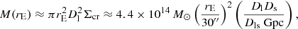
To study the change in time delays caused by small-scale structure moving in and out of the galaxy cluster potential, ϕ, we consider a change in the virial mass ΔMvir of the NFW profile of Sect. 2.3 from 105 to 1012 solar masses. Figure 4 shows the change in the time delay, Δτ, between the repeating multiply imaged FRBs close to the radial critical curve for different angular distances between the multiple images. The figure shows that depending on the distance between the images, a change in the virial mass of 105 M⊙ between the repetitions of the FRBs can be detected. Determining the change in the angular distances for increasing changes in mass, we find them to be on the order of 10−9, 10−8, and 10−3 arcseconds, too small to be observed. Altogether, we find that changes in the time delay due to a change in the cluster mass between FRB repetitions cannot be used to detect MACHOs of a few solar masses and repetition and observation times are much too short to track the motion of larger objects such as galaxies.
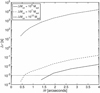 |
Fig. 4. Difference between time delays of repeating multiply imaged FRBs for increasing angular distances at the radial critical curve of the NFW profile of Sect. 2.3 when the virial mass of the NFW profile is increased by 105 solar masses (solid line), by 107 solar masses (dashed line), and by 1012 solar masses (dash-dotted line). The measurement precision of τij for one measurement, approximately 1 ms, is shown as a dotted line. |
3.2. Information gain in global lens reconstructions
3.2.1. Time-delay constraints in different lens reconstruction algorithms
Reconstructions of the lensing mass distribution from several sets of multiple images in a galaxy cluster are obtained by parametric methods such as Lenstool (Kneib et al. 1996; Jullo et al. 2007), the approach by Grillo et al. (2015), non-parametric approaches on a grid, such as Grale (Liesenborgs et al. 2010), or model-free and mesh-free approaches such as SaWLens (Merten 2016). As time delays in galaxy clusters are rarely available, Lenstool does not provide the ability to use time delays as constraints for the reconstructions of the lens.
In SaWLens, constraints from time delays are also not implemented yet. This mesh-free algorithm sets constraints to the lensing potential and its derivatives in the form of a χ2-minimisation term at positions where observables are available. As Eq. (11) cannot be assigned to a single point, it will require some extension of the algorithm to include this constraint. But it is easy to use Eq. (12) for all time delays of multiple images i, j that straddle a critical curve by adding
to the already existing χ2 terms.
Grillo et al. (2018) includes time delays in the approach of Grillo et al. (2015) to determine the posterior probability density function of cosmological parameters. The Bayesian parameter estimation employs a Gaussian likelihood for a given 
in which the sum is taken over all image pairs (i, j) with measured time delays τij. The measurement uncertainty for each τij is denoted by στij and  is the model-predicted time delay between the images. The latter is determined by Eq. (11) after inserting a cosmological model to determine D and a lens model to determine Δϕ. A joint reconstruction from all multiple images of the source, as detailed in Suyu et al. (2006), is employed to determine the source position that is inserted into Δϕ. Instead of constraining cosmological parameters with this approach, the time delays could be used to improve the reconstruction of the lensing potential as described in Sect. 3.1.
Liesenborgs et al. (2009) and Liesenborgs & De Rijcke (2012) investigated how time delays improve the reconstruction of the lensing mass distribution. They implemented a term in the optimisation routine of Grale that minimises the difference between the time delay predicted by the lens model and the observed one as follows:
in which the first and second sum are taken over all pairs of images (i, j) of a source for which a time-delay measurement, τij, is available. The last two sums are taken over all N multiple images. As the source position is unknown, the back-projected image positions, yk and yh, are employed. Subsequently,  searches for the minimum difference between the arrival times t for all image pairs (i, j) and the observed time delay τij. Due to the weighting of all time delays by the duration of the measured time delay, time delays of all lengths are treated equally. As yk and yh are not necessarily equal, a bias is introduced that may affect the reconstructed time delay. This will be the subject of a more detailed, future investigation of the general form of
  and a comparison to the other approaches.
3.2.2. Reconstructing a simulated cluster-scale lens with Grale including time delays
For a simulated example of a generalised NFW profile, Liesenborgs & De Rijcke (2012) used time delays of one set of three multiple images to demonstrate that time delay information greatly alleviates the mass sheet degeneracy in their lens reconstruction. They compared lens models based on the constraints of positions of 26 multiple images from eight sources with zs ∈ [2.7, 3.4] with and without an additional mass-sheet basis function, with and without the three time-delay constraints between the three multiple images. We extend their analysis and investigate the reconstruction accuracy for the mass density distribution when only one time-delay constraint is available, with and without adding an additional mass sheet. Instead of 20 models, we average over 30 individual reconstructions from the genetic algorithm. However, a systematic investigation performed in Wagner et al. (2018) shows that the effect on the standard deviations is negligible, which can be corroborated comparing the plots in the top row of Fig. 6 with corresponding ones in Liesenborgs & De Rijcke (2012).
We summarise all Grale models with the different constraints in Table 1. Figures 5, 6, and 7 show the reconstruction results of these models starting with model 1 from top left and ending with model 8 at the bottom right.
 |
Fig. 5. Comparison between Grale lens models for the simulated, generalised NFW profile that is detailed in Liesenborgs & De Rijcke (2012). Each map shows the reconstructed critical curves (red, solid lines) and the reconstructed caustics (blue, solid lines) together with the true critical curves (black, dashed lines) for the Grale models with the same constraints detailed in Table 1 and Fig. 7 (i.e. the left and right columns show models without and including an additional mass-sheet basis function, respectively). Top left panel: model includes no additional mass sheet and no timedelay constraints. Top right panel: using an additional mass sheet. Second row, left: including time-delay constraints between the three multiple images marked by the black dots. Second row, right: as in the left-hand side but using an additional mass sheet. Third row, left: including one time-delay constraint between the multiple images marked by the black dots. Third row, right: as in the left-hand side but with an additional mass sheet. Fourth row, left: same as above but for a different pair of multiple images. Fourth row, right: as for the left-hand side but with an additional mass sheet. |
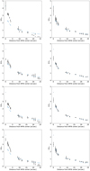 |
Fig. 6. Comparison between Grale lens models for the simulated, generalised NFW profile that is detailed in Liesenborgs & De Rijcke (2012). Each plot shows the reconstructed convergence values and their uncertainties (black points with error bars) and the true convergence values (blue points) at the positions of the multiple images measured as radial distance from the centre of the NFW profile for the Grale models with the same constraints as detailed in Table 1 and Fig. 5. |
 |
Fig. 7. Comparison between Grale lens models for the simulated, generalised NFW profile that is detailed in Liesenborgs & De Rijcke (2012). Each map shows the difference between the reconstructed convergence map and the simulation result for the models with the same constraints as detailed in Table 1 and Fig. 5. The circles mark the positions of the multiple images and their size is proportional to the difference between the reconstructed and real convergence at these positions. The white circles indicate the multiple images with the time-delay constraints. For the multiple images marked by red circles, no time-delay constraint is given. |
Comparing the results for the reconstructed critical curves between the different models, Fig. 5 shows that the inclusion of an additional mass sheet improves the reconstruction accuracy, has a smoothing effect on the critical curves, and leads to less complex and more accurate caustics. These results are in agreement with the findings of Liesenborgs & De Rijcke (2012) and occur because the Plummer basis functions alone can hardly account for an overall offset in the mass density distribution, a mass-sheet basis function alleviates this. Comparing the reconstructed critical curves for models 4 and 6, Fig. 5 shows that both are of comparable quality, while the reconstructed critical curves for model 8 are of minor quality with additional critical curves in the central part and larger deviations between the true and the reconstructed inner critical curve. These results can be explained by the fact that the multiple images with the time-delay constraint in model 8 lie very closely together and yield a more local constraint than the time-delay constraints in models 6 or 4. For the same reason, the reconstruction of the inner critical curve in model 8 is accurate only in the vicinity of the two multiple images with the time-delay constraint.
Consistent results for the reconstruction of the convergence are found in Fig. 6. The plots show the true and the reconstructed convergences at the radial distances of the multiple images from the centre of the NFW profile for all models. Adding a mass sheet to the Plummer basis increases the reconstruction accuracy, as can be observed when comparing models with odd numbers (left-hand side of Fig. 6) and models with even numbers (right-hand side of Fig. 6). Taking into account time-delay constraints without adding a mass sheet increases the overall accuracy but the reconstruction is biased towards a less cuspy profile in the centre. Three time-delay constraints yield the highest accuracy (model 3), followed by the time-delay constraint of the two multiple images with farthest distance (model 5), and then followed by the time-delay constraint of the two multiple images that lie closely together (model 7). Adding a mass sheet the accuracy is further increased, except for model 8, but it does not alleviate the bias. This bias might originate from the sparse density of constraints in favour of a cuspy centre because the distribution of basis functions over the cluster region is similar to that of the first two models, which are able to reconstruct the steep slope in the centre of the cluster.
Comparing the standard deviations between the models, we observe that including the time-delay constraints, and thus reducing the degrees of freedom, reduces the differences between the individual reconstructions obtained from the genetic algorithm. Due to the locality of the time-delay constraint in models 7 and 8, their standard deviations are increased compared to the other models with time-delay constraints. For the latter models, the standard deviations are comparable with each other. Comparing the standard deviation between the reconstructions obtained from the genetic algorithm (i.e. the reconstruction precision) with the differences between the true convergence value and the reconstructed value (i.e. the reconstruction accuracy) in the entire field, we find that both are of the same order of magnitude.
Figure 7 shows the map of differences between the reconstructed convergence values and the true values over the entire region of the simulation. As already observed in Figs. 5 and 6, including time-delay constraints increases the reconstruction accuracy of the lensing mass distribution and adding a mass sheet reduces the deviations further.
To investigate the accuracy to which the time delays between the images are recovered for models 1 to 8, we proceed as follows: for each individual model, the source position is estimated as the average of the back-projected image positions. For this source position, updated image positions are calculated, in order to circumvent the bias that Eq. (15) is subject to. Then, time delays are determined between these image positions. For all 30 time delays per image pair of the individual reconstructions, the average and its standard deviation are calculated as summarised in Table 2 for the three image pairs in all models 1 to 8. Comparing these time delays to our estimates for time delays of NFW profiles in Sect. 2.3, we find that our time delays are shorter because we use parameter values that are comparable to observed ones, while the simulated lens of Liesenborgs & De Rijcke (2012) has a higher concentration parameter. The scale radius is of comparable size.
Comparing the reconstructed time delays for the different models listed in Table 2, we conclude that, as expected, the time delays are retrieved very accurately when using them as constraints. In addition, we find that adding a mass sheet is necessary to reconstruct most of the time delays correctly because time delays break the mass-sheet degeneracy. Only the time delays τ12 and τ13 cannot be correctly reconstructed within the range of their standard deviations in model 8. Leaving these time delays aside, we observe that the standard deviation of the reconstructed time delay due to the variation in the individual reconstructions by the genetic algorithm is reduced by about one order of magnitude when time-delay constraints from the remaining pair of multiple images for that source are included in the lens reconstruction, except for Δτ23 in model 6. For another visualisation, three-dimensional plots of the maps in Fig. 7 are available online5. Equation (15) assumes that measurement uncertainties of the time delays are negligible, meaning that the results shown in Fig. 7 resemble those that are obtainable with FRBs.
On the whole, this example shows that even a single time-delay measurement improves the accuracy of the lens reconstruction. If the pair of images consists of a minimum and a saddle point lying on opposite sides of the lens centre, the reconstruction accuracy for the convergence in the entire region around the galaxy cluster core is of comparable quality as if time-delay constraints between three multiple images had been employed.
3.2.3. Using time delays to determine the Hubble constant
Galaxies can be phenomenologically described by power-law volume mass density profiles, ρ(R)∝R−γ, which is supported by observations of galaxy dynamics, X-ray emissions, and strong lensing measurements. By assuming the power-law profile, the mass sheet degeneracy is broken. This may introduce a bias, for example in the determination of H0 from Eq. (11) (Sonnenfeld 2018; Xu et al. 2016). However, selecting galaxies that have an approximately isothermal density profile (i.e. with a power-law index γ ≈ 2), simulations analysed in Sonnenfeld (2018) and Xu et al. (2016) showed that the bias can be reduced and H0 determined with less than 5% inaccuracy. Hence, assuming a power-law density profile as lens model, time-delay measurements between multiple images caused by a galaxy-scale lens can be used to probe cosmology by means of Eq. (11).
For galaxy clusters, the deflecting mass-density profile is much more complex, meaning that the bias caused by breaking the mass sheet degeneracy with a lens model can be larger than for galaxies (see Meneghetti et al. 2017 for the precision and accuracy of local lens properties obtained by the most common lens reconstruction approaches). In addition, the cosmological model need not enter as a simple scale factor of the lens potential as is the case for some galaxy-scale lens models. Therefore, galaxy clusters seem to be less suitable for determining H0 compared to galaxy-scale lenses. Nevertheless, Vega-Ferrero et al. (2018) and Grillo et al. (2018) determined H0 from the SN Refsdal behind the galaxy cluster MACS1149 with 17% and 6% imprecision, respectively. In the same way, H0 could be determined from multiply imaged FRBs as well.
4. Comparison to other time-varying sources
In this section, we compare the expected abundances of multiply imaged QSOs, SNe, and GRBs behind galaxy clusters under their most favourable observation conditions in different bands. In addition, we compare the precision and accuracy of the time delays obtained for these time-varying sources with the precision and accuracy achievable by FRBs. For these comparisons, we rely on the FRB-model assumptions as stated in Sect. 2.1, meaning that these estimates should be treated with caution given the limited knowledge of the currently available FRB properties. Nevertheless, our estimates are conservative in the sense that we choose an FRB model with low detection rates, requiring SKA phase 2 for the observation.
4.1. Quasars
Estimated abundances of multiply imaged QSOs with image splittings of at least 10 arcseconds are 8 in 8000 deg2 when considering lensing by dark matter only for QSOs up to zs = 5 using the specifications of the SDSS photometric survey (Hennawi et al. 2007). Including the influence of the brightest cluster galaxy, the rate increases to 12 in 8000 deg2. Assuming a data collection time on the order of 10 years, the estimated detection rate is 1.5 × 10⁻⁴ multiply imaged QSOs per square degree per year. This result is of the same order as the 1.3 × 10⁻⁴ multiply imaged FRBs per square degree per year up to zs = 5.
The photometrical variability of QSOs is on the order of a few days (Bonvin et al. 2016). Apart from the time scale of the intrinsic variability, the precision of a time-delay measurement also depends on the cadence of the observations as investigated by Liao et al. (2015) for simulated time delays caused by galaxy-scale lenses. In Liao et al. (2015), cadences on the scale of 3 days are considered, meaning that imprecisions of the time-delay measurements are on the order of 1–2 days at best.
Liao et al. (2015) find that the best algorithms obtain time delays with sub-percent inaccuracy and 3% imprecision, yet the rate of light curves from which time delays could be retrieved was only around 50% of all those simulated. For current observational data, as collected in Oguri (2007), the precision is on the order of 90% for galaxy-scale lenses. Table 3 lists the observed multiply imaged QSOs in galaxy clusters together with the largest image separation and measured time delays. The table shows that there is high variability in measurement uncertainties ranging from sub-percent level to over 10% with absolute uncertainties on the order of the cadence mentioned above.
Synopsis of observed multiply imaged QSOs with their largest image separation δθ and measured time delays τ.
Hence, assuming an uncertainty of 1.5 days for measured time delays of 100 days of QSOs, the relative uncertainty amounts to 0.015, which is several orders of magnitude larger than for FRBs (see Sect. 2.3) and not negligible compared to the uncertainties of the other observables.
4.2. Supernovae
The abundance of multiply imaged SNe observable behind massive galaxy clusters is estimated in Gunnarsson & Goobar (2003). They consider an NFW profile of virial mass 2 × 10¹⁵ M⊙ located at zl = 0.2 and sources in the redshift range zs ∈ [1.5,5]. These configurations cover minimum image splittings in the range of 6–21 arcseconds depending on zs. For observations in the J-band, they expect 7–10 multiply imaged type-Ia SNe per cluster per year and 21–24 multiply imaged type-II SNe per cluster per year. These numbers are rough estimates because, similarly to the FRB rates, the SN rates, especially at high redshifts, are not known (see Sect. 2.1). Improved searching criteria, as discussed in Goldstein & Nugent (2017) may lead to better-constrained abundance estimates in the future.
As further detailed in Appendix B, the total number of about 30 SNe per cluster per year translates to an estimated detection rate of 2.34 × 10⁻⁵ multiply imaged SNe per square degree per year. For comparison, we determine the detection rate of multiply imaged FRBs with source redshifts zs ∈ [1.5,5] that are caused by clusters of 2 × 10¹⁵ M⊙ at lens redshift zd, which amounts to 5.51 × 10⁻⁹ multiply imaged FRBs per square degree per year. Hence, we expect less FRBs than SNe given the limited range of redshifts of Gunnarsson & Goobar (2003).
The distribution of observable FRB-emitting galaxies peaks around z = 1 and decreases quickly for z > 1.5. Therefore, a much more significant comparison would extend the calculations for the SNe to smaller redshifts and a broader range of cluster masses. However, to our knowledge, these calculations are still in preparation for large surveys and are not yet available. Furthermore, the numbers given in Gunnarsson & Goobar (2003) do not take into account that SNe are only visible for about 100 days. From the estimated numbers of SNe and QSOs behind galaxy-scale lenses, as discussed in Oguri & Marshall (2010), we find, for example, that the predicted detection rates of multiply imaged QSOs per year per square degree are more than one order of magnitude higher than those for SNe for the Large Synoptic Survey Telescope (LSST). Extrapolating from these results to the galaxy-cluster lensing regime, we can assume that both rates will be scaled-down by the same lower probability of the sources lying behind a galaxy cluster. Hence, we conclude that the detectable rate of multiply imaged SNe for a broader range of lens redshifts and masses could be lower than the rate of detectable multiply imaged QSOs and FRBs.
The sole, serendipitously found, multiply imaged SN with image splittings of 2 arcseconds and measured time delays (Kelly et al. 2016; Rodney et al. 2016) indicates that uncertainties in time-delay measurements are on the order of days, amounting to more than 28% of the measured time delays6. Among the effects causing this high uncertainty is microlensing, as discussed by Goldstein et al. (2018), which is a disadvantage of using SNe compared to FRBs. We also expect the measurements of time delays between multiple images of a SN to be less precise than those between multiple images of a QSO due to the limited lifetime of SNe.
4.3. Gamma-ray bursts
Gamma-ray bursts are divided into two classes: short-duration GRBs lasting less than 2 s and long-duration GRBs lasting more than 2 s. Only 30% of all GRBs belong to the first group and the observed cases have a mean redshift around z = 0.5, while the mean redshift of all observed long-duration GRBs is around z = 2.0 (Berger 2014). Therefore, we focus on the latter class and, unless stated otherwise, GRB refers to a long-duration GRB.
Chary et al. (2002) find that starburst galaxies are likely to host GRBs. In order to estimate the number of multiply imaged GRBs by galaxy-cluster lenses which also have observable hosts in the radio band, we extract all starburst galaxies from the central square degree simulated in Wilman et al. (2008) with the same specifications as in Sect. 2.1. Their distribution over the redshift range z ∈ [0,6] is shown in Fig. 8 (left). Processing them analogously to the star-forming galaxies (see Sects. 2.1 and 2.2), we obtain the distribution of GRBs (see Eq. (2)) and multiply imaged GRBs (see Eq. (6)), as shown in the central and right-hand panels of Fig. 8, respectively. As internal emission rate, we employ Rint = 10−4 per galaxy per day7 as for the FRBs and Rint = 10−5 per galaxy per year, as is the estimated rate for our Galaxy. A comparison of both values shows that even for an internal emission rate as high as for the FRBs, the number of observable multiply imaged GRBs with their hosts is one order of magnitude smaller than that for FRBs. For the more realistic Rint = 10−5 per galaxy per year, the expected number of multiply imaged GRBs is even five orders of magnitude smaller.
 |
Fig. 8. Left panel: distribution of observable GRB starburst host galaxies with total flux above 10 μJy at 1.4 GHz per square degree, per redshift, dngal(z)/dz, in redshift bins of 0.1 width taken from the SKA Simulated Skies. Middle panel: integrated number of observable GRBs per square degree per year from z to zlim = 6 assuming an internal emission rate of Rint = 10−4 per galaxy per day (solid line) or Rint = 10−5 per galaxy per year (dashed line). Right panel: integrated number of observable multiply imaged GRBs per square degree per year out to zlim from 0.1 to 6.0 according to Eq. (6). |
Therefore, compared to all other time-varying sources, the abundance of multiply imaged GRBs is the smallest, but observing a multiply imaged GRB, the probability that we will also observe a core-collapse SN in its vicinity is increased (Hjorth et al. 2012).
As the spatial resolution of gamma-ray telescopes is limited to approximately 0.1° by their detection mechanism, the localisation precision is too low to identify multiply imaged GRBs as such. Instead, they are detected by light-curve matching as further detailed in Barnacka et al. (2015) and Davidson et al. (2011). Being able to observe an afterglow in X-ray or optical and radio bands, the localisation precision is increased to 10 arcseconds and subarcseconds, respectively (Prochaska et al. 2006). Due to these difficult observation and detection conditions, only two multiply imaged GRBs caused by galaxy-scale lenses have been detected so far (Barnacka et al. 2015, 2016).
Given uncertainties of 0.5 days for these two observed cases, the expected imprecision of time delays in the galaxy cluster regime with time delays on the order of 100 days is 0.5%. Hence, the precision is higher than those of QSOs (see Table 4).
Results of the comparison between different time-varying, multiply imaged sources behind galaxy clusters.
5. Redshifts for FRBs based on gravitational lens models
If the FRB and its host are positioned at such a high redshift that the peak flux of the FRB is close to the sensitivity limit of the detector and the host galaxy is below it, the latter can no longer be observed. Consequently, the redshift of the FRB cannot be determined from the spectrum of the host. For this case, a gravitational lens model can be employed to determine the (comoving) cosmic distance to the FRB or its redshift:
Assuming the time delay between two adjacent multiple images in a fold configuration, τ, the distance between these two images δx, and the redshift of the lens were measured, we rewrite Eq. (12)
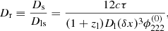
in order to estimate the uncertainty up to which we can determine the distance to the emitted FRB. The value of  is obtained from a global, model-based reconstruction of the gravitational lensing potential or its second-order derivatives (see e.g. Grillo et al. 2015; Jullo et al. 2007; Liesenborgs et al. 2010; Merten 2016). A Gaussian propagation of the uncertainties of the observables in Eq. (16) leads to a relative uncertainty of Dr given by
In addition, the derivation of Eq. (2) of Wagner (2017) involves a Taylor expansion around x0 which adds a systematic bias of less than 2% to the measurement uncertainty (see Fig. 3).
Typical values for the observables of two images of an FRB in a galaxy cluster are τ = 100 d, δx = 5″, and zl = 0.5 with uncertainties Δτ = 1 ms, Δδx = 0.01″, and Δzl = 0.01, which yield
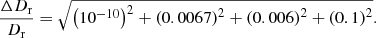
The dominant source of uncertainty is therefore the lens model, if the uncertainty in  is on the order of 10%. We can neglect the uncertainty in τ, zl, and Dl and solve Dr for the comoving distance to the FRB
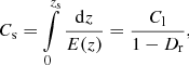
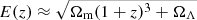
in which E(z) is the expansion function of the universe8, Cl the comoving distance to the lens, and Dr is given by the expression on the right-hand side of Eq. (16). Thus, ΔCs/Cs = ΔDr/(1 − Dr), so that the uncertainty in Cs is approximately 10%, mainly caused by the uncertainty of the lens model for typical redshifts of sources and lenses.
Alternatively, the approach developed in Kneib et al. (1996) and Jullo et al. (2007) determines the most probable parametric lens model in a Markov-Chain-Monte-Carlo optimisation and simultaneously constrains unknown redshifts of multiple images. The user can set a uniform or a Gaussian prior on the redshift and set boundary values or a mean and a standard deviation, respectively. In this way, the redshift of the FRB can be determined to a predefined precision.
6. Conclusion
Using the spectral properties of the repeating FRB121102 as a model, we estimated the rate of multiply imaged FRBs behind galaxy-cluster-scale gravitational lenses detectable by a SKA-phase-2-like telescope. We found the detection rate to be on the order of 10−4 per square degree per year. Comparing this rate with the observation rates of other multiply imaged time-varying sources, as summarised in Table 4, we find that FRBs could be as frequent as multiply imaged QSOs and more frequent than multiply imaged SNe. The least likely time-varying source that will be found behind cluster-scale lenses are GRBs. Table 4 also lists the number of already observed multiple images, the (estimated) uncertainty of the time-delay measurement, the time scale of their duration and whether they may even repeat and be subject to microlensing. The underlying assumptions to obtain these estimates are detailed in Sects. 2.1 and 4. From these findings, we conclude that FRBs could confer many advantages compared to the other time-varying sources because (1) they could be as frequent as QSOs but are not subject to microlensing due to their short duration time and they do not outshine the host galaxy for more than milliseconds, meaning that the host can be resolved more easily, (2) they might also be calibrated to be standard candles but with a higher detection rate than SNe and with a higher precision in the time-delay measurement, and (3) the time delay could be measured several times for repeating FRBs. These advantages are based on the assumptions stated in Sect. 2.1, which, due to the limited amount of observations, may not hold. Nevertheless, the main advantage that they are transients of short duration and subsequently allow us to observe the properties of their hosts remains true and makes them very valuable probes of the mass distribution in a gravitational lens.
Fast radio bursts also carry disadvantages however, due to their short duration time, they require a different detection technique. In a recent wide-field observation, the Australian Square Kilometre Array Pathfinder detected 19, most probably non-repeating FRBs (Shannon et al. 2018). Almost doubling the amount of known FRBs so far, this survey demonstrated that the usage of a fly’s-eye configuration of 5–12 antennas pointing in different directions is very efficient to locate FRBs. In this configuration, the location precision is 10 arcminutes times 10 arcminutes. An ideal configuration to detect multiply imaged FRBs is a continuum all-sky SKA-phase-2-like survey with angular resolution of about 10 arcseconds, which detects the first two multiple images. Subsequently, a high-resolution follow-up observation is necessary to detect and locate further image(s). Additional optical and infrared observations may also be of use to investigate the host galaxy in further detail. To match these requirements, galaxy-cluster-scale gravitational lenses are more suitable than galaxy-scale lenses because cluster lenses cause angular separations between multiple images on the order of 10 arcseconds and time delays on the order of 100 days, which leaves enough time to prepare the high-resolution follow-up observation.
Given that the observational requirements could be fulfilled in the future, multiply imaged FRBs could be used to increase our knowledge of the local and global properties of galaxy clusters and increase the precision of the results by orders of magnitude. In particular, we showed that it is possible to (1) determine differences in the gravitational lensing potential between all positions of multiple images to a greater precision than currently possible; (2) globally alleviate the mass sheet degeneracy in the reconstructions of the mass density profiles based on lens models; (3) determine cosmological parameters to a higher precision than currently possible; (4) determine the redshift or the distance of a very faint, FRB-emitting host galaxy and (5) determine changes in the cluster mass of more than 105 M⊙ from repeating FRBs.
As found for the simulated galaxy-cluster scale lens in Sect. 3.2, the overall reconstruction accuracy for the surface mass density distribution is increased when taking time-delay constraints into account, but this may come at the cost of introducing a bias towards shallower slopes in the cluster core (see Fig. 6). With one time-delay constraint coming from a pair of multiple images from opposite sides of the lens centre, approximately the same reconstruction accuracy in the surface mass density distribution map can be achieved as for the three time-delay constraints from three multiple images.
Although the determination of H0 from SN Refsdal (Vega-Ferrero et al. 2018; Grillo et al. 2018) is an important achievement, we are in favour of putting more emphasis on the analysis of the cluster lensing potential by means of the high-precision time delays. Understanding the degeneracies of the lensing formalism and the lens models, as pointed out by Schneider & Sluse (2014), Liesenborgs & De Rijcke (2012), Unruh et al. (2017), Wertz et al. (2017), and Wagner (2018), for example, may also contribute to resolving the 3-σ tension in the determination of H0 as found by Planck Collaboration XIII (2016), Riess et al. (2016, 2018).
See Schneider et al. (1992), Wagner (2017) for a detailed characterisation of both configurations.
The time delay between the multiple images of the SN on galaxy-cluster scale is not yet measured but only estimated to 345 days in Grillo et al. (2018).
Acknowledgments
We would like to thank Claudio Grillo, Eric Jullo, Julian Merten, Adi Zitrin, and the Galaxy Cluster Group at the Institute for Theoretical Astrophysics for helpful discussions and comments. JW gratefully acknowledges the support by the Deutsche Forschungsgemeinschaft (DFG) WA3547/1-1 and WA3547/1-3. JL acknowledges the use of the computational resources and services provided by the VSC (Flemish Supercomputer Center), funded by the Research Foundation - Flanders (FWO) and the Flemish Government – department EWI. DE acknowledges support from the Israel – U.S. Binational Science Foundation, the Israel Science Foundation including an ISF-UGC grant, and the Joan and Robert Arnow Chair of Theoretical Astrophysics.
References
- Bannister, K. W., Shannon, R. M., Macquart, J.-P., et al. 2017, ApJ, 841, L12 [NASA ADS] [CrossRef] [Google Scholar]
- Barnacka, A., Geller, M. J., Dell’Antonio, I. P., & Benbow, W. 2015, ApJ, 809, 100 [NASA ADS] [CrossRef] [Google Scholar]
- Barnacka, A., Geller, M. J., Dell’Antonio, I. P., & Zitrin, A. 2016, ApJ, 821, 58 [NASA ADS] [CrossRef] [Google Scholar]
- Bassa, C. G., Tendulkar, S. P., Adams, E. A. K., et al. 2017, ApJ, 843, L8 [NASA ADS] [CrossRef] [Google Scholar]
- Behroozi, P. S., Wechsler, R. H., Wu, H.-Y., et al. 2013, ApJ, 763, 18 [NASA ADS] [CrossRef] [Google Scholar]
- Berger, E. 2014, ARA&A, 52, 43 [NASA ADS] [CrossRef] [Google Scholar]
- Bonvin, V., Tewes, M., Courbin, F., et al. 2016, A&A, 585, A88 [NASA ADS] [CrossRef] [EDP Sciences] [Google Scholar]
- Broadhurst, T., Huang, X., Frye, B., & Ellis, R. 2000, ApJ, 534, L15 [NASA ADS] [CrossRef] [Google Scholar]
- Chary, R., Becklin, E. E., & Armus, L. 2002, ApJ, 566, 229 [NASA ADS] [CrossRef] [Google Scholar]
- Chatterjee, S., Law, C. J., Wharton, R. S., et al. 2017, Nature, 541, 58 [NASA ADS] [CrossRef] [Google Scholar]
- Cordes, J. M., Wasserman, I., Hessels, J. W. T., et al. 2017, ApJ, 842, 35 [NASA ADS] [CrossRef] [Google Scholar]
- Dahle, H., Gladders, M. D., Sharon, K., et al. 2013, ApJ, 773, 146 [NASA ADS] [CrossRef] [Google Scholar]
- Dahle, H., Gladders, M. D., Sharon, K., Bayliss, M. B., & Rigby, J. R. 2015, ApJ, 813, 67 [NASA ADS] [CrossRef] [Google Scholar]
- Dai, L., & Lu, W. 2017, ApJ, 847, 19 [NASA ADS] [CrossRef] [Google Scholar]
- Davidson, R., Bhat, P. N., & Li, G. 2011, in AIP Conf. Ser., eds. J. E. McEnery, J. L. Racusin, & N. Gehrels, 1358, 17 [NASA ADS] [Google Scholar]
- Eichler, D. 2017, ApJ, 850, 159 [NASA ADS] [CrossRef] [Google Scholar]
- Fialkov, A., & Loeb, A. 2017, ApJ, 846, L27 [NASA ADS] [CrossRef] [Google Scholar]
- Fialkov, A., Loeb, A., & Lorimer, D. R. 2018, ApJ, 863, 132 [NASA ADS] [CrossRef] [Google Scholar]
- Fohlmeister, J., Kochanek, C. S., Falco, E. E., Morgan, C. W., & Wambsganss, J. 2008, ApJ, 676, 761 [NASA ADS] [CrossRef] [Google Scholar]
- Fohlmeister, J., Kochanek, C. S., Falco, E. E., et al. 2013, ApJ, 764, 186 [NASA ADS] [CrossRef] [Google Scholar]
- Goldstein, D. A., & Nugent, P. E. 2017, ApJ, 834, L5 [Google Scholar]
- Goldstein, D. A., Nugent, P. E., Kasen, D. N., & Collett, T. E. 2018, ApJ, 855, 22 [NASA ADS] [CrossRef] [Google Scholar]
- Goobar, A., Amanullah, R., Kulkarni, S. R., et al. 2017, Science, 356, 291 [Google Scholar]
- Grillo, C., Suyu, S. H., Rosati, P., et al. 2015, ApJ, 800, 38 [NASA ADS] [CrossRef] [Google Scholar]
- Grillo, C., Rosati, P., Suyu, S. H., et al. 2018, ApJ, 860, 94 [NASA ADS] [CrossRef] [Google Scholar]
- Gunnarsson, C., & Goobar, A. 2003, A&A, 405, 859 [NASA ADS] [CrossRef] [EDP Sciences] [Google Scholar]
- Hennawi, J. F., Dalal, N., & Bode, P. 2007, ApJ, 654, 93 [NASA ADS] [CrossRef] [Google Scholar]
- Hilbert, S., White, S. D. M., Hartlap, J., & Schneider, P. 2008, MNRAS, 386, 1845 [NASA ADS] [CrossRef] [Google Scholar]
- Hjorth, J., & Bloom, J. S. 2012, in The Gamma-Ray Burst – Supernova Connection, eds. C. Kouveliotou, R. A. M. J. Wijers, & S. Woosley (Cambridge: Cambridge University Press), 169 [Google Scholar]
- Hoekstra, H., Bartelmann, M., Dahle, H., et al. 2013, Space Sci. Rev., 177, 75 [NASA ADS] [CrossRef] [Google Scholar]
- Jarvis, M., Bacon, D., Blake, C., et al. 2015, Advancing Astrophysics with theSquare Kilometre Array (AASKA14), 18 [Google Scholar]
- Jenkins, A., Frenk, C. S., White, S. D. M., et al. 2001, MNRAS, 321, 372 [NASA ADS] [CrossRef] [MathSciNet] [Google Scholar]
- Johnston, S., Feain, I. J., & Gupta, N. 2009, in The Low-Frequency Radio Universe, eds. D. J. Saikia, D. A. Green, Y. Gupta, & T. Venturi, ASP Conf. Ser., 407, 446 [NASA ADS] [Google Scholar]
- Jullo, E., Kneib, J.-P., Limousin, M., et al. 2007, New J. Phys., 9, 447 [Google Scholar]
- Katz, J. I. 2018, MNRAS, 476, 1849 [NASA ADS] [CrossRef] [Google Scholar]
- Keane, E. F., & Petroff, E. 2015, MNRAS, 447, 2852 [NASA ADS] [CrossRef] [Google Scholar]
- Kelly, P. L., Brammer, G., Selsing, J., et al. 2016, ApJ, 831, 205 [NASA ADS] [CrossRef] [Google Scholar]
- Kneib, J.-P., Ellis, R. S., Smail, I., Couch, W. J., & Sharples, R. M. 1996, ApJ, 471, 643 [NASA ADS] [CrossRef] [Google Scholar]
- Law, C. J., Abruzzo, M. W., Bassa, C. G., et al. 2017, ApJ, 850, 76 [NASA ADS] [CrossRef] [Google Scholar]
- Li, C., & Li, L. 2014, Mech. Astron., 57, 1390 [NASA ADS] [CrossRef] [Google Scholar]
- Li, L.-X., & Ostriker, J. P. 2002, ApJ, 566, 652 [NASA ADS] [CrossRef] [Google Scholar]
- Li, Z., Gao, H., Wang, G. J., & Zhang, B. 2018, Nat. Commun., 9, 3833 [NASA ADS] [CrossRef] [Google Scholar]
- Liao, K., Treu, T., Marshall, P., et al. 2015, ApJ, 800, 11 [NASA ADS] [CrossRef] [Google Scholar]
- Liesenborgs, J., & De Rijcke, S. 2012, MNRAS, 425, 1772 [NASA ADS] [CrossRef] [Google Scholar]
- Liesenborgs, J., De Rijcke, S., Dejonghe, H., & Bekaert, P. 2009, MNRAS, 397, 341 [NASA ADS] [CrossRef] [Google Scholar]
- Liesenborgs, J., De Rijcke, S., & Dejonghe, H. 2010, Astrophysics Source Code Library, [record ascl:1011.021] [Google Scholar]
- Linke, L., Schwinn, J., & Bartelmann, M. 2017, MNRAS, submitted [arXiv:1712.04461] [Google Scholar]
- Marcote, B., Paragi, Z., Hessels, J. W. T., et al. 2017, ApJ, 834, L8 [NASA ADS] [CrossRef] [Google Scholar]
- Meneghetti, M., Bartelmann, M., & Moscardini, L. 2003, MNRAS, 340, 105 [NASA ADS] [CrossRef] [Google Scholar]
- Meneghetti, M., Natarajan, P., Coe, D., et al. 2017, MNRAS, 472, 3177 [Google Scholar]
- Merten, J. 2016, MNRAS, 461, 2328 [NASA ADS] [CrossRef] [Google Scholar]
- Merten, J., Meneghetti, M., Postman, M., et al. 2015, ApJ, 806, 4 [NASA ADS] [CrossRef] [Google Scholar]
- Muñoz, J. B., Kovetz, E. D., Dai, L., & Kamionkowski, M. 2016, Phys. Rev. Lett., 117, 091301 [NASA ADS] [CrossRef] [Google Scholar]
- Murray, S. G., Power, C., & Robotham, A. S. G. 2013, Astron. Comput., 3, 23 [CrossRef] [Google Scholar]
- Navarro, J. F., Frenk, C. S., & White, S. D. M. 1996, ApJ, 462, 563 [NASA ADS] [CrossRef] [Google Scholar]
- Norris, R. P., Afonso, J., Bacon, D., et al. 2013, PASA, 30, e020 [NASA ADS] [CrossRef] [Google Scholar]
- Oguri, M. 2007, ApJ, 660, 1 [NASA ADS] [CrossRef] [Google Scholar]
- Oguri, M., & Marshall, P. J. 2010, MNRAS, 405, 2579 [NASA ADS] [Google Scholar]
- Petroff, E., Barr, E. D., Jameson, A., et al. 2016, PASA, 33, e045 [NASA ADS] [CrossRef] [Google Scholar]
- Planck Collaboration XIII. 2016, A&A, 594, A13 [NASA ADS] [CrossRef] [EDP Sciences] [Google Scholar]
- Press, W. H., & Schechter, P. 1974, ApJ, 187, 425 [NASA ADS] [CrossRef] [Google Scholar]
- Prochaska, J. X., Bloom, J. S., Chen, H.-W., et al. 2006, ApJ, 642, 989 [NASA ADS] [CrossRef] [Google Scholar]
- Riess, A. G., Macri, L. M., Hoffmann, S. L., et al. 2016, ApJ, 826, 56 [NASA ADS] [CrossRef] [Google Scholar]
- Riess, A. G., Casertano, S., Yuan, W., et al. 2018, ApJ, 855, 136 [NASA ADS] [CrossRef] [Google Scholar]
- Rodney, S. A., Strolger, L.-G., Kelly, P. L., et al. 2016, ApJ, 820, 50 [NASA ADS] [CrossRef] [Google Scholar]
- Schneider, P., & Sluse, D. 2014, A&A, 564, A103 [NASA ADS] [CrossRef] [EDP Sciences] [Google Scholar]
- Schneider, P., Ehlers, J., & Falco, E. E. 1992, Gravitational Lenses (Berlin, Heidelberg, New York: Springer-Verlag) [Google Scholar]
- Shannon, R. M., Macquart, J. P., & Bannister, K. W. 2018, Nature, 562, 386 [NASA ADS] [CrossRef] [Google Scholar]
- Sheth, R. K., Mo, H. J., & Tormen, G. 2001, MNRAS, 323, 1 [NASA ADS] [CrossRef] [Google Scholar]
- Sonnenfeld, A. 2018, MNRAS, 474, 4648 [NASA ADS] [CrossRef] [Google Scholar]
- Suyu, S. H., Marshall, P. J., Hobson, M. P., & Blandford, R. D. 2006, MNRAS, 371, 983 [NASA ADS] [CrossRef] [Google Scholar]
- Suyu, S. H., Bonvin, V., Courbin, F., et al. 2017, MNRAS, 468, 2590 [Google Scholar]
- Tendulkar, S. P., Bassa, C. G., Cordes, J. M., et al. 2017, ApJ, 834, L7 [NASA ADS] [CrossRef] [Google Scholar]
- Tinker, J., Kravtsov, A. V., Klypin, A., et al. 2008, ApJ, 688, 709 [NASA ADS] [CrossRef] [Google Scholar]
- Unruh, S., Schneider, P., & Sluse, D. 2017, A&A, 601, A77 [NASA ADS] [CrossRef] [EDP Sciences] [Google Scholar]
- Vega-Ferrero, J., Diego, J. M., Miranda, V., & Bernstein, G. M. 2018, ApJ, 853, L31 [NASA ADS] [CrossRef] [Google Scholar]
- Wagner, J. 2017, A&A, 601, A131 [NASA ADS] [CrossRef] [EDP Sciences] [Google Scholar]
- Wagner, J. 2018, A&A, 620, A86 [NASA ADS] [CrossRef] [EDP Sciences] [Google Scholar]
- Wagner, J., Liesenborgs, J., & Tessore, N. 2018, A&A, 612, A17 [NASA ADS] [CrossRef] [EDP Sciences] [Google Scholar]
- Waxman, E. 2017, ApJ, 842, 34 [NASA ADS] [CrossRef] [Google Scholar]
- Wertz, O., Orthen, B., & Schneider, P. 2017, A&A, 617, A140 [Google Scholar]
- Wilman, R. J., Miller, L., Jarvis, M. J., et al. 2008, MNRAS, 388, 1335 [NASA ADS] [Google Scholar]
- Xu, D., Sluse, D., Schneider, P., et al. 2016, MNRAS, 456, 739 [NASA ADS] [CrossRef] [Google Scholar]
- Zheng, Z., Ofek, E. O., Kulkarni, S. R., Neill, J. D., & Juric, M. 2014, ApJ, 797, 71 [NASA ADS] [CrossRef] [Google Scholar]
- Zitrin, A., & Eichler, D. 2018, ApJ, 866, 101 [NASA ADS] [CrossRef] [Google Scholar]
Appendix A: Derivations of Eqs. (7) and (9)
The general formula for the time delay between two points in the image plane xi and xj coming from the same source position y, as given for example in Schneider et al. (1992) reads
with

ξ0 is the scaling length to convert observed angular positions θ into x, i.e. x = θDl/ξ0, and ψ(x) is the deflection potential given in Eq. (8), as introduced in Meneghetti et al. (2003). For the NFW profile, we observe the three images at positions xi, i = 1, 2, 3, as defined in Sect. 2.3. Employing polar coordinates and using the axisymmetry of the potential, we locate the three images of a source at y = (ry, 0) without loss of generality at

Writing Eq. (A.2) in polar coordinates, taking into account that ψ(x)=ψ(r) for an axisymmetric lensing profile, yields
in which ηiy denotes the angle between xi with y.
Using Eqs. (A.3) and (A.4), we can now derive Eq. (7) as follows


In the last step, we took into account the fact that r1 ≈ r2 ≈ rr, that is, the radii of the two images close to the radial critical curve can be approximated by the radius of the radial critical curve, and the radius of the source position is given by the radius of the caustic belonging to the radial critical curve, ry ≈ yr. Inserting the result into Eq. (A.1), we arrive at Eq. (7).
A similar calculation yields Eq. (9):

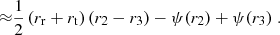
In the last step, we took r2 ≈ rr and r3 ≈ rt, that is, we replaced the radii of the images by the radii of the closest critical curve. Furthermore, 2ry < r2 − r3, meaning that the last term in the second bracket can be omitted. Inserting the result into Eq. (A.1), Eq. (9) is obtained.
Appendix B: Estimated detection rate for supernovae
We assume a given rate of observable multiply imaged SNe per cluster per year for a given source redshift interval, RSN, as detailed in Sect. 4.2. Summing the SNe of all types, RSN = 30 per cluster per year. Subsequently, the detection rate of multiply imaged SNe caused by all clusters with masses between 1.8 and 2.0 × 10¹⁵ M⊙ at redshift zl is given by
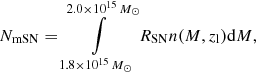
in which n(M, z)dM is the number density of lenses in the mass interval dM as introduced in Sect. 2.2. Using the software described in Murray et al. (2013), we obtain for the number density of lenses in the given mass range
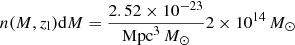
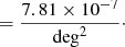
To arrive at this result, we assumed that the cluster extends about 1 Mpc along the line of sight. Multiplying it by RSN, the resulting detection rate of 2.35 × 10⁻⁵ multiply imaged SNe per square degree per year is obtained.
All Tables
Synopsis of observed multiply imaged QSOs with their largest image separation δθ and measured time delays τ.
Results of the comparison between different time-varying, multiply imaged sources behind galaxy clusters.
All Figures
|
Fig. 1. Left panel: distribution of observable FRB host galaxies with total flux above 10 μJy at 1.4 GHz per square degree per redshift, dngal(z)/dz, binned in redshift bins of 0.1 width taken from the SKA Simulated Skies. Middle panel: distribution of potentially observable FRBs from these host galaxies per square degree per year, assuming an internal emission rate of Rint = 10−4 per galaxy per day. Right panel: integrated number of observable FRBs per square degree per year from z to zlim = 6. |
| In the text | |
|
Fig. 2. Left panel: halo-mass function according to Sheth et al. (2001) for z = 0 (solid line) and z = 1 (dashed line). Middle panel: lensing probability according to Eq. (3) for zs from 0.1 to 6.0 and NFW halos with a minimum Einstein radius of 5 arcseconds. Right panel: integrated number of observable multiply imaged FRBs per square degree per year from z = 0 out to zlim from 0.1 to 6.0 according to Eq. (6). |
| In the text | |
|
Fig. 3. Accuracy of the approximation of the time delay: ratio between τ≈, Eq. (12), and τ, Eq. (11), for the two images straddling the radial critical curve in NFW profiles with rs = 0.5 Mpc for κs = 0.15 (dotted curve), κs = 0.2 (solid curve), and κs = 0.3 (dashed curve) vs. the observed angular separation of the two images δθ = (r1 − r2)rs/Dl. |
| In the text | |
|
Fig. 4. Difference between time delays of repeating multiply imaged FRBs for increasing angular distances at the radial critical curve of the NFW profile of Sect. 2.3 when the virial mass of the NFW profile is increased by 105 solar masses (solid line), by 107 solar masses (dashed line), and by 1012 solar masses (dash-dotted line). The measurement precision of τij for one measurement, approximately 1 ms, is shown as a dotted line. |
| In the text | |
|
Fig. 5. Comparison between Grale lens models for the simulated, generalised NFW profile that is detailed in Liesenborgs & De Rijcke (2012). Each map shows the reconstructed critical curves (red, solid lines) and the reconstructed caustics (blue, solid lines) together with the true critical curves (black, dashed lines) for the Grale models with the same constraints detailed in Table 1 and Fig. 7 (i.e. the left and right columns show models without and including an additional mass-sheet basis function, respectively). Top left panel: model includes no additional mass sheet and no timedelay constraints. Top right panel: using an additional mass sheet. Second row, left: including time-delay constraints between the three multiple images marked by the black dots. Second row, right: as in the left-hand side but using an additional mass sheet. Third row, left: including one time-delay constraint between the multiple images marked by the black dots. Third row, right: as in the left-hand side but with an additional mass sheet. Fourth row, left: same as above but for a different pair of multiple images. Fourth row, right: as for the left-hand side but with an additional mass sheet. |
| In the text | |
|
Fig. 6. Comparison between Grale lens models for the simulated, generalised NFW profile that is detailed in Liesenborgs & De Rijcke (2012). Each plot shows the reconstructed convergence values and their uncertainties (black points with error bars) and the true convergence values (blue points) at the positions of the multiple images measured as radial distance from the centre of the NFW profile for the Grale models with the same constraints as detailed in Table 1 and Fig. 5. |
| In the text | |
|
Fig. 7. Comparison between Grale lens models for the simulated, generalised NFW profile that is detailed in Liesenborgs & De Rijcke (2012). Each map shows the difference between the reconstructed convergence map and the simulation result for the models with the same constraints as detailed in Table 1 and Fig. 5. The circles mark the positions of the multiple images and their size is proportional to the difference between the reconstructed and real convergence at these positions. The white circles indicate the multiple images with the time-delay constraints. For the multiple images marked by red circles, no time-delay constraint is given. |
| In the text | |
|
Fig. 8. Left panel: distribution of observable GRB starburst host galaxies with total flux above 10 μJy at 1.4 GHz per square degree, per redshift, dngal(z)/dz, in redshift bins of 0.1 width taken from the SKA Simulated Skies. Middle panel: integrated number of observable GRBs per square degree per year from z to zlim = 6 assuming an internal emission rate of Rint = 10−4 per galaxy per day (solid line) or Rint = 10−5 per galaxy per year (dashed line). Right panel: integrated number of observable multiply imaged GRBs per square degree per year out to zlim from 0.1 to 6.0 according to Eq. (6). |
| In the text | |
Current usage metrics show cumulative count of Article Views (full-text article views including HTML views, PDF and ePub downloads, according to the available data) and Abstracts Views on Vision4Press platform.
Data correspond to usage on the plateform after 2015. The current usage metrics is available 48-96 hours after online publication and is updated daily on week days.
Initial download of the metrics may take a while.