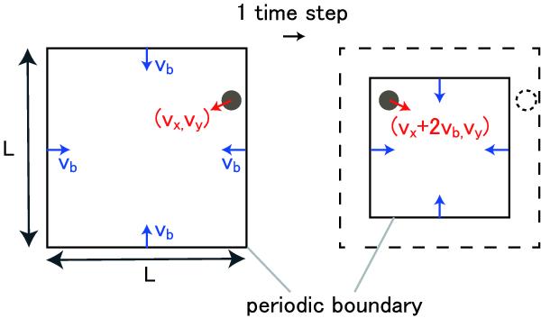
Schematic drawing to illustrate how the particle velocity is calculated when a particle crosses a periodic boundary. For simplicity, we consider this situation in a 2D field, but we actually calculate this in a 3D situation. We consider that a dust particle is close to the boundary in the left figure. In the next time step, the particle crosses the boundary (dashed circle in the right figure). We put the particle on the other side of the boundary as expressed in Eqs. (8) and (10). The velocity component is converted as expressed in Eqs. (9) and (11). This treatment reproduces the isotropic compression in the velocity field well.