A&A 478, 353-369 (2008)
DOI: 10.1051/0004-6361:20078089

Structural properties of disk galaxies

I. The intrinsic equatorial ellipticity of bulges

J. Méndez-Abreu^1,2,4 - J. A. L. Aguerri³ - E. M. Corsini⁴ - E. Simonneau⁵

1 - INAF-Osservatorio Astronomico di Padova, vicolo dell'Osservatorio 5, 35122 Padova, Italy
2 - Universidad de La Laguna, Av. Astrofísico Francisco Sánchez s/n, 38206 La Laguna, Spain
3 - Instituto Astrofísico de Canarias, Calle Vía Láctea s/n, 38200 La Laguna, Spain
4 - Dipartimento di Astronomia, Università di Padova, vicolo dell'Osservatorio 3, 35122 Padova, Italy
5 - Institut d'Astrophysique de Paris, C.N.R.S., 98bis Bd. Arago, 75014 Paris, France

Received 14 June 2007 / Accepted 26 October 2007

Abstract
Context. A variety of formation scenarios have been proposed to explain the diversity of properties observed in bulges. Studying their intrinsic shape can help to constrain the dominant mechanisms at the epochs of their assembly.
Aims. The structural parameters of a magnitude-limited sample of 148 unbarred S0-Sb galaxies were derived in order to study the correlations between bulges and disks, as well as the probability distribution function of the intrinsic equatorial ellipticity of bulges.
Methods. We present a new fitting algorithm (GASP2D) to perform two-dimensional photometric decomposition of the galaxy surface-brightness distribution. This was assumed to be the sum of the contribution of a bulge and disk component characterized by elliptical and concentric isophotes with constant (but possibly different) ellipticity and position angles. Bulge and disk parameters of the sample galaxies were derived from the J-band images, which were available in the Two Micron All Sky Survey. The probability distribution function of the equatorial ellipticity of the bulges was derived from the distribution of the observed ellipticities of bulges and misalignments between bulges and disks.
Results. Strong correlations between the bulge and disk parameters were found. About $80\%$ of bulges in unbarred lenticular and early-to-intermediate spiral galaxies are not oblate but triaxial ellipsoids. Their mean axial ratio in the equatorial plane is $\langle B/A \rangle = 0.85$. Their probability distribution function is not significantly dependent on morphology, light concentration or luminosity. The possible presence of nuclear bars does not influence our results.
Conclusions. The interplay between bulge and disk parameters favors scenarios in which bulges have assembled from mergers and/or have grown over long times through disk secular evolution. However, all these mechanisms have to be tested against the derived distribution of bulge intrinsic ellipticities.

Key words: galaxies: bulges - galaxies: formation - galaxies: fundamental parameters - galaxies: photometry - galaxies: statistics - galaxies: structure

   
1 Introduction

The relative prominence of galactic bulges with respect to their disks is important in the definition of galaxy types. Therefore, understanding the formation of bulges is key to understanding the origin of the Hubble sequence.

Bulges are diverse and heterogeneous (see the reviews by Kormendy & Kennicutt 2004; Wyse et al. 1997; Kormendy 1993). The big bulges of lenticulars and early-type spirals are similar to low-luminosity elliptical galaxies. Their surface-brightness radial profiles generally follow a De Vaucouleurs law (Möllenhoff & Heidt 2001; Andredakis et al. 1995; Carollo et al. 1998, hereafter MH01). The majority of these bulges appear rounder than their associated disks (Kent 1985). Their kinematical properties are well described by dynamical models of rotationally flattened oblate spheroids with little or no anisotropy (Cappellari et al. 2006; Kormendy & Illingworth 1982; Davies & Illingworth 1983). They have photometrical and kinematical properties, which satisfy the fundamental plane (FP) correlation (Bender et al. 1992, 1993; Aguerri et al. 2005a; Burstein et al. 1997). On the contrary, the small bulges of late-type spiral galaxies seems to be reminiscent of disks. Their surface-brightness radial profiles have an almost exponential falloff (de Jong 1996; MacArthur et al. 2003; Andredakis & Sanders 1994). In some cases they have apparent flattenings that are similar or even larger than their associated disks (Fathi & Peletier 2003) and rotate as fast as disks (Kormendy et al. 2002; Kormendy 1993). Late-type bulges deviate from the FP (Carollo 1999).

Different formation mechanisms (or at least a variety of dominant mechanisms at the epochs of star formation and mass assembly) were proposed to explain the variety of properties observed in bulges. Some of these formation processes are rapid. They include early formation from the dissipative collapse of protogalactic gas clouds (Merlin & Chiosi 2006; Sandage 1990; Gilmore & Wyse 1998; Eggen et al. 1962) or later assembly from mergers between pre-existing disks (Baugh et al. 1996; Kauffmann 1996; Cole et al. 2000). In both scenarios the disk forms after the bulge as a consequence of either a long star-formation time compared to the collapse time or a re-accretion around the newly formed bulge.

Bulges can also grow over long timescales through the disk secular evolution driven by bars and/or environmental effects. Bars are present in more than half of disk galaxies in the local universe (Menéndez-Delmestre et al. 2007; Eskridge et al. 2000) and out to $z\sim1$(Jogee et al. 2004; Elmegreen et al. 2004). They are efficient mechanisms for driving gas inward to the galactic center and feed the galactic supermassive black hole (see Corsini et al. 2003a, and references therein). In addition, bar dissolution due to the growth of a central mass (Pfenniger & Norman 1990), scattering of disk stars at vertical resonances (Combes et al. 1990), and coherent bending of the bar perpendicular to the disk plane (Athanassoula 2005; Debattista et al. 2004; Raha et al. 1991; Martinez-Valpuesta et al. 2006) are efficient mechanisms in building central bulge-like structures, the so-called boxy/peanut bulges. Moreover, the growth of the bulge out of disk material may also be externally triggered by satellite accretion during minor merging events (Searle & Zinn 1978; Aguerri et al. 2001; Eliche-Moral et al. 2006) and gas infall (Thakar & Ryden 1998).

Traditionally, the study of the relations between the structural parameters of the galaxies have been used to understand the bulge formation processes, e.g., the correlation between the bulge effective radius and the scale length of the disk in many galaxy samples has always been interpreted as an indication that bulges were formed by secular evolution of their disks (see MacArthur et al. 2003). However, one piece lost in this study is the three-dimensional shape of the bulges. By studying this, one might be able to provide the relative importance of rapid and slow processes in assembling the dense central components of disk galaxies. A statistical study can provide a crucial piece of information for testing the results of numerical simulations of bulge formation for different galaxy type along the morphological sequence.

In this paper, we analyze a sample of unbarred early-type disk galaxies to derive the intrinsic ellipticity of their bulges in the galactic plane. The twisting of bulge isophotes (Lindblad 1956; Zaritsky & Lo 1986) and misalignment between the major axes of the bulge and disk (Bertola et al. 1991) are not possible if the bulge and disk are both oblate. Therefore, they were interpreted as a signature of bulge triaxiality. This idea is supported by the presence of non-circular gas motions (e.g., Bertola et al. 1989; Gerhard & Vietri 1986; Gerhard et al. 1989; Berman 2001) and a velocity gradient along the galaxy minor axis (Corsini et al. 2003b; Coccato et al. 2004, 2005). We improve the previous works in several aspects. First, we use near-infrared images to map the distribution of the mass-carrying evolved stars and avoid contamination of dust and bright young stars. Second, we retrieve the structural parameters of the bulge and disk by applying a new algorithm for two-dimensional photometric decomposition of the observed surface-brightness distribution. Finally, we obtain the probability distribution function (PDF) of the intrinsic equatorial ellipticity of bulges by using a new mathematical treatment of the equations describing their three-dimensional shape.

The paper is organized as follow. The selection criteria of our sample galaxies and the analysis of their near-infrared images are described in Sect. 2. Our new photometric decomposition method for deriving the structural parameters of the bulge and disk by analyzing the two-dimensional surface brightness distribution of galaxies is presented in Sect. 3. The correlations between the structural parameters of the sample galaxies are discussed in Sect. 4. The PDF of intrinsic equatorial ellipticity of the studied bulges is derived in Sect. 5. Our conclusions and a summary of the results are given in Sect. 6.

   
2 Sample selection and data acquisition

Our objective was to select a well-defined complete sample of nearby unbarred disk galaxies to study in a systematic way the photometric properties of their structural components. Since these properties are strongly dependent on the dominating stellar population at the observed wavelength, it is preferable to consider near-infrared images to map the mass-carrying evolved stars and avoid contamination due to dust and bright young stars (e.g., MH01). The complete sample is drawn from the Extended Source Catalogue (XSC) (Jarrett et al. 2000) of the Two Micron All Sky Survey (2MASS) (Skrutskie et al. 2006). Our sample consists of galaxies that meet the following requirements: (1) Hubble type classification from S0 to Sb ( $\rm -3 \leq HT \leq 3$; de Vaucouleurs et al. 1991, hereafter RC3) to ensure that bulges are fully resolved in 2MASS images; (2) unbarred classification in RC3; (3) total J-band magnitude J_T<10 mag (2MASS/XSC); (4) inclination $i<65^{\circ}$ (RC3) to measure the misalignment between the position angle of the bulge and disk; (5) Galactic latitude $\mid$$b_{\rm G}$ $\mid~ > 30^{\circ}$ (RC3) to minimize both Galactic extinction and contamination due to Galactic foreground stars.

We ended up with a sample of 184 bona-fide unbarred galaxies. We retrieved their 2MASS J-band images from the NASA/IPAC Infrared Science Archive. The galaxy images were reduced and flux calibrated with the standard 2MASS extended source processor GALWORKS (Jarrett et al. 2000). Images have a typical field of view of few arcmin and a spatial scale of 1'' pixel^-1. They were obtained with an average seeing ${\it FWHM}\sim3\hbox{$.\!\!^{\prime\prime}$ }1$ as measured by fitting a circular two-dimensional Gaussian to the field stars.

After a visual inspection of the images, we realized that some of the sample galaxies were not suitable for our study. We rejected paired and interacting objects as well as those galaxies that resulted in being barred after performing the photometric decomposition (see Sect. 3). Therefore, the final sample presented in this paper contains 148 galaxies (90 lenticular and 58 early-type spiral galaxies). A compilation of their main properties is given in Table 3. Figure 1 shows the distribution of the sample galaxies over the Hubble types. The lenticular galaxies are predominant over the spirals due to our magnitude selection, which favors red galaxies. Moreover, we show the distribution of radial velocities of the sample galaxies with respect to the 3K background. The mean radial velocity is 2000 km s^-1(corresponding to a distance of 27 Mpc by assuming H₀=75 km s^-1 Mpc^-1), but we include galaxies as far as 8500 km s^-1 (113 Mpc) because the sample is magnitude limited.

Tonry et al. (2001) derived the distance of 30 galaxies of our sample from the measurement of their surface brightness fluctuations. The difference between the distances obtained from radial velocities and those derived from surface brightness fluctuations was calculated for all these galaxies. The standard deviation of the distance differences is 5 Mpc and it was assumed as being a typical distance error. For the 4 common galaxies in the Virgo cluster it is 2 Mpc.

	Figure 1: Distribution of the sample galaxies over the Hubble types ( left panel) and radial velocities with respect to the 3 K background ( right panel).
Open with DEXTER

   
3 Two-dimensional bulge-disk parametric decomposition

Conventional bulge-disk decompositions based on elliptically averaged surface-brightness profiles usually do not take into account the intrinsic shapes (e.g., Prieto et al. 2001) or the position angle (e.g., Trujillo et al. 2001c) of the bulge and disk components, which can produce systematic errors in the results (e.g., Byun & Freeman 1995).

For this reason a number of two-dimensional parametric decomposition techniques have been developed in the last years. As examples we may point out the algorithms developed by Simard (1998, GIM2D), Peng et al. (2002, GALFIT), de Souza et al. (2004, BUDDA) and Pignatelli et al. (2006, GASPHOT). These methods were developed to solve different problems of galaxy decomposition when fitting the two-dimensional galaxy surface-brightness distribution. They use different functions to parametrize the galaxy component and different minimizations routines to perform the fit.

In this paper we present our new decomposition algorithm named GASP2D (GAlaxy Surface Photometry 2 Dimensional Decomposition). The code works like GIM2D and GASPHOT in minimizing the interaction with the user. It works in an automatical way to be more efficient when dealing with a large amount of galaxies. However, like GALFIT and BUDDA it also adopts a Levenberg-Marquardt algorithm to fit the two-dimensional surface-brightness distribution of the galaxy. This reduces the amount of computational time needed to obtain a robust and reliable estimate of the galaxy structural parameters.

In the present work, we show the first version of the code. We assume that the galaxy can be modeled with only two components, the bulge and the disk. In a forthcoming paper, we will show an improved version of GASP2D with the possibility to fit other galaxy components, like bars.

   
3.1 Photometric model

We assumed the galaxy surface-brightness distribution to be the sum of the contribution of a bulge and disk component. Both of them are characterized by elliptical and concentric isophotes with constant (but possibly different) ellipticity and position angles.

Let $(\xi$, $\eta$, $\zeta)$ be the Cartesian coordinates with the origin in the galaxy center, the $\xi$-axis parallel to the direction of right ascension and pointing westward, the $\eta$-axis parallel to the direction of declination and pointing northward, and the $\zeta$-axis along the line-of-sight and pointing toward the observer. The plane of the sky is confined to the $(\xi,~\eta)$ plane.

We adopted the Sérsic law (Sérsic 1968) to describe the surface brightness of the bulge component. The Sérsic law has been extensively used in the literature for modeling the surface brightness profiles of galaxies. For instance, it has been used to model the surface brightness of elliptical galaxies (Graham & Guzmán 2003), bulges of early and late type galaxies (Aguerri et al. 2004; Möllenhoff 2004; Andredakis et al. 1995; Prieto et al. 2001), the low surface brightness host galaxy of blue compact galaxies (Caon et al. 2005; Amorín et al. 2007) and dwarf elliptical galaxies (Graham & Guzmán 2003; Aguerri et al. 2005b; Binggeli & Jerjen 1998). It is given by

$$I_{\rm b}(\xi,\eta)=I_{\rm e}10^{-b_n\left[\left(r_{\rm b}/r_{\rm e} \right)^{1/n}-1\right]},$$ (1)

where $r_{\rm e}$, $I_{\rm e}$, and n are the effective (or half-light) radius, the surface brightness at $r_{\rm e}$, and a shape parameter describing the curvature of the surface-brightness profile, respectively. The value of b_n is coupled to n so that half of the total luminosity of the bulge is within $r_{\rm e}$ and can be approximated as b_n = 0.868 n - 0.142 (Caon et al. 1993). Bulge isophotes are ellipses centered on $(\xi_0,~\eta_0)$ with constant position angle PA$_{\rm b}$ and constant ellipticity $\epsilon_{\rm b} = 1 - q_{\rm b}$. The radius $r_{\rm b}$ is given by

 

$$r_{\rm b} = \left[(-(\xi-\xi_0)\sin{{\rm PA_b}} + (\eta-\eta_0) \... ...)\cos{{\rm PA_b}} + (\eta-\eta_0) \sin{{\rm PA_b}})^2/q_{\rm b}^2\right]^{1/2}.$$ (2)

We adopted the exponential law (Freeman 1970) to describe the surface brightness of the disk component

$$I_{\rm d}(\xi,\eta) = I_0~{\rm e}^{-r_{\rm d}/h},$$ (3)

where I₀ and h are the central surface brightness and scalelength of the disk, respectively. Disk isophotes are ellipses centered on $(\xi_0,~\eta_0)$ with constant position angle PA$_{\rm d}$ and constant ellipticity $\epsilon_{\rm d} = 1 - q_{\rm d}$. Disk inclination is $i = \arccos{(q_{\rm d})}$. The radius $r_{\rm d}$ is given by

 

$$r_{\rm d} = \left[(-(\xi-\xi_0) \sin{{\rm PA_d}} + (\eta-\eta_0) ... ... \cos{{\rm PA_d}} + (\eta-\eta_0) \sin{{\rm PA_d}})^2/q_{\rm d}^2\right]^{1/2}.$$ (4)

To derive the coordinates $(\xi_0,~\eta_0)$ of the galaxy center and the photometric parameters of the bulge ($I_{\rm e}$, $r_{\rm e}$, n, PA$_{\rm b}$, and $q_{\rm b}$) and disk (I₀, h, PA$_{\rm d}$, and $q_{\rm d}$) we fitted iteratively a model of the surface brightness $I_{\rm m}(\xi,~\eta)$= $I_{\rm b}(\xi,~\eta)$+ $I_{\rm d}(\xi,~\eta)$ to the observations using a non-linear least-squares minimization method. It was based on the robust Levenberg-Marquardt method (e.g., Press et al. 1996) implemented by More et al. (1980). The actual computation was done using the MPFIT algorithm implemented by Markwardt under the IDL environment. MPFIT allows the user to keep constant or impose boundary constraints on any parameter during the fitting process.

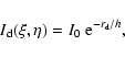
For each pixel $(\xi,~\eta)$, the observed galaxy photon counts $I_{\rm g}(\xi,~\eta)$ are compared with those predicted from the model $I_{\rm m}(\xi,~\eta)$. Each pixel is weighted according to the variance of its total observed photon counts due to the contribution of both galaxy and sky, and determined assuming photon noise limitation by taking into account the detector readout noise (RON). Therefore, the $\chi^2$ to be minimized can be written as

$$\chi^{2} = \sum_{\xi=1}^{N} \sum_{\eta=1}^{M} \frac{[~I_{\r... ...{ I_{\rm g}~(\xi,~\eta) +I_{\rm s}~(\xi,~\eta)+ {\rm RON}^2},$$ (5)

with $\xi$ and $\eta$ ranging over the whole $N \times M$ pixel image.

An important point to consider here is the weight function used to calculate the $\chi^2$; some authors claim that is better to assign to each pixel an uncertainty given by the Poissonian noise (e.g., Peng et al. 2002) while others adopt constant weights to obtain better results (e.g., MH01; de Souza et al. 2004). Both possibilities were implemented in the fitting algorithm. We adopted the Poissonian weights after extensive testing with artificial galaxies.

   
3.2 Seeing effects

The ground-based images are affected by seeing, which scatters the light of the objects and produces a loss of spatial resolution. This is particularly critical in the central regions of galaxies, where the slope of the radial surface brightness profile is steeper. Since the bulge contribution dominates the surface brightness distribution at small radii, seeing mostly affects bulge structural parameters. Seeing effects on the scale parameters of a Sérsic surface brightness profile have been extensively discussed by Trujillo et al. (2001a,b).

During each iteration of the fitting algorithm, the seeing effects were taken into account by convolving the model image with a circular two-dimensional Gaussian point spread function (PSF). The PSF FWHM was chosen to match the one measured from the foreground stars in the field of the 2MASS galaxy image. The convolution was performed in the Fourier domain using the fast Fourier transform (FFT) algorithm (Press et al. 1996) before the $\chi^2$ calculation. Our code allows us to introduce also a Moffat or a star image to reproduce the PSF. We tested that the results are not improved by adopting a circular two-dimensional Moffat PSF or by computing the convolution integrals.

   
3.3 Technical procedure of the fit

Since the fitting algorithm is based on a $\chi^2$ minimization, it is important to adopt initial trials for free parameters as close as possible to their actual values. This would ensure that the iteration procedure does not just stop on a local minimum of the $\chi^2$ distribution. To this aim we proceeded through different steps.

First, the photometric package SExtractor (see Bertin & Arnouts 1996, for details) was used to measure position, magnitude and ellipticity of the sources (e.g., foreground stars, background and companion galaxies, as well as bad pixels) in the images.

We then derived the elliptically-averaged radial profiles of the surface brightness, ellipticity and position angle of the galaxy. We fitted ellipses to the galaxy isophotes with the ELLIPSE task in IRAF. After masking the spurious sources using the parameters provided by SExtractor, we fitted ellipses centered on the position of the galaxy center. This could be estimated by either a visual inspection of the image or with SExtractor. The coordinates of the galaxy center were adopted as initial trials for $(\xi_0,~\eta_0)$ in the two-dimensional fit.

In the third step we derived some of the trial values by performing a standard one dimensional decomposition technique similar to that adopted by several authors (e.g., Kormendy 1977; Prieto et al. 2001). We began by fitting an exponential law to the radial surface-brightness profile at large radii, where the light distribution of the galaxy is expected to be dominated by the disk contribution. The central surface brightness and scalelength of the fitted exponential profile were adopted as initial trials for I₀ and h, respectively. The fitted profile was extrapolated at small radii and then subtracted from the observed radial surface-brightness profile. The residual radial surface-brightness profile was assumed to be a first estimate of the light distribution of the bulge. We fitted it with a Sérsic law by assuming the bulge shape parameter to be 0.5, 1, 1.5,..., 6. The bulge effective radius, effective surface brightness, and shape parameter that (together with the disk parameters) gave the best fit to the radial surface-brightness profile were adopted as initial trials for $r_{\rm e}$, $I_{\rm e}$, and n, respectively.

We also obtained the initial trials for ellipticity and position angle of the disk and bulge, respectively. The values for $q_{\rm d}$ and PA$_{\rm d}$ were found by averaging the values in the outermost portion of the radial profiles of ellipticity and position angle. The initial trials for $q_{\rm b}$ and PA$_{\rm b}$ were estimated by interpolating at $r_{\rm e}$ the radial profiles of the ellipticity and position angle, respectively.

Finally, the initial guesses were adopted to initialize the non-linear least-squares fit to galaxy image, where all the parameters, including n, were allowed to vary. A convergent model was reached when the $\chi^2$ had a minimum and the relative change of the $\chi^2$ between the iterations was less than 10^-7. A model of the galaxy surface-brightness distribution was built using the fitted parameters. It was convolved with the adopted circular two-dimensional Gaussian PSF and subtracted from the observed image to obtain a residual image. In order to ensure the minimum in the $\chi^2$-space found in this first iteration, we perform two more iterations. In these iterations, all the pixels and/or regions of the residual image with values greater or less than a fixed threshold, controlled by the user, were rejected. Those regions were masked out and the fit was repeated assuming, as initial trials for the free parameters, the values obtained in the previous iteration. These kind of masks are usually useful when galaxies have other prominent structures, different from the bulge and disk (e.g. spiral arms and dust lanes), which can affect the fitted parameters, solving the problem in an automatic way. We found that after three iterations the algorithm converges and the parameters do not change.

Table 1: Relative errors on the photometric parameters of the bulge and disk calculated for different galaxy magnitudes by means of Monte Carlo simulations.

   
3.4 Test on simulated galaxies

To test the reliability and accuracy of our two-dimensional technique for bulge-disk decomposition, we carried out extensive simulations on a large set of artificial disk galaxies. We generated 1000 images of galaxies with a Sérsic bulge and an exponential disk. The central surface-brightness, scalelength, and apparent axial ratios of the bulge and disk of the artificial galaxies were randomly chosen in the range of values observed in the J-band by MH01 for a sample of 40 bright spiral galaxies. The adopted ranges were

$$1 \leq r_{\rm e} \leq 3\ {\rm kpc} \qquad 0.4 \leq q_{\rm b} \leq 0.9 \qquad 0.5 \leq n \leq 6\\$$ (6)

for the bulge parameters, and

$$2 \leq h \leq 5\ {\rm kpc} \qquad 0.4 \leq q_{\rm d} \leq 0.9 \\$$ (7)

for the disk parameters. The parameters of the artificial galaxies also have to satisfy the following conditions

$$q_{\rm d} < q_{\rm b} \qquad 0 < B/T < 0.8 \qquad 8 < J_T < 12 \ {\rm mag}.$$ (8)

All the simulated galaxies were assumed to be at a distance of 30 Mpc. This is the average distance of the galaxies of our sample and it corresponds to a scale of 145 pc arcsec^-1. The pixel scale used was 1 arcsec pixel^-1, and the CCD gain and RON were 8 e^- ADU^-1 and 40 e^-, respectively, in order to mimic the instrumental setup of the 2MASS data. Finally, a background level and photon noise were added to the resulting images to yield a signal-to-noise ratio similar to that of the available 2MASS images.

The two-dimensional parametric decomposition was applied to analyze the images of the artificial galaxies as if they were real. Errors on the fitted parameters were estimated by comparing the input $p_{\rm i}$ and output $p_{\rm o}$ values. Relative errors ( $1-p_{\rm i}/p_{\rm o}$) were assumed to be normally distributed, with mean and standard deviation corresponding to the systematic and typical error on the relevant parameter, respectively.

The results of the simulations are given in Table 1. In Run 1 we built the artificial galaxies by assuming the correct values of PSF FWHM and sky level, so only errors due to the Poisson noise are studied. The mean relative errors on the fitted parameters are smaller than 0.01 (absolute value) and their standard deviations are smaller than 0.02 (absolute value) for all galaxies with J_T<10 mag, proving the reliability of our derived structural parameters. Relative errors increase for fainter galaxies, which are not included in our sample.

Systematic errors given by a wrong estimation of PSF and sky level are the most significant contributors to the error budget. To understand how a typical error in the measurement of the PSF FWHM affects our results, we analyzed the artificial galaxies by adopting the correct sky level and a PSF FWHM that was $2\%$larger (Run 2) or smaller (Run 3) than the actual one. As expected (Sect. 3.2), the parameters of the surface-brightness profiles show larger errors for the bulge than for the disk. We recovered larger values for the Sérsic parameters ($r_{\rm e}$, n) when the PSF FWHM is overestimated, and lower values when it is underestimated. Relative errors are correlated with the values of effective radius and shape parameter of the bulge but not with the magnitude of the galaxy. In Run 4 we built the artificial galaxies by adopting the correct PSF FWHM and a sky level that was $1\%$ larger than the actual one. For brighter galaxies an improper sky subtraction mostly affects the parameters of the disk surface-brightness profile. For fainter galaxies, the large relative errors on the bulge parameters are due to their coupling with the disk parameters. This is consistent with the results of similar tests performed by Byun & Freeman (1995).

The structural parameters to be measured to derive the intrinsic shape of bulges are the ellipticity of the bulge and position angles of the bulge and disk (Sect. 5.2). In all the runs, the relative errors are smaller than 0.05 (absolute value) for galaxies with J_T<10 mag. Larger errors ( up to about 0.1) were found for fainter galaxies after an improper subtraction of the sky level from the image. However, this is not the case for our sample galaxies.

   
3.5 Results and comparison with previous studies

The parameters derived for the structural components of the sample galaxies are collected in Table 3. All the listed values are corrected for seeing smearing and galaxy inclination. Surface brightnesses were calibrated by adopting, for the 2MASS images, the flux zero point given in the image headers (Jarrett et al. 2000).

The comparison of the structural parameters obtained for the same galaxy by different authors is often not straightforward on account of possible differences in the observed bandpass, parameterization of the surface-brightness distribution, and fitting method.

MH01 already studied 11 of our sample galaxies (NGC 772, NGC 2775, NGC 2841, NGC 2985, NGC 3169, NGC 3626, NGC 3675, NGC 3898, NGC 4450, NGC 4501 and NGC 4826). They performed a two-dimensional parametric decomposition of the J-band surface brightness distribution. They considered ellipticities and position angles of both the bulge and disk as free parameters. Therefore, we considered their results as the most suitable to be compared with ours. The structural parameters we measured are consistent with those given by MH01, within $25\%$ for all the common galaxies but NGC 4826. We argue that they strongly underestimated the scale length of its disk (and consequently obtained a wrong estimate of the other parameters) because of the small field of view ( $3'\times3'$) of their image. In Fig. 2 we show the comparison between our axial ratios and position angles of the bulge and disk and those measured by MH01.

	Figure 2: Comparison between the axis ratios ( left panel) and the position angles ( right panel) measured in this paper and by MH01. Filled dots and open diamonds correspond to values measured for bulges and disks, respectively. Residuals $\Delta q$ and $\rm\Delta PA$ are defined as $1 - q_{\rm ~ MH01}/q_{\rm our}$ and $\rm 1 - PA_{\rm MH01}/PA_{\rm our}$, respectively.
Open with DEXTER

   
4 Correlations between structural parameters

The study of correlations between the structural parameters of bulges and disks of our sample galaxies will help us to both cross check our results with those available in literature and identify and rule out peculiar bulges from any further analysis.

   
4.1 Bulge parameters

We did not find any correlations between the bulge parameters and Hubble type. Neither the effective radius (Fig. 3A), effective surface brightness (Fig. 3B) nor the n shape parameter (Fig. 3C) show a statistically significant Pearson correlation coefficient (r).

From near-infrared observations of spiral galaxies, Andredakis et al. (1995) found that bulges of early-type spirals are characterized by $n\approx4$ (i.e., they have a de Vaucouleurs radial surface brightness profile), while the bulges of late-type spirals are characterized by $n\approx1$ (i.e., they have an exponential radial surface brightness profile). This early result was confirmed in various studies (e.g., de Jong et al. 1996; Khosroshahi et al. 2000; MacArthur et al. 2003; MH01; Möllenhoff 2004; Hunt et al. 2004). We argue that our data does not show such a correlation due to the smaller range of Hubble types covered by our sample (S0-Sb) with respect to the cited works, where it is mostly evident for Hubble types later than Sb.

Figure 3: Correlations between the bulge parameters. Correlation between the Hubble type and effective radius (A), effective surface brightness (B), and shape parameter (C). Correlations between the effective radius and shape parameter (D), effective surface brightness (E), and absolute magnitude (F). In each panel the solid line represent the linear regression through all the points. The Pearson correlation coefficient (r), and the results of the linear fit (y =a + bx) are also given.

Open with DEXTER

The n shape parameter increases with effective radius. Larger bulges have a surface-brightness radial profile that which is more centrally peaked than that of the smaller bulges (Fig. 3D). We obtained

$$\log n = 0.38 (\pm 0.02) + 0.18 (\pm 0.05)~\log r_{\rm e}\ \qquad (r = 0.28).$$ (9)

The effective surface brightness is dependent on the effective radius. Larger bulges have a lower effective surface brightness (Fig. 3E). We found a linear regression

$$\log \mu_{\rm e} = 17.74 (\pm 0.07) + 1.7 (\pm 0.2)~\log r_{\rm e}\ \qquad (r = 0.55).$$ (10)

This is in agreement, within the errors, with the correlation by MH01. If we use the mean surface brightness inside one effective radius instead of the effective surface brightness this relation becomes the so-called Kormendy relation, already known for bulges and elliptical galaxies (Kormendy 1977).

Finally, the absolute luminosity of the bulge is correlated with the effective radius. Larger bulges are more luminous (Fig. 3F). This result in

$$M_{\rm b} = -21.93 (\pm 0.06) - 3.4 (\pm 0.2)~\log r_{\rm e}\ \qquad (r = -0.80),$$ (11)

where $M_{\rm b}$ is the J-band magnitude of the bulge. A similar result was obtained by MH01 for a smaller sample of disk galaxies spanning a larger range of Hubble types.

Bulges and elliptical galaxies follow a tight relation, the FP, defined by the effective radius, mean surface brightness within effective radius, and central velocity dispersion (Dressler et al. 1987; Djorgovski & Davis 1987). Therefore, we derived the FP for the bulges of our sample galaxies. The measurements of the central stellar velocity dispersion for a subsample of 98 galaxies were available in literature and were retrieved from the on line HyperLeda catalog (Paturel et al. 2003). The velocity dispersions given by the catalogue are corrected to a circular aperture of radius of 0.595 h^-1 kpc, which is equivalent to an angular diameter of $3\hbox{$.\!\!^{\prime\prime}$ }4$ at the distance of Coma, following the prescription by Jorgensen et al. (1995). The aperture-corrected velocity dispersions are given in Table 3. The coefficients describing the FP

$$\log r_{\rm e}\!=\!1.08 (\pm 0.09) \log \sigma_0 \!+\! 0.25 (\pm 0.02) \langle \mu_{\rm e} \rangle - 6.61 (\pm 0.40),~$$ (12)

were derived by minimizing the square root of the residuals along the $\log r_{\rm e}$ axis. Errors given for every coefficient were calculated by performing a bootstrap analysis with 1000 iterations. No statistically significant difference was observed when only bulges of lenticular or early-to-intermediate spiral galaxies were considered. The dispersion around this relation is $\sigma=0.11$ dex and was measured as the rms scatter in the residuals of $\log r_{\rm e}$. The observational error on the FP is 0.066 dex and includes the measurement errors in $\log r_{\rm e}$ (0.055 dex), $\log \sigma_0$(0.029 dex), and $\langle \mu_{\rm e} \rangle$ (0.021 mag arcsec^-2). Errors in $\log r_{\rm e}$ and $\langle \mu_{\rm e} \rangle$ are not independent (Kormendy 1977). Compared with the dispersion around the relation, this gives an intrinsic scatter of 0.088 dex. Figure 4 shows an edge-on view of the FP. Our coefficients and those by Falcón-Barroso et al. (2002) are consistent within the errors, although they analyzed K-band data. Unfortunately, we have not found in the literature the coefficient of the FP in the J-band for a direct comparison (see Bernardi et al. 2003).

One of the projections of the FP is the so-called Faber-Jackson relation (FJ), which relates the luminosity of elliptical galaxies and bulges to their central velocity dispersion (Faber & Jackson 1976). We derived the J-band FJ relation for the bulge subsample obtaining

$$\log \sigma_0 = 0.1 (\pm 0.2) - 0.095 (\pm 0.009) M_{\rm b}\ \qquad (r = -0.71).$$ (13)

This result also holds when we consider only galaxies with errors on the central velocity dispersion lower than 10 km s^-1 ( $\Delta\! \log \sigma_0<0.018$ dex). In fact, we derived

$$\log \sigma_0 = 0.4 (\pm 0.3) - 0.085 (\pm 0.013) M_{\rm b}\ \qquad (r = -0.65),$$ (14)

which is consistent within errors with Eq. (13). From Eq. (13) we derived $L \propto \sigma_0^{4.2}$, which is very close to the virial relation and indicates that our bulges share important characteristics with bright elliptical galaxies Matkovic & Guzmán (2005). On the other hand, Balcells et al. (2007) found $L \propto \sigma_0^{2.9}$ (close to faint ellipticals) observing a sample of bulges with the Hubble Space Telescope in the K-band. This discrepancy is not due to the adopted fitting method and it is not observed if only bright bulges ( $M_{\rm b}<-20$ mag) are considered. Indeed, we found $L \propto \sigma_0^{(3.9\pm0.4)}$ for our sample and $L \propto \sigma_0^{(3.6\pm0.7)}$ for the sample by Balcells et al. (2007). The different behaviour of faint bulges ( $M_{\rm b}>-20$ mag) requires further investigation to be explained.

	Figure 4: Edge-on view of the FP for the 98 early-to-intermediate type bulges of our sample with measured velocity dispersion. The solid line represents the linear fit to the data. The dotted lines represent the $1\sigma$ deviation from the fit. The error bars in the lower right corner of the panel indicate the mean errors of the data.
Open with DEXTER

	Figure 5: FJ relation for the 98 early-to-intermediate type bulges of our sample with measured velocity dispersion. The solid line represents the linear fit to the data. The dotted lines represent the $1\sigma$ deviation from the fit. The error bars in the lower right corner of the panel indicate the mean errors of the data.
Open with DEXTER

Khosroshahi et al. (2000) noticed that the shape parameter, effective radius and central surface brightness of elliptical galaxies and bulges are correlated. This relation was termed photometric plane (PP). Figure 6 shows an edge-on view of the PP of our bulge sample

$$\log n \!=\! 0.17 (\pm 0.02) \log r_{\rm e} - 0.088 (\pm 0.004) \mu_0 + 1.48 (\pm 0.05). ~$$ (15)

The coefficients were derived by minimizing the square root of the residuals along the $\log n$ axis. Errors given for every coefficient were calculated by performing a bootstrap analysis with 1000 iterations. No statistically significant difference was observed when only bulges of lenticular or early-to-intermediate spiral galaxies were considered. The dispersion around this relation is $\sigma = 0.04$ and was measured as the rms scatter in the residuals of $\log n$. Our coefficients and those by MH01 are consistent within the errors, although their sample is dominated by bulges of late-type spirals. The presence of the bulges of lenticular and spirals on the same PP hints towards a common formation scenario.

	Figure 6: Edge-on view of the PP for early-to-intermediate bulges of our sample. The solid line represents the linear fit to the data. The dotted lines represent the $1\sigma$ deviation from the fit. The error bars in the lower right corner of the panel indicate the mean errors of the data.
Open with DEXTER

   
4.2 Disk parameters

Regarding the disk parameters, we found no correlation between the scale length and Hubble type (r = -0.06, Fig. 7A). The same is true for the central surface brightness. In fact, it shows a large scatter also with Hubble type (r = -0.05, Fig. 7B). This is consistent with the results of de Jong et al. (1996) and MH01.

On the other hand, the central surface brightness and the luminosity of the disks are dependent on the scale length. Larger disks have a lower central surface brightness (Fig. 7D). We found a linear regression

$$\log \mu_{\rm0} = 17.36 (\pm 0.1) + 1.4 (\pm 0.2)~\log h\ \qquad (r = 0.49),$$ (16)

and brighter disks show larger scale lengths (Fig. 7C)

$$M_{\rm d} = -21.21 (\pm 0.09) - 3.5 (\pm 0.2)~\log h\ \qquad (r = -0.80),$$ (17)

where $M_{\rm d}$ is the J-band magnitude of the disk.

The coefficients are in agreement within the errors with those given by MH01.

	Figure 7: Correlations between the disk parameters. Correlations between the Hubble type and disk scale length (A) and central surface brightness (B). Correlation between the disk scale length and absolute luminosity (C) and central surface brightness (D). Solid lines and coefficients as in Fig. 3.
Open with DEXTER

   
4.3 Bulge and disk interplay

Figure 8: (A) Correlation between the disk scale length and central velocity dispersion for the 98 galaxies of our sample with a measured velocity dispersion. (B) Correlation between the disk scale length and bulge effective radius. (C) The ratio between the bulge and disk exponential scale lengths as a function of the bulge shape parameter. Filled circles and crosses represent the results of our measurements and simulations by Tissera et al. (2006), respectively. Solid lines and coefficients as in Fig. 3.

Open with DEXTER

We have found that the disk scale length increases with central velocity dispersion. Since central velocity dispersion correlates with the virial mass of the bulge ( ${\cal M}_{\rm b} = \alpha r_{\rm e} \sigma_0^2/G$ with $\alpha =5$, Cappellari et al. 2006), we conclude that larger disks are located in galaxies with more massive bulges (Fig. 8A). For the subsample of 98 early-to-intermediate bulges with a measured velocity dispersion we found

$$\log \sigma_0 = 2.13 (\pm 0.03) + 0.27 (\pm 0.06)~\log h\ \qquad (r = 0.42).$$ (18)

We also found a strong correlation between the bulge effective radius and the disk scale length. Larger bulges reside in larger disks (Fig. 8B). This relation was already observed by Courteau et al. (1996) and later observed in NIR by MH01, MacArthur et al. (2003). We obtained a linear regression

$$\log r_{\rm e} = -0.45 (\pm 0.03) + 0.91 (\pm 0.07)~\log h \qquad (r = 0.74),$$ (19)

which is in agreement within error bars with the correlation found by MH01. All these correlations between bulge and disk parameters indicate a link between the bulge and disk formation and evolution history. This connection was interpreted as an indication of the formation of late-type bulges via secular evolution of the disks (Courteau et al. 1996). However, our measurements of the scale lengths of the bulge and disk and n (Fig. 8C) are also fully consistent with the predictions of the numerical simulations by Scannapieco & Tissera (2003) and Tissera et al. (2006). They studied the effects of mergers on the mass distribution of bulges and disks of galaxies formed in hierarchical clustering scenarios. Our mean value $\langle r_{\rm e}/h\rangle=0.36 \pm 0.17$ is also in good agreement with $r_{\rm e}/h$ found by Naab & Trujillo (2006) for a series of major mergers' remnants. These results indicate that these relations are not enough to distinguish between bulges formed by mergers or by secular evolution of the disk, even if a strong crosstalk between both components is present.

   
5 The equatorial intrinsic ellipticity of bulges

In the previous section, we realized that the knowledge of correlations between structural parameters of the bulge and disk is not sufficient to distinguish between the different scenarios that were proposed to explain the formation of bulges. Therefore, we decided to study the intrinsic shape of bulges in order to give a further constraint to these scenarios.

Independently of its internal structure, we can consider a bulge of a spiral galaxy as an ellipsoidal stellar system located in the center of the galaxy, which stands out against the disk in the photometric observations. We assume that both the bulge and disk share the same center, which coincides with the galactic one, and they have the same polar axis (i.e., the equatorial plane of disk coincides with that of bulge).

   
5.1 Geometrical formalism

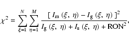
Let (x,y,z) be Cartesian coordinates with the origin in the galaxy center, the x-axis and y-axis corresponding to the principal axes of the bulge equatorial ellipse, and the z-axis corresponding to the polar axis. As the equatorial plane of the bulge coincides with the equatorial plane of the disk, the z-axis is also the polar axis of the disk. If A, B, and C are lengths of the ellipsoid semi-axes, the corresponding equation of the bulge in its own reference system is given by

$$\frac{x^2}{A^2} + \frac{y^2}{B^2} + \frac{z^2}{C^2} = 1.$$ (20)

Let (x',y',z') be now the Cartesian coordinates of the observer system. It has its origin in the galaxy center, the polar z'-axis along the line-of-sight (LOS) and pointing toward the galaxy, and the plane of the sky lies on the (x',y') plane.

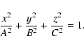
The projection of the disk onto the sky plane is an ellipse whose major axis is the line of nodes (LON), i.e., the intersection between the galactic and the sky planes. The angle $\theta$ between the z-axis and z'-axis corresponds to the inclination of the bulge ellipsoid; it can be derived as $\theta=\arccos{(d/c)}$ from the length c and d of the two semi-axes of the projected ellipse of the disk. We defined $\phi$ ( $0 \leq \phi \leq \pi /2$) as the angle between the x-axis and the LON on the equatorial plane of the bulge (x,y). Finally, we also defined $\psi$ ( $0 \leq \psi \leq \pi /2$) as the angle between the x'-axis and the LON on the sky plane (x',y'). The three angles $\theta$, $\phi$, and $\psi$ are the usual Euler angles and relate the reference system (x,y,z) of the ellipsoid with that (x',y',z') of the observer by means of three rotations. Indeed, since the location of the LON is known, we can choose the x'-axis along it, and consequently it holds that $\psi=0$. By applying these two rotations to Eq. (20) it is possible to derive the equation of the ellipsoidal bulge in the reference system of the observer, as well as the equation of the ellipse corresponding to its projection on the sky plane (Simonneau et al. 1998). Now, if we identify this ellipse with the ellipse that forms the observed ellipsoidal bulge, we can determine the corresponding axes of symmetry $x_{\rm e}$ and $y_{\rm e}$. The first one, on which we measured the semi-axis a, forms an angle $\delta$ with the LON (the x'-axis in the observed plane); the semi-axis b is taken over the $y_{\rm e}$-axis. We always choose $0 \le \delta \le \pi/2$, so it is possible that a either be the major or the minor semi-axis, and vice versa for b.

We have

   

$$a^{2}b^{2} = A^{2}C^{2}\sin^{2}\theta \cos^{2}\phi + B^{2}C^{2}\sin^{2}\theta \sin^{2}\phi + A^{2}B^{2}\cos^{2}\theta.$$ (21)

$$a^{2}+b^{2}=A^{2}(\cos^{2}\phi + \cos^{2}\theta \sin^{2}\phi) + B^{2}(\sin^{2}\phi + \cos^{2}\theta \cos^{2}\phi)$$

$$\quad\quad+ C^{2}\sin^{2}\theta.$$ (22)

$$\tan2\delta\!=\!\frac{(B^{2}-A^{2})\cos\theta\sin2\phi}{A^{2}(\co... ...\! B^{2}(\cos^{2}\theta\cos^{2}\phi - \sin^{2})\! +\! C^{2}\sin^{2}\theta}\cdot$$ (23)

If the ellipsoidal bulge is triaxial ( $A \ne B \ne C$) then it is possible to observe a twist ( $\delta\ne0$; see Eq. (23)) between the axes of the projected ellipses of the bulge and the disk.

   
5.2 Inverse problem or deprojection

We will now focus our attention on the inverse problem, i.e., deprojection. Following Simonneau et al. (1998), from Eqs. (21), (22), and (23), we are able to express the length of the bulge semi-axes (i.e. A, B, and C) as a function of the length of the semi-axes (i.e. a, b) of the projected ellipse and the position angle ($\delta$).

   

$$\frac{a^2+b^2}{2}\left[ 1 + e\left( \cos2\delta + \sin2\delta\frac{\sin\phi}{\cos\phi}\frac{1}{\cos\theta}\right)\right]$$                                    A² = (24)

$$\frac{a^2+b^2}{2}\left[ 1 + e\left( \cos2\delta - \sin2\delta\frac{\cos \phi}{\sin \phi}\frac{1}{\cos\theta}\right)\right]$$ B² = (25)

$$\frac{a^2+b^2}{2}\left[ 1 + e\left( 2\sin2\delta \frac{\cos\theta... ...}{\sin2\phi} - \cos2\delta\frac{1 + \cos^2\theta}{\sin^2\theta} \right)\right],$$ C² = (26)

where e=(a² - b²)/(a² + b²) is, in some way, a measure of the ellipticity. It will be $-1 \le e \le 1$.

Notice that a, b, $\delta$ and $\theta$ are all observed variables. Unfortunately, the relation between the intrinsic and projected variables also depends on the spatial position of the bulge (i.e., on the $\phi$ angle), which is not directly accessible to observations. For this reason, only a statistical determination can be performed to assess the intrinsic shape of bulges.

As A and B are the semi-axis of the equatorial ellipse of the bulge, we have to distinguish between two cases, according to Eqs. (24) and (25). If a>b (or equivalently e>0) then A>B. Otherwise, if a<b (or equivalently e<0) then A<B. Thus, if $\delta \neq 0$ the equatorial plane of the bulge ellipsoid is not circular and the bulge ellipsoid is triaxial.

From Eqs. (24), (25) and (26) we can write the axial ratios A/C and B/C as explicit functions of $\phi$. Moreover, we assume that the angle $\phi$ is random and independent of the length of ellipsoid semi-axes. Thus, the normalized probability distribution $P(\phi)$ of getting a given value of $\phi$ in $(\phi,\phi$+$d\phi)$ is

$$P(\phi)=2/\pi; \qquad \int_{0}^{\pi/2} P(\phi) {\rm d}\phi = 1.$$ (27)

According to a fundamental theorem of statistics, the probability of obtaining a given value of any function $f(\phi)$ (e.g., one of the axial ratios) will be equal to the probability of getting the corresponding value of $\phi$, provided that the ratio d $f/{\rm d}\phi$between the corresponding differential elements is taken into account.

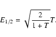
In this work, we will focus our attention on the intrinsic equatorial ellipticity of bulges. We define it as E=(A²-B²)/(A²+B²) with -1<E< 1. In a forthcoming paper, we will study the intrinsic flattening of the bulge ellipsoids defined as the ratio between the length C of polar semi-axis and the mean length of the equatorial semi-axes.

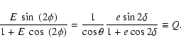
From Eqs. (24) and (25), it is straightforward to derive a relation among the intrinsic variables (equatorial ellipticity E and position angle $\phi$), and the measured (i.e. $\theta$, e, and $\delta$), which is

$$\frac{E~ \sin~(2\phi)}{1 + E~ \cos~(2\phi)} = \frac{1}{\cos\theta}\frac{e\sin2\delta}{1 + e\cos2\delta} \equiv Q.$$ (28)

The second member of the equality in Eq. (28) allows us to define the observable Q in terms of the measured variables $\theta$, e, and $\delta$. It must be stressed that for each specific bulge the relation between the equatorial ellipticity E and the unknown parameter $\phi$ embraces the whole of the measured variables through the single variable Q.

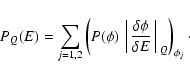
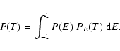
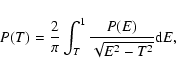
On the one hand, Eq. (28) will yield the conditional probability P_Q(E) that a given bulge, with a measured value of Q, takes on any particular value of E (individual statistic); on the other hand, this equation will give the probability P_E(Q)associated to each value of Q for a bulge with intrinsic equatorial ellipticity E. This latter probability will be the kernel of an integral equation that relates the observed statistical distribution P(Q), corresponding to a sample of galaxies, with the statistical distribution of the equatorial ellipticity P(E) for the same sample.

   
5.3 Individual statistics

For a given galaxy, we can measure the values of $\theta$, e and $\delta$, and then derive the value of Q through Eq. (28). We want to determine the probability P_Q(E) that such a galaxy (i.e. with such a value of Q) will take on a value of Ein the range $(E, E+{\rm d}E)$. The subindex Q specifies this galaxy. All the galaxies with the same value of Q shall partake the same probability distribution P_Q(E).

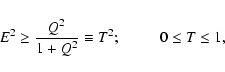
Once the value of Q is prescribed, for some values of E there are not values of $\phi$ ( $0 \le \phi \le \pi/2$) that satisfy Eq. (28). Hence, it shall hold that P_Q(E)=0. Only for those values of E such that

$$E^{2} \ge \frac{Q^2}{1 + Q^2} \equiv T^{2} ;\ \ \qquad 0 \le T \le 1,$$ (29)

will there exist two values of $\phi$ that fulfill Eq. (28).

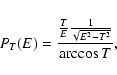
Then for any value of E > T the probability P_Q(E) will be given by

$$P_{Q}(E)=\sum_{j=1,2} \left(P(\phi) \left\arrowvert \frac{\delta \phi}{\delta E} \right\arrowvert_{Q}\right)_{\phi_{j}}\cdot$$ (30)

By calculating the partial derivative of Eq. (30) and normalizing we obtain

$$P_{T}(E)= \frac{\frac{T}{E}\frac{1}{\sqrt{E^{2}-T^{2}}}}{\arccos T},$$ (31)

where the subindex T plays the same role as the subindex Q; both are related through Eq. (29).

This means that the possible values of E are very concentrated and slightly larger than T. To get an idea of how P_T(E) is peaked near the value of T, we calculated the value E_1/2 for which the total probability that E > E_1/2 is equal to the probability that E < E_1/2. For every bulge E_1/2 is a sort of mean value of E, and is given by

$$E_{1/2}=\sqrt{\frac{2}{1+T}}T.$$ (32)

In Fig. 9 we show, as an example, the probability P_T(E) for one galaxy of our sample.

	Figure 9: Probability distribution function of E for the galaxy IC 4310. The dotted line represents the value of T=0.098 derived for this galaxy. The value of E1/2 is also shown in the plot.
Open with DEXTER

   
5.4 Global statistics

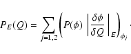
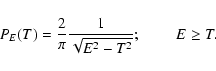
Likewise, we can define the probability P_E(Q) associated to each value of Q for a given bulge of intrinsic equatorial ellipticity E.

For a prescribed value of E, it will only be possible to get the values of $\phi$ that satisfy Eq. (28) when $T \le E$. The probability $P(\phi_{j})$ for the two values of $\phi_j$ is given by Eq. (27). The probability P_E(T) is equal to the sum of the two probabilities $P(\phi_{j})$, weighted with the ratio $(\delta \phi/\delta T)_{E}$ of the differential elements:

$$P_{E}(Q)=\sum_{j=1,2} \left(P(\phi) \left\arrowvert \frac{\de... ... \phi}{\delta Q} \right\arrowvert_{E}\right) _{\phi_{j}}\cdot$$ (33)

Once the partial derivative from Eq. (28) is computed, we obtain

$$P_{E}(T)= \frac{2}{\pi}\frac{1}{\sqrt{E^{2}-T^{2}}};\ \qquad E \ge T .$$ (34)

Our purpose here is to determine the probability distribution P(E), that is the number of galaxies with a value of E inside the interval $(E, E+{\rm d}E)$, starting from a sample that is sufficiently representative. We have measured for such a sample the distribution P(T), namely the number of bulges whose values of T are within Tand $T+{\rm d}T$. We must write now P(T) as the integral over all the values of E of the product of the conditional probability P_E(T)by the so far unknown distribution P(E):

$$P(T)=\int_{-1}^{1}P(E)~P_{E}(T)~{\rm d}E.$$ (35)

Then, by making use of Eq. (34), we obtain an Abel-like integral equation

$$P(T)=\frac{2}{\pi}\int_{T}^{1}\frac{P(E)}{\sqrt{E^2 - T^2}}{\rm d}E,$$ (36)

which will allow us to derive P(E) from the observed distribution P(T).

However, as usual, the data P(T) of our statistical problem takes the form of histograms, hence, the relevant equations must be formulated accordingly.

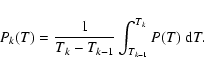
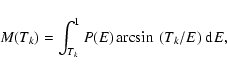
Let T_k with k=0, 1, 2, ..., N (T₀=0, T_N=1) be a set of discrete ordinates that defines the histogram of the observed function P(T) (Fig. 10). The kth-element of this histogram is defined by

$$P_{k}(T)=\frac{1}{T_{k}-T_{k-1}}\int_{T_{k-1}}^{T_{k}}P(T)~{\rm d}T.$$ (37)

We must now seek the integral equation that relates the variables P_k(T) with the probability distribution P(E).

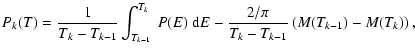
We notice that the integral of P(T) in Eq. (37) is equivalent to the difference between the two quadratures of P(T)over the intervals (T_k-1,1) and (T_k,1). In both of them, we will replace P(T) by its integral form, given by Eq. (36).

Then, by inverting the order of integration, we can easily rewrite the two resulting integrals to obtain

 

$$P_{k}(T)=\frac{1}{T_k -T_{k-1}}\int_{T_{k-1}}^{T_k}~P(E)~{\rm d}E - \frac{2/\pi}{T_{k}-T_{k-1}} \left(M(T_{k-1}) - M(T_{k}) \right),$$ (38)

where we defined

$$M(T_{k})=\int_{T_{k}}^{1}P(E)\arcsin~ (T_k/E) ~{\rm d}E,$$ (39)

and M(T_k-1) in a similar way.

Equation (38) is the integral equation that will allow us to obtain the values of P(E). Since it is consistent with the numerical structure of the data, we are confident that we have eliminated most of the numerical problems that arise from the direct inversion of Eq. (36), which constitutes a typical ill-posed problem.

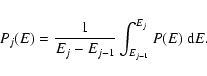
At this point, we require for P(E) the same histogram representation that we have already introduced for the data P(T). We introduce a similar set of discrete ordinates for the variable E (i.e. $E_k \sim T_k$), and an analogous definition to obtain the elements P_k(E) of the histogram

$$P_{j}(E)=\frac{1}{E_{j}-E_{j-1}}\int_{E_{j-1}}^{E_{j}}P(E)~{\rm d}E.$$ (40)

Thus Eq. (38) can be rewritten into the form

$$P_{k}(T)=P_{k}(E) - \frac{2/\pi}{T_{k}-T_{k-1}} \left(M(T_{k-1}) - M(T_{k}) \right).$$ (41)

In order to express the integrals M(T_k-1) and M(T_k) as linear functions of the so far unknown values of P_j(E) (where j > k-1), we consider that P(E) is constant and equal to the unknown values of P_j(E) over each interval (E_j-1, E_j), according to its histogram representation. Therefore, it is straightforward to compute the coefficients CM (k, j), defined by the linear relation

$$M(T_{k})=\sum_{j=k+1}^{N} CM(k,j)~ P_{j}(E).$$ (42)

Thus Eq. (41) becomes a simple linear algebraical equation that relates the terms of the two histograms P_k(T) and P_j(E) through a triangular matrix. Once we have the integral Eq. (36) into a suitable matrix form, according to the histogram representation of the data and results, a simple matrix inversion could be, in principle, enough to obtain the resulting P_j(E). However, such a procedure may add to the intrinsic difficulties, due to the lack of precision typical of the observational data, which naturally arise in the matrix inversion process; a catastrophic mixture when dealing with an inverse problem.

   
5.5 Inversion methods for the integral equation

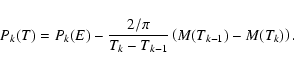
We have considered two different approaches to tackle the numerical problem. The first one is suggested by the method that leads us to the integral Eq. (41) for the set of discrete elements P_k(T). We notice that there are two different terms in its right-hand side. The first one is the identity operator. The second one is the difference between two integrals of P(T), multiplied by a kernel that is quickly decreasing. We can consider the former as the leading term, and treat the latter as a corrective term in a iterative perturbation method. Consequently, we can write Eq. (41) as

$$P_{k}(E)=P_{k}(T) + \frac{2/\pi}{T_{k}-T_{k-1}} \left(M(T_{k-1}) - M(T_{k}) \right),$$ (43)

where we can determine P_kⁱ(E) at the ith-iteration making use of the form of P_k^i-1(E) from the (i-1)th-iteration to compute the correction term [M(T_k-1) - M(T_k)]. As an initial guess, we consider P_k(E) equal to P_k(T) at a zero-order approximation. This iterative process is repeated until convergence is achieved.

From the data P(T) of the histogram shown in Fig. 10, we have obtained a satisfactory solution P(E) with a few number (5-10) of iterations. We will discuss later the physical quality of this solution, but we must recognize here the stability of the method. Actually, we have always achieved the same solution with a few number of iterations, starting from any trial initial distribution (namely, any zero-order approximation for P_k(E)). Moreover, the greater advantage of solving the integral equation by means of an iterative perturbation method is the possibility to recover, according to Eq. (41), the approximate diagram P_kⁱ(T) that corresponds to any iterative solution P_kⁱ(E), and this yields a double check on the evolution and quality of results.

However, when dealing with this kind of inverse problem, it may often happen in the practice that the results are correct mathematically, but not from the physical standpoint. In view of this difficulty, and in spite of the excellent quality of the foregoing iterative method, we wished to develop an alternative method of inversion for the integral Eq. (36), in order to double check the results.

The other way to numerically treat the integral Eq. (36) comes from the analytical inversion

$$\int_{T'}^{1}P(E)=\int_{T'}^{1}\frac{T}{\sqrt{T^{2} - T'^{2}}}~P(T)~{\rm d}T'.$$ (44)

Once we have this analytical form for the required solution, we rewrite it for the histogram representation of P(E), by defining P_k(E) as P_k(T) in Eq. (40). Again the difference between the two integrals of P(T) show up. Now, we impose the histogram model of this P(T) to derive analytically the matrix elements that relate any P_k(E) to all the elements P_k(T). The corresponding solutions obtained with the two methods are the same, allowing for the small differences due to round-off errors of the two different numerical algorithms employed.

Now that we are confident of the reliability of both methods of inversion of the integral equation, we can came back to the aforesaid difficulties.

	Figure 10: PDF of T. The probability is normalized over 10 bins, which are geometrically distributed to cover the interval (0,1). The width of the first bin is 0.03 and the width ratio of two consecutive bins is 1.25. Error bars correspond to Poisson statistics.
Open with DEXTER

When applying either method to the observed distribution P(T), in form of a histogram with bins P_k(T) as shown in Fig. 10, we may obtain non-physical results, these are negative values for some bins P_k(E). This occurs due to the fact that in the frame of the adopted histogram representation for P_k(T) and P_k(E) and the associated numerical algorithm chosen to represent the matrix operator for the integral Eq. (36), the measured values P_k(T) cannot be the integral transform of any physical distribution P(E). However, another set of values P_k(T) that are slightly different from the original, and consequently compatible with the observations, might satisfy the above requirement; i.e., it can be the integral transform of some physical P(E) and its inverse transform will solve our problem.

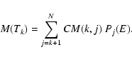
These considerations claim a statistical regularization process, which can be achieved by considering the histogram P(T) to be the statistical mean of 1000 histograms, all of them compatible with the observations according to Poisson statistics. For each one of the 1000 possible realizations for P_k(T), we have obtained the corresponding P_k(E) by means of the inversion of the integral equation. The non-physical histograms P_k(E), i.e., those with some negative bins, were rejected. From the physical solutions, we have obtained the mean histogram and the corresponding error bars, as shown in Fig. 11. The statistical regularization process also allows us to estimate errors due to the possible lack of statistics in the sample.

   
5.6 The probability distribution function of intrinsic ellipticities

In Fig. 11 we present the PDF of the bulge intrinsic ellipticities P(E). It was obtained by applying the procedure described in Sect. 5.5 using the PDF P(T) shown in Fig. 10. The T values for each galaxy were calculated by means of Eqs. (28) and (29) from the measured values of e, $\delta$ and $\theta$.

The PDF is characterized by a significant decrease of probability for E<0.07 (or equivalently B/A<0.93), suggesting that the shape of bulge ellipsoids in their equatorial plane is most probably elliptical rather than circular. Such a decrease is caused neither by the lack of statistics (because in the regularization method we took into account the Poisson noise) nor by the width of the bins (because we tried different bin widths).

We have calculated the average E value weighted with the PDF through

$$\langle E \rangle = \frac{\sum_{i}PDF(E_i) * E_i}{\sum_{i}PDF(E_i)},$$ (45)

obtaining a value of $\langle E \rangle = 0.16$ ( $\langle B/A \rangle = 0.85$). This is fully consistent with previous findings by Bertola et al. (1991) and Fathi & Peletier (2003), based on the analysis of smaller samples of bulges. For the sake of comparison, the value of $\langle B/A \rangle$ was derived from their data using Eq. (45). It is $\langle B/A \rangle = 0.85$ for the bulges studied by Bertola et al. (1991). They adopted a different approach to derive the PDF for intrinsic axial ratio of bulges from the misalignment of the major axes of bulges and disks and the apparent ellipticity of bulges. It is $\langle B/A \rangle = 0.79$for the early-type bulges of the sample studied by Fathi & Peletier (2003). They measured the bulge equatorial ellipticity by analyzing the deprojected ellipticity of the ellipses fitting the galaxy isophotes within the bulge radius.

	Figure 11: PDF of E. The probability is normalized over 10 bins, which are geometrically distributed to cover the interval (0,1). The width of the first bin is 0.03 and the width ratio of two consecutive bins is 1.25. The error bar of each Pk(E) bin corresponds to the Poisson statistics of 1000 realizations of Pk(T) after excluding non-physical cases.
Open with DEXTER

A further important result derived from P(E) is that there are not bulges with E>0.6 (B/A<0.5). This is also in good agreement with Bertola et al. (1991) and Fathi $\&$ Peletier (2003). They found a minimum axial ratio B/A=0.55 and B/A=0.45, respectively.

We also studied the possible differences in the shape of bulges depending on their observational characteristics (i.e., morphology, light concentration, and luminosity, see Fig. 12). First of all, we subdivided our bulges according to the morphological classification $-3 \leq HT <0$ and $0 \leq HT \leq 3$ of their host galaxies to look for differences between lenticular and early-type spiral galaxies. A second test was done by subdividing the sample bulge between those with a Sérsic index n<2 and those with $n \ge 2$ to investigate possible correlations of bulge shape with light concentration. Finally, we subdivided our bulge into faint ( $M_{\rm b} \ge -22$) and bright ( $M_{\rm b}<-22$) in order to search for differences of bulge shape with the J-band total luminosity. We did not find any significant difference between the studied subsamples. They are characterized by the same distribution of E, as confirmed at a high confidence level (>$99\%)$ by a Kolmogorov-Smirnov test.

Several authors discussed the problem of the intrinsic shape of elliptical galaxies by means of observations and/or numerical simulations. Ryden (1992), Lambas et al. (1992), and Bak & Statler (2000) agree that the observed distribution of ellipticities cannot be reproduced by any distribution of either prolate or oblate spheroidal systems. Any acceptable distribution of triaxial systems is dominated by nearly-oblate spheroidal rather than nearly-prolate spheroidal systems. The formation of triaxial elliptical galaxies via simulation of merging events in the framework of a hierarchical clustering assembly was studied by Barnes $\&$ Hernquist (1996), Naab $\&$ Burkert (2003) and Gonzalez-Garcia $\&$ Balcells (2005). On the other hand, in the monolithic scenario where the galaxy formation occurs at high redshift after a rapid collapse, we may expect that the final galaxy shape would be nearly spherical or axisymmetric, as recently found in numerical experiments by Merlin & Chiosi (2006). But there is no extensive testing of the predictions of numerical simulations against the derived distribution of bulge intrinsic ellipticities.

Figure 12: PDF of E for the different subsamples. (A) Lenticular galaxies ( $-3 \leq HT <0$). (B) Spiral galaxies ( $0 \leq HT \leq 3$). (C) Galaxies with $n\geq 2$. (D) Galaxies with n< 2. (E) Faint bulges ( $M_{\rm b}\geq -22$). (F) Bright bulges ( $M_{\rm b}<-22$). Bin widths and error bars as in Fig. 11. The mean intrinsic ellipticity and the number of galaxies of the subsample are given in each panel.

Open with DEXTER

5.7 The influence of nuclear bars on P(E)

The presence of nuclear bars in galaxy bulges has been known since the former work of de Vaucouleurs (1974). However, it is only in the last decade with the advent of high-resolution imaging that a large number of them have been detected allowing the study of their demography and properties (see Erwin 2004, and reference therein).

The sample galaxies were selected to not host large-scale bars, according to visual inspection and photometric decomposition of their J-band images (Sect. 2). These selection criteria did not account for the presence of nuclear bars. In fact, our sample has 23 galaxies in common with the samples studied by Mulchaey & Regan (1997), Jungwiert et al. (1997), Martini & Pogge (1999), Marquez et al. (1999) and Laine et al. (2002). They were interested in the demography of nuclear bars. A nuclear bar was found in 6 to 8 out of these 23 galaxies ($26\%$-$35\%$), according to the different authors' classifications.

Since nuclear bars are more elongated than their host bulges and have random orientations, they could affect the measurement of the structural parameters of bulges and consequently their P(E). To address this issue we carried out a series of simulations on a large set of artificial galaxies. They were obtained by adding a nuclear bar to the artificial image of a typical galaxy of the sample and analyzing the structural properties of the resulting image with GASP2D, as done in Sect. 3.1.

We adopted a Ferrers profile (Laurikainen et al. 2005) to describe the surface brightness of the nuclear bar component

   $$I_{\rm nb}(\xi,\eta) = \left\{\begin{array}{ll} I_{\rm0,nb}\l... ...}\\ 0 & {\rm if} \ r_{\rm nb} > a_{\rm nb} \end{array}\right.$$

where the coordinates $(\xi,\eta)$ are defined as in Sect. 3.1 and $a_{\rm nb}$, $I_{\rm0, nb}$, and $n_{\rm nb}$ are the bar length, its central surface brightness, and a shape parameter describing the curvature of the surface-brightness profile, respectively. Following Laurikainen et al. (2005) we chose $n_{\rm nb}=2$. Nuclear bar isophotes are ellipses centered on $(\xi_0,~\eta_0)$ with constant position angle PA$_{\rm nb}$ and constant ellipticity $\epsilon_{\rm nb} = 1 - q_{\rm nb}$. The radius $r_{\rm nb}$ is given by

 

$$r_{\rm nb} \left[(-(\xi-\xi_0) \sin{{\rm PA_{nb}}} + (\eta-\eta_0) \cos{{\rm PA_{nb}}})^2 \right.$$ =

$$- \left.((\xi-\xi_0) \cos{{\rm PA_{nb}}} + (\eta-\eta_0) \sin{{\rm PA_{nb}}})^2/q_{\rm nb}^2\right]^{1/2}.$$ (46)

We generated 1000 images of galaxies with a Sérsic bulge, an exponential disk, and a Ferrers nuclear bar. The structural parameters of the bulge and disk were selected to match those of a typical galaxy of the studied sample. It has J_T=9.6 mag, $r_{\rm e}=0.87$ kpc, n=2.32, h=2.47 kpc and B/T=0.37 according to the mean values of the structural parameters given in Table 3. Apparent ellipticity and position angle of the bulge and disk were randomly chosen in the ranges defined in Sect. 3.4. The structural parameters of the nuclear bar were randomly chosen in the ranges $0 < a_{\rm nb} < r_{\rm e}$ for the length, $0.2 < q_{\rm nb} < 0.7$ for the ellipticity, $0^\circ < {\rm PA_{nb}} < 180^\circ$for the position angle, and $0 < L_{\rm nb}/T < 0.02$ for the nuclear bar-to-total luminosity ratio.

The $a_{\rm nb}$ range was estimated from the 5 sample galaxies with a nuclear bar in common with Laine et al. (2002), which are characterized by $\langle a_{\rm nb}/r_{\rm e}\rangle=0.8$. Detailed studies about luminosities of nuclear bars are still missing. Nevertheless, the $L_{\rm nb}/T$ range was derived by considering that some nuclear bars are secondary bars, which reside in large-scale bars. According to Erwin & Sparke (2002), a typical secondary bar is about $12\%$ of the size of its primary bar. From Wozniak et al. (1995) we derived that the luminosity of the secondary bar is about $18\%$ of that of the primary one. Since a primary bar contributes about $15\%$ to the total luminosity of its galaxy (Laurikainen et al. 2005; Prieto et al. 2001), the typical $L_{\rm nb}/T$ ratio for a nuclear bar is about $2\%$.

All simulated galaxies were assumed at a distance of 30 Mpc. Pixel scale, CCD gain and RON, seeing, background level and photon noise of the artificial images were assumed as is Sect. 3.4. The two-dimensional parametric decomposition was applied by analyzing with GASP2D the images of the artificial galaxies as if they were real. We defined errors on the parameters as the difference between the input and output values. The mean errors on the fitted ellipticity and position angle of the bulge and disk and their standard deviation are given in Table 2. They correspond to systematic and typical errors.

Table 2: Errors on the ellipticity and position angles of the bulge and disk calculated for galaxies with nuclear bars by means of Monte Carlo simulations.

For each sample galaxy the values of e, $\delta$, and $\theta$ were derived in Sect. 5 from the ellipticity and position angle measured for the bulge and disk. We randomly generated a series of $q_{\rm b}$, $q_{\rm d}$, ${\rm PA_{\rm b}}$, and ${\rm PA_{\rm d}}$ by assuming they were normally distributed with the mean and standard deviation given in Table 2. We tested whether bulges are axisymmetric structures, which appear elongated and twisted with respect to the disk component due to the presence of a nuclear bar. To this aim, for each galaxy we selected 1000 realizations of $q_{\rm b}$, $q_{\rm d}$, ${\rm PA_{\rm b}}$, and ${\rm PA_{\rm d}}$ which gave smaller e (i.e., a rounder bulge) and smaller $\delta$ (i.e., a smaller misalignment between bulge and disk) with respect to the observed ones. This correction can be considered as an upper limit to the bulge axisymmetry. We obtained 1000 P(T)distributions and calculated P(E) from their mean.

Following this procedure, if we consider that all galaxies in our sample host a nuclear bar, we obtain a P(E) where the decrease of the probability for E<0.07 disappears (Fig. 13). This means that most of the bulges are circular in the equatorial plane. The average value of the ellipticity of $\langle E \rangle = 0.12$ ( $\langle B/A \rangle = 0.89$). However, if we consider a more realistic fraction of galaxies that host a nuclear bar (i.e., 30% as found by Laine et al. 2002 and Erwin & Sparke 2002), the resulting P(E) is consistent within errors with the P(E) derived in Sect. 5.6 (Fig. 13). The average value is $\langle E \rangle = 0.15$ ( $\langle B/A \rangle = 0.86$).

	Figure 13: PDF of E for the original sample (solid lines), for a sample with 30% of bulges with a nuclear bar (dotted line) and for a 100% fraction of galaxies hosting a nuclear bar (dashed line). Bin widths and error bars as in Fig. 11.
Open with DEXTER

   
6 Conclusions

The structural parameters of the bulge and disk of a magnitude-limited sample of 148 unbarred S0-Sb galaxies were investigated to constrain the dominant mechanism at the epoch of bulge assembly.

• We presented a new fitting algorithm (GASP2D) to perform two-dimensional photometric decomposition of galaxy images. The surface-brightness distribution of the galaxy was assumed to be the sum of the contribution of a Sérsic bulge and an exponential disk. The two components were characterized by elliptical and concentric isophotes with constant (but possibly different) ellipticity and position angles. GASP2D is optimized to deal with large image samples, and it adopts a robust Levenberg-Marquard fitting algorithm in order to obtain reliable estimates of the galaxy structural parameters.

• The bulge and disk parameters of the sample galaxies were derived from the J-band images, which were available in the Two Micron All Sky Survey.

• The bulges of the sample galaxies follow the same FP, FJ, and PP relationships found for elliptical galaxies. No statistically significant difference is observed when only bulges of lenticular and early-to-intermediate spiral galaxies were considered. This supports the idea that bulges and ellipticals formed in the same way.

• Tight correlations between the parameters of bulges and disks were found. In fact, the disk scale lengths increase with both the central velocity dispersion and bulge effective radius. Therefore, larger disks reside in galaxies with more massive and larger bulges. This was interpreted as an indication of the formation of bulges via secular evolution of their host disks.

• Our measurements of the exponential scale length of the bulge and disk, as well as of bulge shape parameter, were also fully consistent with numerical simulations of the effects of mergers on the mass distribution of the bulge and disk in galaxies formed in hierarchical clustering scenarios.

• These results indicate that the above relations are not enough to clearly distinguish between bulges formed by early dissipative collapse, merging or secular evolution. All these mechanisms could be tested against the intrinsic shape of bulges. Therefore, the PDF of the intrinsic equatorial ellipticity of the bulges was derived from the distribution of the observed ellipticities of bulges and their misalignments with disks.

• About $80\%$ of bulges in unbarred lenticular and early-to-intermediate spiral galaxies are not oblate but triaxial ellipsoids. Their mean axial ratio in the equatorial plane is $\langle B/A \rangle = 0.85$. This is consistent with previous findings by Bertola et al. (1991) and Fathi & Peletier (2003). There is no significant dependence of the PDF on the morphology, light concentration, and luminosity of bulges. The derived PDF is independent of the possible presence of nuclear bars.

Acknowledgements

J.M.A. acknowledges support from the Istituto Nazionale di Astrofisica (INAF). EMC receives support from grant PRIN2005/32 by Istituto Nazionale di Astrofisica (INAF) and from grant CPDA068415/06 by Padua University. J.A.L.A. acknowledges financial support by the Spanish Ministerio de Ciencia y Tecnologia grants AYA2004-08260-C03-01. ES acknowledges financial support by the Spanish Ministerio de Ciencia y Tecnologia grants AYA2004-08260-C03-01 and AYA2004-08243-C03-01, as well as by the European Assosciation for Research in Astronomy. JMA, EMC and ES acknowledge the Instituto de Astrofísica de Canarias for hospitality while this paper was in progress. We wish to thank P. B. Tissera for kindly provide us the data of their simulations and A. Pizzella and L. Morelli for useful discussions. We also thank the referee, R. F. Peletier, for insightful comments which helped to improve the original manuscript. This research has made use of the Lyon Meudon Extragalactic database (LEDA) and of the data products from the Two Micron All Sky Survey, which is a joint project of the University of Massachusetts and the Infrared Processing and Analysis Center/California Institute of Technology, funded by the National Aeronautics and Space Administration and the National Science Foundation.

References

• Aguerri, J. A. L., Balcells, M., & Peletier, R. F. 2001, A&A, 367, 428 [NASA ADS] [CrossRef] [EDP Sciences]
• Aguerri, J. A. L., Iglesias-Paramo, J., Vilchez, J. M., & Muñoz-Tuñón, C. 2004, AJ, 127, 1344 [NASA ADS] [CrossRef]
• Aguerri, J. A. L., Elias-Rosa, N., Corsini, E. M., & Muñoz-Tuñón, C. 2005a, A&A, 434, 109 [NASA ADS] [CrossRef] [EDP Sciences]
• Aguerri, J. A. L., Iglesias-Páramo, J., Vílchez, J. M., Muñoz-Tuñón, C., & Sánchez-Janssen, R. 2005b, AJ, 130, 475 [NASA ADS] [CrossRef]
• Amorín, R. O., Muñoz-Tuñón, C., Aguerri, J. A. L., Cairós, L. M., & Caon, N. 2007, A&A, 467, 541 [NASA ADS] [CrossRef] [EDP Sciences]
• Andredakis, Y. C., & Sanders, R. H. 1994, MNRAS, 267, 283 [NASA ADS]
• Andredakis, Y. C., Peletier, R. F., & Balcells, M. 1995, MNRAS, 275, 874 [NASA ADS]
• Athanassoula, E. 2005, MNRAS, 358, 1477 [NASA ADS] [CrossRef]
• Bak, J., & Statler, T. S. 2000, AJ, 120, 110 [NASA ADS] [CrossRef]
• Balcells, M., Graham, A. W., & Peletier, R. F. 2007, ApJ, 665, 1104 [NASA ADS] [CrossRef]
• Baugh, C. M., Cole, S., & Frenk, C. S. 1996, MNRAS, 283, 1361 [NASA ADS]
• Barnes, J. E., & Hernquist, L. 1996, ApJ, 471, 115 [NASA ADS] [CrossRef]
• Bender, R., Burstein, D., & Faber, S. M. 1992, ApJ, 399, 462 [NASA ADS] [CrossRef] (In the text)
• Bender, R., Burstein, D., & Faber, S. M. 1993, ApJ, 411, 153 [NASA ADS] [CrossRef] (In the text)
• Berman, S. 2001, A&A, 371, 476 [NASA ADS] [CrossRef] [EDP Sciences]
• Bernardi, M., Sheth, R. K., Annis, J., et al. 2003, AJ, 125, 1866 [NASA ADS] [CrossRef] (In the text)
• Bertin, E., & Arnouts, S. 1996, A&AS, 117, 393 [NASA ADS] [CrossRef] [EDP Sciences] (In the text)
• Bertola, F., Zeilinger, W. W., & Rubin, V. C. 1989, ApJ, 345, L29 [NASA ADS] [CrossRef]
• Bertola, F., Vietri, M., & Zeilinger, W. W. 1991, ApJ, 374, L13 [NASA ADS] [CrossRef] (In the text)
• Binggeli, B., & Jerjen, H. 1998, A&A, 333, 17 [NASA ADS]
• Burstein, D., Bender, R., Faber, S., & Nolthenius, R. 1997, AJ, 114, 1365 [NASA ADS] [CrossRef]
• Byun, Y. I., & Freeman, K. C. 1995, ApJ, 448, 563 [NASA ADS] [CrossRef] (In the text)
• Caon, N., Capaccioli, M., & D'Onofrio, M. 1993, MNRAS, 265, 1013 [NASA ADS] (In the text)
• Caon, N., Cairós, L. M., Aguerri, J. A. L., & Muñoz-Tuñón, C. 2005, ApJS, 157, 218 [NASA ADS] [CrossRef]
• Cappellari, M., Bacon, R., Bureau, M., et al. 2006, MNRAS, 366, 1126 [NASA ADS]
• Carollo, C. M. 1999, ApJ, 523, 566 [NASA ADS] [CrossRef] (In the text)
• Carollo, C. M., Stiavelli, M., & Mack, J. 1998, AJ, 116, 68 [NASA ADS] [CrossRef]
• Coccato, L., Corsini, E. M., Pizzella, A., et al. 2004, A&A, 416, 507 [NASA ADS] [CrossRef] [EDP Sciences] (In the text)
• Coccato, L., Corsini, E. M., Pizzella, A., & Bertola, F. 2005, A&A, 440, 107 [NASA ADS] [CrossRef] [EDP Sciences] (In the text)
• Cole, S., Lacey, C. G., Baugh, C. M., & Frenk, C. S. 2000, MNRAS, 319, 168 [NASA ADS] [CrossRef]
• Combes, F., Debbasch, F., Friedli, D., & Pfenniger, D. 1990, A&A, 233, 82 [NASA ADS] (In the text)
• Corsini, E. M., Debattista, V. P., & Aguerri, J. A. L. 2003a, ApJ, 599, L29 [NASA ADS] [CrossRef] (In the text)
• Corsini, E. M., Pizzella, A., Coccato, L., & Bertola, F. 2003b, A&A, 408, 873 [NASA ADS] [CrossRef] [EDP Sciences] (In the text)
• Courteau, S., de Jong, R. S., & Broeils, A. H. 1996, ApJ, 457, L73 [NASA ADS] [CrossRef] (In the text)
• Davies, R. L., & Illingworth, G. 1983, ApJ, 266, 516 [NASA ADS] [CrossRef]
• Debattista, V. P., Carollo, C. M., Mayer, L., & Moore, B. 2004, ApJ, 604, L93 [NASA ADS] [CrossRef]
• de Jong, R. S. 1996, A&AS, 118, 557 [NASA ADS] [CrossRef] [EDP Sciences]
• de Souza, R. E., Gadotti, D., & dos Anjos, S. 2004, ApJS, 153, 411 [NASA ADS] [CrossRef]
• de Vaucouleurs, G. 1974, The Formation and Dynamics of Galaxies, 58, 335 [NASA ADS]
• de Vaucouleurs, G., de Vaucouleurs, A., Corwin, H. G., Jr., et al. 1991, S&T, 82, 621 [NASA ADS]
• Djorgovski, S., & Davis, M. 1987, ApJ, 313, 59 [NASA ADS] [CrossRef]
• Dressler, A., Lynden-Bell, D., Burstein, D., et al. 1987, ApJ, 313, 42 [NASA ADS] [CrossRef]
• Eggen, O. J., Lynden-Bell, D., & Sandage, A. R. 1962, ApJ, 136, 748 [NASA ADS] [CrossRef]
• Eliche-Moral, M. C., Balcells, M., Aguerri, J. A. L., & González-García, A. C. 2006, A&A, 457, 91 [NASA ADS] [CrossRef] [EDP Sciences]
• Elmegreen, B. G., Elmegreen, D. M., & Hirst, A. C. 2004, ApJ, 612, 191 [NASA ADS] [CrossRef]
• Erwin, P. 2004, A&A, 415, 941 [NASA ADS] [CrossRef] [EDP Sciences] (In the text)
• Erwin, P., & Sparke, L. S. 2002, AJ, 124, 65 [NASA ADS] [CrossRef]
• Eskridge, P. B., Frogel, J. A., Pogge, R. W., et al. 2000, AJ, 119, 536 [NASA ADS] [CrossRef]
• Faber, S. M., & Jackson, R. E. 1976, ApJ, 204, 668 [NASA ADS] [CrossRef] (In the text)
• Falcón-Barroso, J., Peletier, R. F., & Balcells, M. 2002, MNRAS, 335, 741 [NASA ADS] [CrossRef]
• Fathi, K., & Peletier, R. F. 2003, A&A, 407, 61 [NASA ADS] [CrossRef] [EDP Sciences] (In the text)
• Freeman, K. C. 1970, ApJ, 160, 811 [NASA ADS] [CrossRef] (In the text)
• Gerhard, O. E., & Vietri, M. 1986, MNRAS, 223, 377 [NASA ADS]
• Gerhard, O. E., Vietri, M., & Kent, S. M. 1989, ApJ, 345, L33 [NASA ADS] [CrossRef]
• Gilmore, G., & Wyse, R. F. G. 1998, AJ, 116, 748 [NASA ADS] [CrossRef]
• González-García, A. C., & Balcells, M. 2005, MNRAS, 357, 753 [NASA ADS] [CrossRef]
• Graham, A. W., & Guzmán, R. 2003, AJ, 125, 2936 [NASA ADS] [CrossRef] (In the text)
• Greusard, D., Friedli, D., Wozniak, H., Martinet, L., & Martin, P. 2000, A&AS, 145, 425 [NASA ADS] [CrossRef] [EDP Sciences]
• Hunt, L. K., Pierini, D., & Giovanardi, C. 2004, A&A, 414, 905 [NASA ADS] [CrossRef] [EDP Sciences]
• Jarrett, T. H., Chester, T., Cutri, R., et al. 2000, AJ, 119, 2498 [NASA ADS] [CrossRef] (In the text)
• Jogee, S., Barazza, F. D., Rix, H.-W., et al. 2004, ApJ, 615, L105 [NASA ADS] [CrossRef]
• Jorgensen, I., Franx, M., & Kjaergaard, P. 1995, MNRAS, 276, 1341 [NASA ADS]
• Jungwiert, B., Combes, F., & Axon, D. J. 1997, A&AS, 125, 479 [NASA ADS] [CrossRef] [EDP Sciences]
• Kauffmann, G. 1996, MNRAS, 281, 487 [NASA ADS]
• Kent, S. M. 1985, ApJS, 59, 115 [NASA ADS] [CrossRef] (In the text)
• Khosroshahi, H. G., Wadadekar, Y., & Kembhavi, A. 2000, ApJ, 533, 162 [NASA ADS] [CrossRef]
• Kormendy, J. 1977, ApJ, 217, 406 [NASA ADS] [CrossRef]
• Kormendy, J. 1993, Galactic Bulges, 153, 209 [NASA ADS]
• Kormendy, J., & Illingworth, G. 1982, ApJ, 256, 460 [NASA ADS] [CrossRef]
• Kormendy, J., & Kennicutt, R. C., Jr. 2004, ARA&A, 42, 603 [NASA ADS] [CrossRef]
• Kormendy, J., Bender, R., & Bower, G. 2002, The Dynamics, Structure & History of Galaxies: A Workshop in Honour of Professor Ken Freeman, 273, 29
• Laine, S., Shlosman, I., Knapen, J. H., & Peletier, R. F. 2002, ApJ, 567, 97 [NASA ADS] [CrossRef]
• Lambas, D. G., Maddox, S. J., & Loveday, J. 1992, MNRAS, 258, 404 [NASA ADS]
• Laurikainen, E., Salo, H., & Buta, R. 2005, MNRAS, 362, 1319 [NASA ADS] [CrossRef] (In the text)
• Lindblad, B. 1956, Stockholms Observatoriums Annaler, 2,
• MacArthur, L. A., Courteau, S., & Holtzman, J. A. 2003, ApJ, 582, 689 [NASA ADS] [CrossRef]
• Márquez, I., Durret, F., Delgado, R. M. G., et al. 1999, A&AS, 140, 1 [NASA ADS] [CrossRef] [EDP Sciences]
• Martinez-Valpuesta, I., Shlosman, I., & Heller, C. 2006, ApJ, 637, 214 [NASA ADS] [CrossRef]
• Martini, P., & Pogge, R. W. 1999, AJ, 118, 2646 [NASA ADS] [CrossRef]
• Matkovic, A., & Guzmán, R. 2005, MNRAS, 362, 289 [NASA ADS] [CrossRef] (In the text)
• Menéndez-Delmestre, K., Sheth, K., Schinnerer, E., Jarrett, T. H., & Scoville, N. Z. 2007, ApJ, 657, 790 [NASA ADS] [CrossRef]
• Merlin, E., & Chiosi, C. 2006, A&A, 457, 437 [NASA ADS] [CrossRef] [EDP Sciences]
• Möllenhoff, C., & Heidt, J. 2001, A&A, 368, 16 [NASA ADS] [CrossRef] [EDP Sciences]
• Möllenhoff, C. 2004, A&A, 415, 63 [NASA ADS] [CrossRef] [EDP Sciences]
• Moré, J. J., Garbow, B. S., & Hillstrom, K. E. 1980, User guide for MINPACK-1, Argonne National Laboratory Report ANL-80-74
• Mulchaey, J. S., & Regan, M. W. 1997, ApJ, 482, L135 [NASA ADS] [CrossRef]
• Naab, T., & Burkert, A. 2003, ApJ, 597, 893 [NASA ADS] [CrossRef]
• Naab, T., & Trujillo, I. 2006, MNRAS, 369, 625 [NASA ADS] [CrossRef]
• Paturel, G., Petit, C., Prugniel, P., et al. 2003, A&A, 412, 45 [NASA ADS] [CrossRef] [EDP Sciences] (In the text)
• Peng, C. Y., Ho, L. C., Impey, C. D., & Rix, H. 2002, AJ, 124, 266 [NASA ADS] [CrossRef] (In the text)
• Pfenniger, D., & Norman, C. 1990, ApJ, 363, 391 [NASA ADS] [CrossRef] (In the text)
• Pignatelli, E., Fasano, G., & Cassata, P. 2006, A&A,446, 373
• Press, W. H., Teukolsky, S. A., Vetterling, W. T., & Flannery, B. P. 1996, Numerical Recipes in Fortran 77: The Art of Scientific Computing (Cambridge: Cambridge University Press) (In the text)
• Prieto, M., Aguerri, J. A. L., Varela, A. M., & Muñoz-Tuñón, C. 2001, A&A, 367, 405 [NASA ADS] [CrossRef] [EDP Sciences] (In the text)
• Raha, N., Sellwood, J. A., James, R. A., & Kahn, F. D. 1991, Nature, 352, 411 [NASA ADS] [CrossRef]
• Regan, M. W., & Mulchaey, J. S. 1999, AJ, 117, 2676 [NASA ADS] [CrossRef]
• Ryden, B. 1992, ApJ, 396, 445 [NASA ADS] [CrossRef]
• Sandage, A. 1990, JRASC, 84, 70 [NASA ADS]
• Scannapieco, C., & Tissera, P. B. 2003, MNRAS, 338, 880 [NASA ADS] [CrossRef]
• Searle, L., & Zinn, R. 1978, ApJ, 225, 357 [NASA ADS] [CrossRef]
• Sersic, J. L. 1968, Cordoba, Argentina: Observatorio Astronomico, 1968, (In the text)
• Simard, L. 1998, in Astronomical Data Analysis Software Systems VII, ed. R. Albrecht, R. N. Hook, & H. A. Bushouse (San Francisco: ASP), ASP Conf. Ser., 145, 108
• Simonneau, E., Varela, A. M., & Muñoz-Tuñón, C. 1998, Nuovo Cimento B Serie, 113, 927 [NASA ADS] (In the text)
• Skrutskie, M. F., Cutri, R. M., Stiening, R., et al. 2006, AJ, 131, 1163 [NASA ADS] [CrossRef] (In the text)
• Thakar, A. R., & Ryden, B. S. 1998, BAAS, 30, 1408 [NASA ADS] (In the text)
• Tissera, P. B., Smith Castelli, A. V., & Scannapieco, C. 2006, A&A, 455, 135 [NASA ADS] [CrossRef] [EDP Sciences]
• Tonry, J. L., Dressler, A., Blakeslee, J. P., et al. 2001, ApJ, 546, 681 [NASA ADS] [CrossRef]
• Trujillo, I., Aguerri, J. A. L., Cepa, J., & Gutiérrez, C. M. 2001a, MNRAS, 328, 977 [NASA ADS] [CrossRef]
• Trujillo, I., Aguerri, J. A. L., Cepa, J., & Gutiérrez, C. M. 2001b, MNRAS, 321, 269 [NASA ADS] [CrossRef]
• Trujillo, I., Aguerri, J. A. L., Gutiérrez, C. M., & Cepa, J. 2001c, AJ, 122, 38 [NASA ADS] [CrossRef] (In the text)
• Wozniak, H., Friedli, D., Martinet, L., Martin, P., & Bratschi, P. 1995, A&AS, 111, 115 [NASA ADS]
• Wyse, R. F. G., Gilmore, G., & Franx, M. 1997, ARA&A, 35, 637 [NASA ADS] [CrossRef]
• Zaritsky, D., & Lo, K. Y. 1986, ApJ, 303, 66 [NASA ADS] [CrossRef]

 

  
Online Material

Table 3: Main properties and structural bulge and disk parameters of the galaxies in the sample.