A&A 466, 1-9 (2007)
DOI: 10.1051/0004-6361:20065714
V. N. Zirakashvili1,2
1 - Pushkov Institute of Terrestrial Magnetism, Ionosphere and Radiowave
Propagation, 142190 Troitsk, Moscow Region, Russia
2 -
Max-Planck-Institut für Kernphysik, 69029 Heidelberg, Postfach 103980, Germany
Received 29 May 2006 / Accepted 2 November 2006
Abstract
Using a so-called hemispherical model we
derive a general transport equation for cosmic ray and thermal particles scattered
in pitch angle by magnetic inhomogeneities in a moving collisionless plasma.
The weak scattering through 90 degrees results in
isotropic particle distributions in each hemisphere. The consideration is not limited
by small anisotropies and by the condition that
particle velocities are higher than characteristic flow velocity differences.
For high velocities and small
anisotropies the standard
cosmic ray transport equation is recovered. We apply the equations derived for
investigation of injection and acceleration of particles by collisionless shocks.
Key words: acceleration of particles - cosmic rays
Progress in cosmic ray astrophysics has been made with the introduction of the transport equation for cosmic rays (Krymsky 1964; Parker 1965; Dolginov & Toptygin 1966; Gleeson & Axford 1969). It was successfully applied to many astrophysical problems: cosmic ray modulation in the solar wind, acceleration of particles at shock fronts, cosmic ray propagation in the Galaxy etc. This equation implies that in the strong scattering approximation the particle distribution is almost isotropic, which in particular implies that velocities of particles are higher than the characteristic flow velocity differences in the plasma. However, in several circumstances these conditions are violated and more general kinetic equations should be used which also deal with the evolution of the pitch angle distribution. Since the solution of such equations is not a simple task, we would like find a description that comes close to that implied by the standard transport equation.
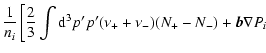
Energetic particles are scattered in pitch angle relative to the mean magnetic field direction by random magnetic inhomogeneities. It is well known that in the case of particle transport along the mean magnetic field a so-called problem of scattering through the pitch-angle of 90 degrees exist. According to quasilinear theory the resonant scattering of particles is weak at small pitch-angle cosines (Jokipii 1966). The main reason for this phenomenon is the small energy density of short waves propagating along the magnetic field and scattering the particles with pitch angles close to 90 degrees. These waves may be easily damped by thermal ions. Even without such a damping, the scattering in the vicinity of 90 degrees is depressed in the case of a power-law spectrum of waves that is proportional to k-2 or steeper. Here k is the wavenumber. This problem can be avoided if one takes into account the scattering by oblique waves or nonlinear interactions, for example magnetic mirroring (see e.g. Völk 1973, 1975; Achterberg 1981). One can expect that the scattering efficiency is small near the pitch angle of 90 degrees.
Observations of suprathermal pick-up particles in the solar wind suggest that this is the case (Fisk et al. 1997). If the scattering through 90 degrees is weak, the particle distribution is almost isotropic in each hemisphere of the velocity directions parallel or antiparallel to the mean field. So, in this case the angular dependence of particle distribution is reduced to the two number densities of forward and backward moving particles. The corresponding equations were derived by Isenberg (1997) for the case of pick-up ions in the solar wind.
We use this approach and derive general transport equations for arbitrary nonrelativistic flow velocities. We use the particle distributions in the frame moving with the medium. This permits us to consider the case of arbitrary particle velocities. Since the number density of particles in both hemispheres may substantially differ, large anisotropies can also be taken into account. The equations derived have a broad range of applicability: propagation of solar energetic particles and pick-up ions in the solar wind, injection into diffusive shock acceleration and other processes.
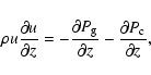
As an example of the application of the equations derived, we consider the problem of diffusive shock acceleration. Since our equations describe propagation of thermal as well as energetic particles in the vicinity of the collisionless shock front, they can be used for the determination of the shock velocity profile and the spectra of thermal and nonthermal particles without any assumptions regarding the injection efficiency. One only has to prescribe the scattering law. In this sense the approach is similar to the one used by Ellison & Eichler (1984). They applied a Monte-Carlo technique for the solution of the kinetic equation.
The basis of such an approach is the idea that the interaction of upstream and downstream plasmas may result in instabilities similar to firehose instability (Parker 1961; Quest 1988). The magnetic inhomogeneities produced by such instabilities may play the role of scattering centers and provide the shock dissipation and heating. These ideas are also the basis of the so-called hybrid simulations of collisionless shocks (Leroy & Winske 1983; Quest 1986). The ions move in self-consistent electromagnetic fields and the electrons are considered as a charged neutralizing fluid in these simulations.
The equations are derived in the next two sections. Application to the case of collisionless shock is considered in Sects. 4 and 5. Section 6 contains a discussion of results obtained and conclusions.
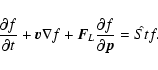
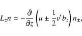
We start with the kinetic equation for the momentum distribution
![]() of charged particles
of charged particles
 |
(1) |
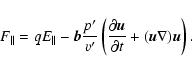
![\begin{displaymath}%
{\vec E}=E_\parallel {\vec b}-\frac 1c[{\vec u}\times {\vec B}],
\end{displaymath}](/articles/aa/full/2007/16/aa5714-06/img14.gif) |
(2) |
It is convenient to perform a change of variable ![]() to
to ![]() that formally
coincides with the nonrelativistic Lorence transform
that formally
coincides with the nonrelativistic Lorence transform
 |
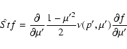
(3) |
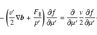
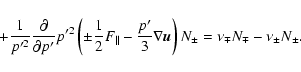
![\begin{eqnarray*}\frac {\partial f}{\partial t}+(v'\mu '{\vec b}+{\vec u})\nabla f=\hat {St} f\\ [1mm]
\end{eqnarray*}](/articles/aa/full/2007/16/aa5714-06/img22.gif)
![\begin{eqnarray*}+\frac {\partial f}{\partial p'}\left[
\frac {3\mu '^2-1}{2}p'
...
...1-\mu '^2}{2}p'\nabla {\vec u}-\mu 'F_\parallel
\right]\\ [2mm]
\end{eqnarray*}](/articles/aa/full/2007/16/aa5714-06/img23.gif)
![\begin{displaymath}%
+\frac {\partial f}{\partial \mu '}(1-\mu '^2)\left[
\frac ...
...rac {\mu '}{2}\nabla {\vec u}-\frac {F_\parallel }{p'}
\right]
\end{displaymath}](/articles/aa/full/2007/16/aa5714-06/img24.gif) |
(4) |
 |
(5) |
 |
(6) |
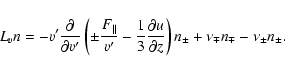
Let us assume that the scattering frequency is large for pitch angle cosines
![]() .
The momentum distribution f is then isotropic in these regions of the angle space.
We introduce distributions of particles in the backward and forward hemispheres
.
The momentum distribution f is then isotropic in these regions of the angle space.
We introduce distributions of particles in the backward and forward hemispheres ![]() :
:
![]() for
for
![]() and
and
![]() for
for
![]() .
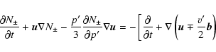
Integration of Eq. (4) from -1 to
.
Integration of Eq. (4) from -1 to ![]() and from
and from ![]() to 1 gives the equations for these distributions:
to 1 gives the equations for these distributions:
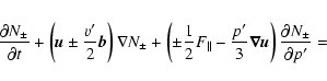
 |
(7) |
 |
(8) |
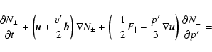
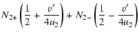
| (9) |
![\begin{displaymath}%
\nu _\pm (p')=\pm \frac {\frac {F_\parallel }{p'}+\frac {v'...
...frac {2F_\parallel }{v'p'}+\nabla {\vec b}\right) \right] -1},
\end{displaymath}](/articles/aa/full/2007/16/aa5714-06/img47.gif) |
(10) |
 |
(11) |
We neglected the derivatives in time and space in Eq. (8). This assumption
is valid if the characteristic time ![]() and the characteristic scale l of the
problem considered are large enough:
and the characteristic scale l of the
problem considered are large enough:
![]() .
Since
.
Since
![]() ,
our derivation is valid even if the scale l is comparable with the
mean free path
,
our derivation is valid even if the scale l is comparable with the
mean free path ![]() .
Equation (9) is exact in the mathematical limit
.
Equation (9) is exact in the mathematical limit
![]() ,
,
![]() .
.
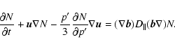
Equations (9) can be rewritten in the conservative form:
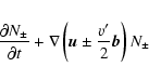  |
(12) |
It is clear that the system of Eq. (12) is hyperbolic. It
can be reduced to uncoupled equations for N+ and N-:
![\begin{eqnarray*}\left. +
\frac {1}{p'^2}\frac {\partial }{\partial p'}p'^2
\lef...
... {p'}{3}{\bf\nabla} {\vec u}\right)
\right] \frac {1}{2\nu _\mp}
\end{eqnarray*}](/articles/aa/full/2007/16/aa5714-06/img58.gif)
![\begin{displaymath}%
\times\left[ \frac {\partial N_\pm }{\partial t}+
\left( {\...
...vec u}\right)
\frac {\partial N_\pm }{\partial p'}\right]\cdot
\end{displaymath}](/articles/aa/full/2007/16/aa5714-06/img59.gif) |
(13) |
 |
(14) |
Another interesting case is when the energy changes and transport by
the medium are negligible. Then Eq. (13) is reduced to the so-called
telegraph equation (cf. Fisk & Axford 1969):
![\begin{displaymath}%
\frac {\partial N_\pm }{\partial t}=
-\left[ \frac {\partia...
...}{\partial t}
\pm \frac {v'}{2}({\vec b}\nabla )N_\pm \right].
\end{displaymath}](/articles/aa/full/2007/16/aa5714-06/img63.gif) |
(15) |
The equations derived in the previous section contain prescribed values for the
flow velocities ![]() ,
the
parallel force
,
the
parallel force
![]() and the magnetic field
and the magnetic field ![]() .
Such a description is a good
approximation for the investigation of propagation of test particles. However, in many
interesting cases these quantities should be determined self-consistently, involving the
distributions N+ and N-.
.
Such a description is a good
approximation for the investigation of propagation of test particles. However, in many
interesting cases these quantities should be determined self-consistently, involving the
distributions N+ and N-.
We treat electrons as a massless fluid. In this case the Euler equation for electrons
is reduced to an expression for the electric field:
![\begin{displaymath}%
{\vec E +\delta {\vec E}}= -\frac {\nabla P_{\rm e}}{qn_{\r...
...c 1c[{\vec u}_{\rm e}\times ({\vec B} +{\bf\delta} {\vec B})],
\end{displaymath}](/articles/aa/full/2007/16/aa5714-06/img64.gif) |
(16) |
![\begin{displaymath}%
[{\bf\nabla} \times ({\vec B}+{\bf\delta} {\vec B})]=\frac ...
... q}{c}
\int {\rm d}^3p({\vec v}-{\vec u}_{\rm e})(f+\delta f),
\end{displaymath}](/articles/aa/full/2007/16/aa5714-06/img70.gif) |
(17) |
![\begin{eqnarray*}{\vec E}= -\frac 1c[{\vec u}\times {\vec B}]-
\frac {1}{qn_{\rm...
...vec B}\times [\nabla \times {\vec B}]]+
\nabla P_{\rm e}
\right.
\end{eqnarray*}](/articles/aa/full/2007/16/aa5714-06/img72.gif)
 |
(18) |
We multiply Eq. (1) containing the electric field (18) by
![]() and integrate
over momentum space. This gives the Euler equation of motion:
and integrate
over momentum space. This gives the Euler equation of motion:
![\begin{displaymath}%
\rho \left( \frac {\partial {\vec u}}{\partial t}+
({\vec u...
...\times [{\bf\nabla} \times {\vec B}]]-
\nabla (P_{\rm e}+P_i).
\end{displaymath}](/articles/aa/full/2007/16/aa5714-06/img78.gif) |
(19) |
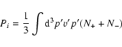 |
(20) |
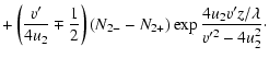
Since the Eq. (1) with the electric field (18) conserves momentum, the same is true for Eq. (9). Let us multiply them by p', integrate over
![]() and subtract the first from the second. This gives after some algebra
and subtract the first from the second. This gives after some algebra
| |
= |  |
|
![$\displaystyle \left.+ {\vec b}\left( \frac {\partial {\vec u}}{\partial t}+
({\...
...t {\rm d}^3p''
\left( \frac {p''}{v''}-\frac {p'}{v'}\right) (N_++N_-)
\right].$](/articles/aa/full/2007/16/aa5714-06/img84.gif) |
(21) |
We shall assume an adiabatic evolution of the electron pressure
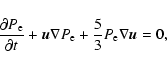 |
(22) |
![\begin{displaymath}%
\frac {\partial \vec B}{\partial t}=
[\nabla \times [{\vec u}\times {\vec B}]].
\end{displaymath}](/articles/aa/full/2007/16/aa5714-06/img86.gif) |
(23) |
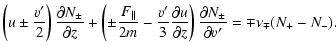
Let us consider the acceleration at the parallel one-dimensional shock. We can write the steady-state version of Eq. (9) for nonrelativistic particles in the shock frame as
 |
(24) |
The characteristics of this system of equations for the case
![]() are given by
are given by
 |
(25) |
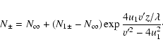
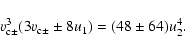
There is an another possibility for the initial acceleration. If the initial speed of the backward moving particle upstream is high enough, say 0.7u1, it can reach the line u=v'/2 directly and return upstream with an energy gain. However, the initial speed is rather high. The number of such particles is small for high Mach number shocks.
The characteristics of Eq. (24) depend on
![]() .
The characteristics for
the case
.
The characteristics for
the case
![]() are shown in Fig. 2. This case is close to the real situation
because the two first terms in Eq. (21) almost cancel each other (see also the numeric modeling below). In other words, the electric force
are shown in Fig. 2. This case is close to the real situation
because the two first terms in Eq. (21) almost cancel each other (see also the numeric modeling below). In other words, the electric force
![]() almost compensate the inertia
force
almost compensate the inertia
force
![]() in the second term on the left-hand side of Eq. (24).
This is not a simple coincidence. The electric force is the consequence of the momentum
transfer and is approximately
in the second term on the left-hand side of Eq. (24).
This is not a simple coincidence. The electric force is the consequence of the momentum
transfer and is approximately
![]() that is
exactly
that is
exactly
![]() .
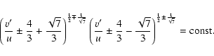
The characteristics are determined by expressions
.
The characteristics are determined by expressions
 |
(26) |
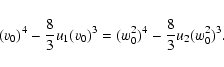
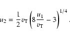
We find the analytical solution of Eq. (24) for the case when the
velocity profile is discontinuous: u(z)=u1, z<0 and u(z)=u2, z>0. In the
regions of constant velocity u the system (24) can be rewritten as (to be
compared with Gombosi et al. 1993)
 |
(27) | ||
 |
(28) |
 |
(29) |
| (30) |
| |
= |  |
|
 |
(31) |
| (32) |
We find the relation between the upstream and downstream
distributions ![]() and
and ![]() .
It depends on the solution of
Eq. (24) in the transition region. We consider the case
.
It depends on the solution of
Eq. (24) in the transition region. We consider the case
![]() .
Then the distributions upstream and downstream
are related by characteristics (26):
.
Then the distributions upstream and downstream
are related by characteristics (26):
 |
(33) |
Let us consider the case
![]() .
Since the change of
velocity in the transition region is governed by the characteristics (26), the
solution is the following sum of
.
Since the change of
velocity in the transition region is governed by the characteristics (26), the
solution is the following sum of ![]() -functions:
-functions:
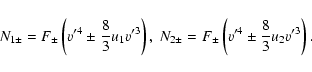
![\begin{displaymath}%
N_{1\pm }=A_{0}\delta (v'-v_{0})/(v_{0})^2 +
\sum ^2_{j=1}\...
...nfty _{i=1}A^j_{i\pm }\delta (v'-v^j_{i})/(v^j_{i})^2,\\ [3mm]
\end{displaymath}](/articles/aa/full/2007/16/aa5714-06/img114.gif) |
(34) |
 |
(35) |
If the upstream sequences
![]() are known for v'>2u1the downstream ones can be found from characteristics (26). Using the properties of
are known for v'>2u1the downstream ones can be found from characteristics (26). Using the properties of
![]() -functions we find that they are given by
-functions we find that they are given by
 |
(36) |
 |
(37) |
 |
(38) |
 |
(39) |
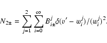
Let us introduce the critical velocities ![]() .
They are the
solutions of equations:
.
They are the
solutions of equations:
 |
(40) |
1)
v0<vc-. Forward and backward moving particles reach the downstream region with
velocities smaller than 2u2 and are further advected. The injection in acceleration
does not occur. The downstream coefficients
![]() are given by
are given by
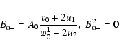
 |
(41) |
 |
(42) |
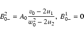
2)
![]() .
The most important case for injection. The forward moving particle
reaches the downstream region with a velocity less than 2u2 and again is not injected into
acceleration. The coefficients
.
The most important case for injection. The forward moving particle
reaches the downstream region with a velocity less than 2u2 and again is not injected into
acceleration. The coefficients
![]() and
and
![]() are the same as in the previous case.
are the same as in the previous case.
The backward moving particle goes
along characteristics and returns upstream (see Fig. 2). Using properties of ![]() -functions in Eq. (33) and conditions (30) we found
-functions in Eq. (33) and conditions (30) we found
 |
(43) |
 |
(44) |
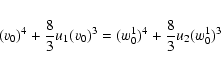
3)
![]() .
Forward and backward moving particles reach the downstream region with
velocities greater than 2u2 and are injected into acceleration. The coefficients
.
Forward and backward moving particles reach the downstream region with
velocities greater than 2u2 and are injected into acceleration. The coefficients
![]() and
and
![]() are the same as in the previous case. The coefficients
are the same as in the previous case. The coefficients
![]() are given by
are given by
 |
(45) |
 |
(46) |
4) v0>2u1. The coefficients
![]() and
and
![]() at i>0can be found consecutively using Eqs. (36)-(39).
at i>0can be found consecutively using Eqs. (36)-(39).
Using Eqs. (36) and (38) one can relate
Aji+1+ and Aji+:
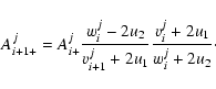 |
(47) |
It is easy to show that for large wji and vji the change of
velocity
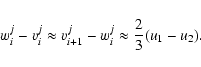 |
(48) |
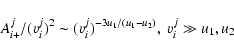 |
(49) |
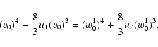
The solution for u1/u2=4 and
v0=0.25u1 is shown in Fig. 3. The
critical velocities are
![]() and
and
![]() in this case.
The far upstream distribution is shown by the dashed line on the left. The forward moving
particles of this distribution reach the downstream region with slightly higher velocity
(solid line on the left). The backward moving particles are directly accelerated along
the characteristic and return upstream with a velocity close to 8u1/3 (first dashed line
on the right). Particles are accelerated further, moving between downstream and upstream
regions of the shock (the other lines on the right). The similar
in this case.
The far upstream distribution is shown by the dashed line on the left. The forward moving
particles of this distribution reach the downstream region with slightly higher velocity
(solid line on the left). The backward moving particles are directly accelerated along
the characteristic and return upstream with a velocity close to 8u1/3 (first dashed line
on the right). Particles are accelerated further, moving between downstream and upstream
regions of the shock (the other lines on the right). The similar ![]() -function
spectrum was obtained by Bogdan & Webb (1987) for cosmic ray acceleration in
the so-called two-streaming
approximation of Fisk & Axford (1969).
-function
spectrum was obtained by Bogdan & Webb (1987) for cosmic ray acceleration in
the so-called two-streaming
approximation of Fisk & Axford (1969).
The spectrum will be smoother if one takes into account the scattering of particles in the transition region.
We use the system of Eqs. (12), (19), (22), (23) for the modeling of
steady-state one-dimensional nonrelativistic shocks.
We neglect the dynamical effects of the magnetic
field, which means that the magnetic field produces only kinematic effects that are
essential for oblique shocks. The upstream plasma state is then determined only by the
sonic shock Mach number M and by the ratio of electron and ion temperatures
![]() .
.
A so-called Alfvén heating is not included in our model. It is well known
that the energetic particles upstream of the shock can effectively generate
Alfvén waves due to streaming instability (Wentzel 1969;
Bell 1978). The damping of these waves results in the heating of the shock
precursor (Völk & McKenzie 1982; McKenzie & Völk 1982).
This heating is essential,
since it decreases the effective Mach number and compression ratio of the shock.
As shown in the Appendix, this effect can be formally included using the
relation between sonic and Alfvén Mach numbers of the shock:
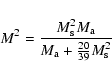 |
(50) |
The details of the numeric method are given in the Appendix. The plasma flow with unity velocity and unity density enters the simulation box from its left boundary. The pressure at the right boundary was adjusted according to the motion of the shock in order to reach the steady state. We used the free escape boundary condition for the particle distribution at the left boundary.
We prescribe the dependence of the free path of particles on the velocity v' and
space coordinate z. We used the free path ![]() that is independent on z. This is not
a strong limitation. Indeed, in the rather general case of separable dependence of
that is independent on z. This is not
a strong limitation. Indeed, in the rather general case of separable dependence of ![]() on v' and z, the results obtained depend only on the integral
on v' and z, the results obtained depend only on the integral
![]() .
Thus
our results can be used also for this more general case.
.
Thus
our results can be used also for this more general case.
The energy dependence of the mean free path ![]() is determined by the spectrum of magnetic
inhomogeneities and by the mechanism of scattering in the vicinity of a pitch angle of 90 degrees. Since the low frequency waves propagating along the magnetic field are subject to nonlinear
wave steepening,
one can expect that the magnetic spectra are close to k-2 and the corresponding free path
does not depend on energy. Such spectra (or slightly flatter ones) were indeed observed
in the hybrid plasma simulations of parallel collisionless shocks
(Giacalone et al. 1993; Giacalone 2004) and in the vicinity of
the Earth bow shock in the solar wind. In the results presented here we used the energy independent
free path.
is determined by the spectrum of magnetic
inhomogeneities and by the mechanism of scattering in the vicinity of a pitch angle of 90 degrees. Since the low frequency waves propagating along the magnetic field are subject to nonlinear
wave steepening,
one can expect that the magnetic spectra are close to k-2 and the corresponding free path
does not depend on energy. Such spectra (or slightly flatter ones) were indeed observed
in the hybrid plasma simulations of parallel collisionless shocks
(Giacalone et al. 1993; Giacalone 2004) and in the vicinity of
the Earth bow shock in the solar wind. In the results presented here we used the energy independent
free path.
We limit ourselves to the case of cold electrons
![]() ,
as
the dissipation of the Alfvén waves in the precursor may result in the preferable heating
of ions. The solar corona is an example of this.
,
as
the dissipation of the Alfvén waves in the precursor may result in the preferable heating
of ions. The solar corona is an example of this.
We start with the case of parallel shocks with Mach numbers 3.87 and 7.75. According to Eq. (50) the corresponding Alfvén Mach numbers are 7.5 and 30 that can be applied to the interplanetary and supernova shocks respectively. The downstream particle distributions are shown in the top panels of Figs. 4 and 5. The velocity and gas pressure profiles are shown in the bottom panels.
The simulated shocks demonstrate clear sub-shocks with a width of about one half
of the free path ![]() and a smooth precursor produced by the particles in the
high energy tail that is seen in the top panels of Figs. 4 and 5. It was found that the main part of the downstream distribution in Figs. 4 and 5 is the adiabatically compressed far upstream
distribution which was taken to be Maxwellian. The total electric potential corresponding
to the electric force
and a smooth precursor produced by the particles in the
high energy tail that is seen in the top panels of Figs. 4 and 5. It was found that the main part of the downstream distribution in Figs. 4 and 5 is the adiabatically compressed far upstream
distribution which was taken to be Maxwellian. The total electric potential corresponding
to the electric force
![]() is about 0.2-0.3 mu12 according to Figs. 4 and 5.
is about 0.2-0.3 mu12 according to Figs. 4 and 5.
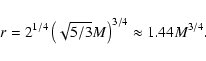
The total compression ratio of the shock can be found from the following simple estimate.
In the precursor region the thermal particles are heated adiabatically. When their
velocities become comparable to the plasma velocity, the backward moving particles
are accelerated more efficiently (see Fig. 2) and injected for further
acceleration. The compression ratio should be large enough for this to be the case.
For estimation we assume that distribution of upstream particles is
proportional to
![]() ,
where
,
where
![]() is the thermal
velocity of the plasma. The maximum shock downstream velocity u2 that is necessary for
injection of such particles according to Fig. 2 and characteristics (26) is
is the thermal
velocity of the plasma. The maximum shock downstream velocity u2 that is necessary for
injection of such particles according to Fig. 2 and characteristics (26) is
 |
(51) |
 |
(52) |
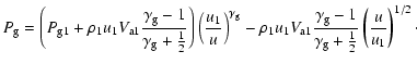
This compression ratio is close to the maximum
possible compression ratio of the idealized system that includes the infinitely
thin gas sub-shock and the viscous precursor produced by energetic particles. Using
the Ranke-Hugoniot conditions at the thermal sub-shock one can obtain for this case:
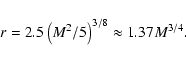 |
(53) |
The comparison of our results and results obtained for this simplified
description are shown in Fig. 6.
The Eq. (14) was solved in the upstream region together with the Euler equations.
The top panel shows the comparison of
downstream spectra obtained in these approaches. The velocity profiles are
compared in the bottom panel. We find a very good agreement of these two methods.
We estimate the injection efficiency at injection velocity
![]() to be about 0.024. Here
to be about 0.024. Here
![]() is the sub-shock velocity.
This number is in reasonable agreement with results of hybrid simulations
(cf. Giacalone et al. 1993; Ellison et al. 1993)
and the Earth bow shock observations (cf. Ellison et al. 1990).
is the sub-shock velocity.
This number is in reasonable agreement with results of hybrid simulations
(cf. Giacalone et al. 1993; Ellison et al. 1993)
and the Earth bow shock observations (cf. Ellison et al. 1990).
We have also performed modeling of a quasi-parallel shock. The results obtained for
a Mach number of 7.75 and an angle between the shock normal and magnetic field of
![]() are shown in Fig. 7.
are shown in Fig. 7.
For such oblique shocks the dip appears between the main part of the thermal distribution
and the high-energy tail (see the top panel). The injection efficiency is the same as in the
previous case.
![]() is the maximal value of
is the maximal value of ![]() that allows us to model steady state shocks with M=7.75. Even this value is rather large, because it corresponds to the normal angle 40
that allows us to model steady state shocks with M=7.75. Even this value is rather large, because it corresponds to the normal angle 40![]() upstream of the thermal subshock.
For larger
upstream of the thermal subshock.
For larger ![]() this dip becomes more pronounced and the thermal subshock
width drops to a grid step. In some cases some instability in the downstream region
was observed. It is possible to model the larger values of
this dip becomes more pronounced and the thermal subshock
width drops to a grid step. In some cases some instability in the downstream region
was observed. It is possible to model the larger values of ![]() for the smaller Mach numbers
(e.g.
for the smaller Mach numbers
(e.g.
![]() for M=3.87).
Thus our approach can be used only for quasiparallel shocks with the normal
angle less than 40
for M=3.87).
Thus our approach can be used only for quasiparallel shocks with the normal
angle less than 40![]() just upstream of the thermal subshock.
just upstream of the thermal subshock.
If the magnetic field is oblique enough, it prevents particles from returning from downstream along magnetic lines and the heating of particles is impossible. Since it is necessary to have the energetic particles downstream for the existence of a shock, we expect that the transition region will be squeezed to widths of the order of the ion gyroradius. Heating then may take place in a different regime, where the drift motion of particles perpendicular to magnetic field is essential. The injection efficiency also may be very different.
Many astrophysical problems deal with collisionless plasma. Different low frequency instabilities may produce magnetic inhomogeneities that can scatter particles and play the role of thermal collisions. When unstable waves propagate preferably along the mean magnetic field, the resonant scattering of particles is weak in the vicinity of 90 degrees pitch angle. In this case it is possible that particle distributions are almost isotropic in both hemispheres.
Following the approach of Isenberg (1997) we derive the general transport Eq. (12) (or equivalent Eq. (9)) which takes into account the motion of the medium and energy changes of particles. Our consideration is not limited by high particle velocities and by small anisotropies of particle distribution.
In the case of high particle velocities and small anisotropies the equation derived can be reduced to the standard cosmic ray transport equation. In the case of negligible energy changes and advective transport the equation may be transformed to the so-called telegraph equation.
The equations derived can be solved together with magnetohydrodynamic equations (see Sect. 3). We used the fluid approximation for the electron transport. This is justified if electrons are effectively scattered by magnetic inhomogeneities. If this is not the case, one can use Eqs. (12) for electron transport. In this way electron injection at collisionless shocks can be investigated.
The transport Eqs. (12) with Eqs. (19), (22) and (23) can be used for the solution of different astrophysical problems when the self-consistent determination of the flow velocity, magnetic field etc. is necessary.
We apply the equation derived to investigate particle acceleration and injections at astrophysical shocks. For the prescribed velocity profile we have found the exact analytical solution (see Sect. 4).
We also have performed the modeling of collisionless shocks and found a formula for the shock compression ratio (see Eq. (52)). This ratio is very close to the maximal possible value in the framework of the simplified approach used for cosmic ray modified shocks. The corresponding thermal sub-shock ratio is 2.5.
We found that this feature is universal and does not depend on the maximum
energy of the accelerated particles. This was checked in our simulations up to
the maximum momentum
![]() which was limited by the step of
our uniform spatial grid. This property will not change for
higher maximum energies corresponding to the supernova environment. On the other
hand we found that the injection efficiency
which was limited by the step of
our uniform spatial grid. This property will not change for
higher maximum energies corresponding to the supernova environment. On the other
hand we found that the injection efficiency ![]() is not universal.
For
is not universal.
For
![]() it is about 0.024 for an injection
velocity equal to two sub-shock velocities. It slowly decreased as the maximum
energy increases and is about 0.003 for young supernova remnants.
This is because at small maximum energies the thermal ions "feel'' a larger
compression ratio than the thermal subshock compression ratio since the subshock
and precursor width are not strongly different.
it is about 0.024 for an injection
velocity equal to two sub-shock velocities. It slowly decreased as the maximum
energy increases and is about 0.003 for young supernova remnants.
This is because at small maximum energies the thermal ions "feel'' a larger
compression ratio than the thermal subshock compression ratio since the subshock
and precursor width are not strongly different.
We found that the equations derived can be used to investigate injection and
acceleration in quasiparallel shocks with the subshock normal angle
![]() .
The
dissipation at more oblique shocks is described by a different mechanism which
takes into account the motion of particles in the direction perpendicular to the magnetic
field. The injection efficiency at such shocks is unknown, but it is possible
that it is rather low. We confirm the previous findings that quasiparallel
shocks are very efficient accelerators with high injection efficiency
(see e.g. Ellison & Eichler 1984; Giacalone et al. 1993;
Malkov & Drury 2001) which does not
depend on the angle
.
The
dissipation at more oblique shocks is described by a different mechanism which
takes into account the motion of particles in the direction perpendicular to the magnetic
field. The injection efficiency at such shocks is unknown, but it is possible
that it is rather low. We confirm the previous findings that quasiparallel
shocks are very efficient accelerators with high injection efficiency
(see e.g. Ellison & Eichler 1984; Giacalone et al. 1993;
Malkov & Drury 2001) which does not
depend on the angle ![]() (Giacalone et al. 1997).
(Giacalone et al. 1997).
Acknowledgements
The author is grateful to Heinz Völk for fruitful discussions of the collisionless shock physics. The author also thanks the anonymous referee for important comments.
The heating of the cosmic ray precursor is described by the
following equations (Völk & McKenzie 1982; McKenzie & Völk 1982):
 |
(A.1) |
 |
(A.2) |
 |
(A.3) |
The gradient of the cosmic ray pressure can be found from Eq. (A.2) and substituted
into Eq. (A.3). For high Mach number shocks the solution can be written as
 |
(A.4) |
For high Mach number shocks the Alfvén heating is essential only at the
very beginning of the precursor. In the rest, the gas is heated adiabatically
and the last term in Eq. (A.4) can be neglected. The gas pressure
![]() and Alfvén velocity
and Alfvén velocity
![]() can be expressed in terms of Alfvén and
sonic Mach numbers
can be expressed in terms of Alfvén and
sonic Mach numbers ![]() and
and ![]() respectively. As a result, we obtain the
sonic Mach number M of the shock without Alfvén heating, which is equivalent to
the shock with the Alfvén heating:
respectively. As a result, we obtain the
sonic Mach number M of the shock without Alfvén heating, which is equivalent to
the shock with the Alfvén heating:
 |
(A.5) |
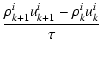
We used the implicit finite difference scheme for the solution of the one-dimensional
version of Eq. (12):
 |
(B.1) |
 |
(B.2) |
 |
(B.3) |
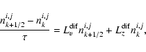 |
(B.4) |
 |
(B.5) |
| |
= | 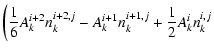 |
|
 |
(B.6) |
| |
= | 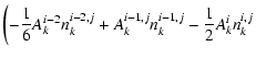 |
|
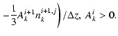 |
(B.7) |
The numeric scheme (B.4), (B.5) with these operators has a third order accuracy on z and v' and first order accuracy on t.
The parallel force
![]() was recalculated at each time step according to
Eq. (21). The medium velocity uki at each time step was calculated
according to the finite difference version of the Euler Eq. (19):
was recalculated at each time step according to
Eq. (21). The medium velocity uki at each time step was calculated
according to the finite difference version of the Euler Eq. (19):
 |
= |  |
|
 |
(B.8) |
 |
(B.9) |
We use the hyperbolic tangent for the initial velocity profile. The initial
particle distribution was Maxwellian with a temperature and density dependence
corresponding to the momentum and mass conservation. At times of about 60-100 in dimensionless
units the system reaches the steady state. We use 200 grid points in the z-direction,
100 grid points for the logarithmic v' grid and the time step between 0.005 and 0.1 for
different runs. We obtained the total momentum, energy and mass conservation with
several percent accuracy.
![\begin{figure}
\par\includegraphics[angle=270,width=8.2cm,clip]{5714fig1.ps}\end{figure}](/articles/aa/full/2007/16/aa5714-06/img90.gif)
![\begin{figure}
\par\includegraphics[angle=270,width=8.2cm,clip]{5714fig2.ps}\end{figure}](/articles/aa/full/2007/16/aa5714-06/img96.gif)
![\begin{figure}
\par\includegraphics[angle=270,width=8.15cm,clip]{5714fig3.ps}\end{figure}](/articles/aa/full/2007/16/aa5714-06/img146.gif)
![\begin{figure}
\par\includegraphics[width=8.4cm,clip]{5714fig4.ps}\end{figure}](/articles/aa/full/2007/16/aa5714-06/img156.gif)
![\begin{figure}
\par\includegraphics[width=8.4cm,clip]{5714fig5.ps}\end{figure}](/articles/aa/full/2007/16/aa5714-06/img157.gif)
![\begin{figure}
\par\includegraphics[width=8.4cm,clip]{5714fig6.ps}\end{figure}](/articles/aa/full/2007/16/aa5714-06/img164.gif)
![\begin{figure}
\par\includegraphics[width=8.4cm,clip]{5714fig7.ps}\end{figure}](/articles/aa/full/2007/16/aa5714-06/img168.gif)