A&A 461, 775-781 (2007)
DOI: 10.1051/0004-6361:20065788
A. Kellerer1 - A. Tokovinin2
1 - European Southern Observatory,
Karl-Schwarzschild-Strasse 2, 85748
Garching bei München, Germany
2 -
Cerro Tololo Inter-American Observatory, Casilla 603, La Serena,
Chile
Received 9 June 2006 / Accepted 15 September 2006
Abstract
Aims. Current and future ground-based interferometers require knowledge of the atmospheric time constant t0, but this parameter has diverse definitions. Moreover, adequate techniques for monitoring t0 still have to be implemented.
Methods. We derive a new formula for the structure function of the fringe phase (piston) in a long-baseline interferometer, and review available techniques for measuring the atmospheric time constant and the shortcomings.
Results. It is shown that the standard adaptive-optics atmospheric time constant is sufficient for quantifying the piston coherence time, with only minor modifications. The residual error of a fast fringe tracker and the loss of fringe visibility in a finite exposure time are calculated in terms of the same parameter. A new method based on the fast variations of defocus is proposed. The formula for relating the defocus speed to the time constant is derived. Simulations of a 35-cm telescope demonstrate the feasibility of this new technique for site testing.
Key words: atmospheric effects - instrumentation: interferometers - site testing
Astronomical sites for classical observations are characterized in terms of atmospheric image quality (seeing). For high-angular resolution techniques such as adaptive optics (AO) and interferometry, we need to know additional parameters. The atmospheric coherence time is one of these. Here we refine the definition of the interferometric coherence time, review available techniques, and propose a new method for its measurements.
The AO time constant, ![]() , is a well-defined parameter
related to the vertical distribution of turbulence and wind speed
(Roddier 1981). To correct wave fronts in real time, a
sufficient number of photons from the guide star is needed within each coherence
area during time
, is a well-defined parameter
related to the vertical distribution of turbulence and wind speed
(Roddier 1981). To correct wave fronts in real time, a
sufficient number of photons from the guide star is needed within each coherence
area during time ![]() .
This severely restricts the
choice of natural guide stars and tends to impose the complex use of
laser guide stars (Hardy 1998). It is shown below that new,
simple methods of
.
This severely restricts the
choice of natural guide stars and tends to impose the complex use of
laser guide stars (Hardy 1998). It is shown below that new,
simple methods of ![]() monitoring are still needed.
monitoring are still needed.
Modern ground-based stellar interferometers attain extreme resolution,
but their sensitivity is limited by the atmosphere. Even at the best
observing sites, such as Paranal in Chile, fast fringe tracking is not
fully operative yet, and one therefore tends to employ exposure
times that are short enough to "freeze" the atmospheric turbulence.
The price is a substantial loss in limiting magnitude. It is hence
important to measure the time constant, t0, of the piston
- i. e. the mean phase over the telescope aperture - at existing and
future sites.
However, the exact definition of t0 is not clear, any
more than are methods to measure it. Do we need an interferometer to
evaluate t0? Is t0 different from ![]() ? Does it depend on the
aperture size and baseline?
We review various definitions of the interferometric time constant
based on the piston structure function (SF), on the error of a fringe tracker,
and on the loss of fringe contrast during a finite exposure time.
It is shown that the piston time constant is
proportional to the AO coherence time
? Does it depend on the
aperture size and baseline?
We review various definitions of the interferometric time constant
based on the piston structure function (SF), on the error of a fringe tracker,
and on the loss of fringe contrast during a finite exposure time.
It is shown that the piston time constant is
proportional to the AO coherence time ![]() ,
both depending on the
same combination of atmospheric parameters.
,
both depending on the
same combination of atmospheric parameters.
During site exploration campaigns, one
would like to predict the performance of large base-line
interferometers, and it is desirable to do this with single-dish and,
preferably, small telescopes. The existing techniques
for ![]() measurement are listed and a new method for site
testing proposed.
measurement are listed and a new method for site
testing proposed.
First, we introduce the relevant atmospheric parameters and the AO
time constant ![]() .
For convenience, we outline the essential
formulae, but for the general background, we refer the reader
to Roddier (1981).
.
For convenience, we outline the essential
formulae, but for the general background, we refer the reader
to Roddier (1981).
The spatial and temporal fluctuations of atmospheric phase distortion
![]() are usually described by the SF
are usually described by the SF
The atmosphere consists of many layers. The contribution of a layer i of thickness dhat altitude h
to the turbulence intensity is specified in terms of
![]() ,
equivalently expressed through the Fried parameter
,
equivalently expressed through the Fried parameter
![]() ,
,
![]() being the wavenumber.
The spatial SF in the inertial range (between
inner and outer scales) is
being the wavenumber.
The spatial SF in the inertial range (between
inner and outer scales) is
It is assumed that each layer moves as a whole with the velocity
vector
![]() (Taylor hypothesis).
The temporal SF of the
piston fluctuations
(Taylor hypothesis).
The temporal SF of the
piston fluctuations
![]() in one small aperture due to
a single layer is then equal to the spatial SF at shift V t,
in one small aperture due to
a single layer is then equal to the spatial SF at shift V t,
In an interferometer with a large baseline
(![]() ,
where L0: turbulence outer scale)
the phase patterns over
the apertures are uncorrelated on short time scales. Thus, for a
small time interval (t < B/V), the SF of the phase difference
,
where L0: turbulence outer scale)
the phase patterns over
the apertures are uncorrelated on short time scales. Thus, for a
small time interval (t < B/V), the SF of the phase difference
![]() (do not confuse with the phase
(do not confuse with the phase ![]() )
in an
interferometer with two small apertures will simply be two times
larger,
)
in an
interferometer with two small apertures will simply be two times
larger,
![]() (Conan et al. 1995).
As a result the
differential piston variance reaches 1 rad2 for a time delay
(Conan et al. 1995).
As a result the
differential piston variance reaches 1 rad2 for a time delay
![]() .
Note that in the case of smaller baselines and large outer scales
- when the assumption
.
Note that in the case of smaller baselines and large outer scales
- when the assumption ![]() becomes invalid -
becomes invalid -
![]() and the resulting coherence time, accordingly, lies between
and the resulting coherence time, accordingly, lies between
![]() and
and ![]() .
Yet,
.
Yet, ![]() applies to the characterization of large baseline interferometers at low-turbulence sites.
applies to the characterization of large baseline interferometers at low-turbulence sites.
When an interferometer with larger circular apertures of diameter d is
considered, phase fluctuations are averaged inside each aperture. As
shown later, for time increments smaller than d/V, the piston
structure function is quadratic in t and is essentially determined
by the average wave-front tilt over the aperture. The variance of the
gradient tilt ![]() (in radians) in one direction is
(Roddier 1981, Conan et al. 1995, Sasiela 1994)
(in radians) in one direction is
(Roddier 1981, Conan et al. 1995, Sasiela 1994)
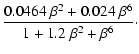
Note that for small time intervals there is a weak dependence of the SF on the aperture diameter. Also, the wind velocity averaging is slightly modified. However, the expressions for t1 and t0produce similar numerical results as long as d/r0 is not too large. Thus, the system-independent definition of the AO time constant (4) also gives a good description of the temporal variations of the piston.
For time delays of approximately B/V and larger, the pistons on two
apertures are no longer independent. However,
estimates of the time interval over which the Taylor hypothesis is valid
range from ![]() 40 ms (Schoeck & Spillar 1998)
to several seconds (Colavita et al. 1987).
Hence, at time intervals of 1 s or more, the Taylor hypothesis is insecure.
Moreover, the finite
turbulence outer scale reduces the amplitude of slow piston variations
substantially. Here we concentrate only on rapid piston variations
where our approximations are valid.
40 ms (Schoeck & Spillar 1998)
to several seconds (Colavita et al. 1987).
Hence, at time intervals of 1 s or more, the Taylor hypothesis is insecure.
Moreover, the finite
turbulence outer scale reduces the amplitude of slow piston variations
substantially. Here we concentrate only on rapid piston variations
where our approximations are valid.
![\begin{figure}
\par\includegraphics[width=8cm]{5788fig1.ps}\end{figure}](/articles/aa/full/2007/02/aa5788-06/img47.gif) |
Figure 1:
Theoretical temporal power spectrum of the fringe position at
0.5 |
| Open with DEXTER | |
The temporal power spectrum of the atmospheric fringe position has been
derived by Conan et al. (1995). Their result is reproduced
in Appendix A with minor changes. The temporal piston power spectrum
(A.4) produced by a single turbulent layer is represented in
Fig. 1 for a specific set of parameters.
Because of the
infinite outer scale L0, this example is not realistic for
frequencies below ![]() 1 Hz.
Moreover, as discussed in Sect. 2.2, Taylor's frozen flow hypothesis
becomes invalid at low frequencies.
Due to the infinite L0, the asymptotic behavior of the spectrum, and
in particular the cut-off frequencies, do not depend on the
wind direction (Conan et al. 1995),
whereas, in the real case of a finite outer scale,
the cut-off frequencies are affected by wind direction,
as described by Avila et al. (1997).
Conan et al. (1995) point out
that changing turbulence intensity and wind speed shift the spectrum
vertically and horizontally, respectively, without changing the shape
of the curve on the log-log plot.
In observations with a small baseline (
1 Hz.
Moreover, as discussed in Sect. 2.2, Taylor's frozen flow hypothesis
becomes invalid at low frequencies.
Due to the infinite L0, the asymptotic behavior of the spectrum, and
in particular the cut-off frequencies, do not depend on the
wind direction (Conan et al. 1995),
whereas, in the real case of a finite outer scale,
the cut-off frequencies are affected by wind direction,
as described by Avila et al. (1997).
Conan et al. (1995) point out
that changing turbulence intensity and wind speed shift the spectrum
vertically and horizontally, respectively, without changing the shape
of the curve on the log-log plot.
In observations with a small baseline (![]() 12 m), the proportionality
to
12 m), the proportionality
to
![]() at low frequencies and to
at low frequencies and to
![]() at medium
frequencies has actually been measured, e.g. by Colavita et al. (1987).
at medium
frequencies has actually been measured, e.g. by Colavita et al. (1987).
![\begin{figure}
\par\includegraphics[width=8cm]{5788fig2.ps}
\end{figure}](/articles/aa/full/2007/02/aa5788-06/img49.gif) |
Figure 2:
Relation between average wind velocities
|
| Open with DEXTER | |
![\begin{figure}
\par\includegraphics[width=7.5cm]{5788fig3.ps}\end{figure}](/articles/aa/full/2007/02/aa5788-06/img51.gif) |
Figure 3:
Structure function of the fringe position for an interferometer with mirror diameters d = 0.1 m,
r0 = 11 cm, V = 10 m/s. The vertical line corresponds to t = d/V.
For t < d/V, the SF is quadratic in t (dotted line), cf. Eq. (7).
For longer time scales,
|
| Open with DEXTER | |
Based on the piston power spectrum, we derive in Appendix A the
new expression of the piston SF valid for time increments
![]() :
:
![\begin{figure}
\par\includegraphics[width=8cm]{5788fig4.ps}\end{figure}](/articles/aa/full/2007/02/aa5788-06/img58.gif) |
Figure 4:
Variance of corrected fringe position as a function of the
bandwidth frequency of the correction system. The parameters of the
simulation are identical to those of Fig. 1.
At frequencies higher than
|
| Open with DEXTER | |
A fringe tracker measures the position of the central fringe and
computes a correction. The actual compensation equals the integrated
corrections applied after each iteration. Our analysis is similar to
the classical work by Greenwood & Fried (1976).
For a more detailed model that takes the effect
of the finite exposure and response times of the phasing device into account,
see the work by Conan et al. (2000b).
The error transfer function of a first-order phase-tracking loop equals
| (9) |
Table 1: Definitions of atmospheric time constants.
Table 1 assembles different definitions of the atmospheric
coherence time. We have demonstrated that the time constant t0 of
the piston SF is proportional to the AO time constant ![]() .
For
small time increments, a slightly modified parameter t1 should be used.
.
For
small time increments, a slightly modified parameter t1 should be used.
A different, but essentially equivalent, definition of the piston
coherence time
![]() has been given by Tango & Twiss (1980) and reproduced by
Colavita et al. (1987). It is the integration time during
which the piston variance equals 1 rad2. When fringes are integrated
over a time T0, the mean decrease in squared visibility equals 1/e.
Here we use the more convenient definition
has been given by Tango & Twiss (1980) and reproduced by
Colavita et al. (1987). It is the integration time during
which the piston variance equals 1 rad2. When fringes are integrated
over a time T0, the mean decrease in squared visibility equals 1/e.
Here we use the more convenient definition
![]() based
on the temporal SF and warn against confusion with Tango's
T0. The definition of T0 is valid only for T > d/V, while
shorter integration times are of practical interest (see below).
based
on the temporal SF and warn against confusion with Tango's
T0. The definition of T0 is valid only for T > d/V, while
shorter integration times are of practical interest (see below).
The performance of the fringe-tracker in a long-baseline
interferometer can be characterized by the atmospheric time constant
t1 or, equivalently, by the average wind speed
![]() .
The AO time constant
.
The AO time constant ![]() (or
(or
![]() )
is also a good
estimator of the piston coherence time, especially for small apertures
)
is also a good
estimator of the piston coherence time, especially for small apertures
![]() .
.
In order to reach a good magnitude limit, all modern interferometers
have large apertures d>r0. The atmospheric variance over the
aperture is
![]() rad2 and has to be corrected by
some means (tip-tilt guiding, full AO correction, spatial filtering of
the PSF) even at short integration times. The temporal piston
variance will also be >1 rad2 on time scales of approximately
rad2 and has to be corrected by
some means (tip-tilt guiding, full AO correction, spatial filtering of
the PSF) even at short integration times. The temporal piston
variance will also be >1 rad2 on time scales of approximately
![]() and longer.
Hence exposure times shorter than
and longer.
Hence exposure times shorter than
![]() or fast fringe
trackers are required in order to maintain high fringe
contrast. In this regime, the relevant time constant
that determines the visibility loss is t1, rather than
or fast fringe
trackers are required in order to maintain high fringe
contrast. In this regime, the relevant time constant
that determines the visibility loss is t1, rather than ![]() and T0.
and T0.
All definitions of atmospheric time constants contain a combination of
r0 and
![]() .
As turbulence becomes stronger, the time
constant decreases, although the wind speed may remain unchanged.
Being less correlated, the parameters
.
As turbulence becomes stronger, the time
constant decreases, although the wind speed may remain unchanged.
Being less correlated, the parameters
![]() are thus
more suitable for characterizing atmospheric turbulence than the
parameters
are thus
more suitable for characterizing atmospheric turbulence than the
parameters
![]() .
Astronomical sites with "slow'' or
"fast'' seeing should be ranked in terms of
.
Astronomical sites with "slow'' or
"fast'' seeing should be ranked in terms of
![]() rather
than
rather
than ![]() .
A fair correlation between
.
A fair correlation between
![]() and the wind
speed at 200 mB altitude has been noted by Sarazin & Tokovinin
(2002).
and the wind
speed at 200 mB altitude has been noted by Sarazin & Tokovinin
(2002).
Table 2:
Methods of ![]() measurement.
measurement.
Table 2 lists methods available for measuring the atmospheric
coherence time ![]() or related parameters. The 3rd
column gives an indicative diameter of the telescope aperture required for each method.
Short comments on each technique are given below.
or related parameters. The 3rd
column gives an indicative diameter of the telescope aperture required for each method.
Short comments on each technique are given below.
SCIDAR (SCIntillation Detection And Ranging) has provided good results
on ![]() .
It is not suitable for
monitoring because manual data processing is still needed to extract
V(h), despite efforts to automate the process. Balloons provide
only single-shot profiles of low individual statistical
significance. The AO systems and interferometers give reliable results,
but are not suitable for testing new sites or for long-term monitoring.
.
It is not suitable for
monitoring because manual data processing is still needed to extract
V(h), despite efforts to automate the process. Balloons provide
only single-shot profiles of low individual statistical
significance. The AO systems and interferometers give reliable results,
but are not suitable for testing new sites or for long-term monitoring.
The methods listed in the next four rows of Table 2 all
require small telescopes and can thus be used for site-testing.
However, all these techniques have some intrinsic problems.
SSS (Single Star SCIDAR) essentially extends the SCIDAR technique to small telescopes:
profiles of Cn2 (h) and V(h) are obtained with lower height
resolution than with the SCIDAR, and are then used to derive the coherence time.
The GSM (Generalized Seeing Monitor) can only measure velocities of
prominent layers after careful data processing.
A coherence time, ![]() -
which, however, does not have a similar dependence on the turbulence
profile than
-
which, however, does not have a similar dependence on the turbulence
profile than ![]() and t1 -
is deduced from the angle of arrival fluctuations.
MASS (Multi-Aperture Scintillation Sensor) is a recent, but already well-proven,
turbulence monitor. One of its observables related to scintillation
in a 2 cm aperture approximates
and t1 -
is deduced from the angle of arrival fluctuations.
MASS (Multi-Aperture Scintillation Sensor) is a recent, but already well-proven,
turbulence monitor. One of its observables related to scintillation
in a 2 cm aperture approximates
![]() (Tokovinin
2002), but this averaging does not include low layers and thus
gives a biased estimate of
(Tokovinin
2002), but this averaging does not include low layers and thus
gives a biased estimate of ![]() .
An even less secure evaluation
of
.
An even less secure evaluation
of ![]() can be obtained from DIMM (Differential Image Motion Monitor)
by combining the measured r0with meteorological data on the wind speed (Sarazin & Tokovinin
2002).
can be obtained from DIMM (Differential Image Motion Monitor)
by combining the measured r0with meteorological data on the wind speed (Sarazin & Tokovinin
2002).
We conclude from this brief survey that a correct yet simple technique
for measuring ![]() with a small-aperture telescope is still
lacking. Such a method is proposed in the next section.
with a small-aperture telescope is still
lacking. Such a method is proposed in the next section.
| |
Figure 5:
Five consecutive ring images distorted by turbulence and
detector noise. Each image is
|
| Open with DEXTER | |
![\begin{figure}
\mbox{
\includegraphics[width=8.5cm]{5788fig6.ps} \includegraphics[width=8.5cm]{5788fig7.ps} }\end{figure}](/articles/aa/full/2007/02/aa5788-06/img89.gif) |
Figure 6: Temporal structure functions of simulated measurements of the ring radius for wind speeds 10 m/s ( left) and 20 m/s ( right) and r0 = 0.1 m seeing (time constants t1 of 3.36 and 1.68 ms, respectively). |
| Open with DEXTER | |
To measure the interferometric or AO time constant, we need an
observable related to
![]() or
or
![]() .
The
atmosphere consists of many layers with different wind speeds and
directions, so a true Cn2-weighted estimator (5) is
required. Its response should be independent of the wind direction.
.
The
atmosphere consists of many layers with different wind speeds and
directions, so a true Cn2-weighted estimator (5) is
required. Its response should be independent of the wind direction.
Wavefront distortions are commonly decomposed into Zernike modes (Noll 1976). The first mode, piston, cannot be sensed with a single telescope and the two subsequent modes, tip and tilt, tend to be corrupted by telescope vibrations. Of the remaining modes, the next three - defocus and two astigmatisms - have the highest variance and are the best candidates for measuring atmospheric parameters.
The total turbulence integral (or r0) is typically measured by the
DIMM (Sarazin & Roddier 1990).
Lopez (1992) tried to derive ![]() from the speed of the DIMM
signal, but this method did not prove to be practical. Because of its
intrinsic asymmetry, DIMM does not provide an estimator of
from the speed of the DIMM
signal, but this method did not prove to be practical. Because of its
intrinsic asymmetry, DIMM does not provide an estimator of
![]() that is independent of the wind direction. On the
other hand, the fourth Zernike mode (defocus) is rotationally symmetric.
that is independent of the wind direction. On the
other hand, the fourth Zernike mode (defocus) is rotationally symmetric.
We show in Appendix B that the variance of defocus velocity provides an
estimator of the time constant t1. The variance of the defocus
itself gives a measure of r0. Thus, we can measure both r0 and
![]() .
The method is based on series of fast-defocus
measurements, and we call it FADE (FAst DEfocus).
The details of the future FADE instrument still need to be worked out
and will be a subject of the forthcoming paper.
Here we present
numerical simulations to show the feasibility of this approach. We
simulated a telescope of d = 0.35 m diameter with a small central
obstruction
.
The method is based on series of fast-defocus
measurements, and we call it FADE (FAst DEfocus).
The details of the future FADE instrument still need to be worked out
and will be a subject of the forthcoming paper.
Here we present
numerical simulations to show the feasibility of this approach. We
simulated a telescope of d = 0.35 m diameter with a small central
obstruction
![]() .
A conic aberration was introduced to form
ring-like images (Fig. 5). This configuration resembles
a DIMM with a continuous annular aperture. The ring radius 3'' was
chosen.
.
A conic aberration was introduced to form
ring-like images (Fig. 5). This configuration resembles
a DIMM with a continuous annular aperture. The ring radius 3'' was
chosen.
Monochromatic (
![]() nm) images were computed on a
642 pixel grid from the interpolated distortions and binned into
CCD pixels of 0.86'' size. We simulated photon noise corresponding
to a star of R=2 magnitude and 3 ms exposure time (20 000 photons per
frame) and added a readout noise of 15 electrons rms in each pixel.
nm) images were computed on a
642 pixel grid from the interpolated distortions and binned into
CCD pixels of 0.86'' size. We simulated photon noise corresponding
to a star of R=2 magnitude and 3 ms exposure time (20 000 photons per
frame) and added a readout noise of 15 electrons rms in each pixel.
The radius ![]() of the ring image is calculated in the same way as
standard centroids, by simply replacing coordinate with radius. The
radius fluctuations
of the ring image is calculated in the same way as
standard centroids, by simply replacing coordinate with radius. The
radius fluctuations
![]() serve as an estimator for the
defocus coefficient a4. The radius change is approximated by the
average slope of the Zernike defocus between inner and outer borders
of the aperture:
serve as an estimator for the
defocus coefficient a4. The radius change is approximated by the
average slope of the Zernike defocus between inner and outer borders
of the aperture:
Figure 6 shows the structure function, ![]() ,
of the ring-image
radius calculated from several seconds of simulated data. It
contains a small additive component due to the measurement noise (in
this case 0.05'' rms), which was determined from the data itself by
a quadratic fit to the 2nd and 3rd points and its extrapolation to
zero. The dashed lines are the theoretical SFs of defocus computed by
(B.5) and converted into radius with the coefficient
,
of the ring-image
radius calculated from several seconds of simulated data. It
contains a small additive component due to the measurement noise (in
this case 0.05'' rms), which was determined from the data itself by
a quadratic fit to the 2nd and 3rd points and its extrapolation to
zero. The dashed lines are the theoretical SFs of defocus computed by
(B.5) and converted into radius with the coefficient
![]() (12). The slope between the second and third
points of the simulated SF closely matches the analytical formula.
(12). The slope between the second and third
points of the simulated SF closely matches the analytical formula.
To measure the speed of defocus variations, it is sufficient to fit a
quadratic approximation to the initial part of the measured SF,
![]() .
Considering the noise, the best estimate of
the coefficient a is obtained from the second and third points,
.
Considering the noise, the best estimate of
the coefficient a is obtained from the second and third points,
![]() .
This
estimator is not biased by white measurement noise. Equating the
quadratic fit to the theoretical expression
.
This
estimator is not biased by white measurement noise. Equating the
quadratic fit to the theoretical expression
![]() ,
we get a recipe for calculating the time constant
from the experimental data,
,
we get a recipe for calculating the time constant
from the experimental data,
The crudeness of our simulations (discrete shifts of the phase screen,
approximate ![]() ,
etc.) also contributes to the
mismatch. Averaging of the image during finite exposure time has not
been simulated yet. The response and bias of a real instrument will
be studied thoroughly by a more detailed simulation. However, the
feasibility of the proposed technique for measuring t1 is already
clear.
,
etc.) also contributes to the
mismatch. Averaging of the image during finite exposure time has not
been simulated yet. The response and bias of a real instrument will
be studied thoroughly by a more detailed simulation. However, the
feasibility of the proposed technique for measuring t1 is already
clear.
The next two Zernike modes number 5 and 6 (astigmatism) are not rotationally symmetric. However, the sum of the variances of the velocities of two astigmatism coefficients is again symmetric. In fact, it has the same spatial and temporal spectra as defocus, with a twice larger variance. Therefore, simultaneous measurement of the two astigmatism coefficients can be used to estimate the atmospheric time constant in the same way as defocus. Other measurables that are symmetric and have a cutoff at high frequencies can be used as well. However, defocus and astigmatism have the largest and slowest atmospheric variances making it easier to measure than other higher-order modes.
The FADE technique can be applied in a straightforward way to the analysis of the AO loop data, as a simple alternative to the more complicated method developed by Fusco et al. (2004).
We reviewed the theory of fast temporal variations in the phase
difference in a large-baseline interferometer. For a practically
interesting case of large apertures d > r0, the piston SF usually
exceeds 1 rad2 at the aperture crossing time
![]() .
Hence, shorter times are of interest where the piston
SF is quadratic (rather than
.
Hence, shorter times are of interest where the piston
SF is quadratic (rather than ![]() t5/3). The relevant
atmospheric time constant is t1. However, the standard AO time
constant
t5/3). The relevant
atmospheric time constant is t1. However, the standard AO time
constant ![]() also provides a good estimation of the piston
coherence time. Both these parameters essentially depend on the
turbulence-weighted average wind speed
also provides a good estimation of the piston
coherence time. Both these parameters essentially depend on the
turbulence-weighted average wind speed
![]() .
.
A brief review of available methods for measuring ![]() shows the
need for a simple technique suitable for site testing or monitoring,
i.e. working on a small-aperture telescope. The FAst DEfocus (FADE)
method proposed here fulfills this need. We argue that, for a given
aperture size, this is the best way of extracting the information on
shows the
need for a simple technique suitable for site testing or monitoring,
i.e. working on a small-aperture telescope. The FAst DEfocus (FADE)
method proposed here fulfills this need. We argue that, for a given
aperture size, this is the best way of extracting the information on
![]() .
The feasibility of the method is proven by simulation,
which opens a way to the development of a real instrument. An instrument
concept using a small telescope, some simple optics, and a fast camera
will be described in a subsequent article.
.
The feasibility of the method is proven by simulation,
which opens a way to the development of a real instrument. An instrument
concept using a small telescope, some simple optics, and a fast camera
will be described in a subsequent article.
The spatial power spectrum of the piston is derived from the spatial atmospheric phase spectrum (Roddier 1981)
As usual, we assume that turbulent layers are transported with wind
speed
![]() directed at an angle
directed at an angle ![]() with respect to the
baseline. The temporal power spectrum of the piston is then obtained
by integrating in the frequency plane over a line displaced by
with respect to the
baseline. The temporal power spectrum of the piston is then obtained
by integrating in the frequency plane over a line displaced by
![]() from the coordinate origin and inclined at angle
from the coordinate origin and inclined at angle ![]() .
Let
fy be the integration variable along this line and
f2 =
fx2+fy2. The temporal spectrum equals
.
Let
fy be the integration variable along this line and
f2 =
fx2+fy2. The temporal spectrum equals
The temporal structure function of the piston is
| |
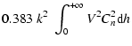
= | ![$\displaystyle 0.0388 \; k^2
\int_0^{+\infty} C_n^2 \; {\rm d\/}h \int\int_{- \infty}^{+\infty} [1-{\rm cos}(2\pi t f_x V)]$](/articles/aa/full/2007/02/aa5788-06/img133.gif) |
|
| = | ![$\displaystyle 0.244 \; k^2
\int_0^{+\infty} C_n^2 \; {\rm d\/}h \int_0^{+\infty} [ 1-J_0(2\pi tVf) ]$](/articles/aa/full/2007/02/aa5788-06/img135.gif) |
||
| (A.7) |
| |
![$\displaystyle \int_0^{\infty} x^{-8/3} \; [ 1 - J_0(\beta x)] \; {\rm d\/}x$](/articles/aa/full/2007/02/aa5788-06/img147.gif) |
||
| = | (A.10) |
| (A.11) |
| (A.12 |
For a single turbulent layer, the piston SF is directly proportional
to
![]() .
Considering the small difference between two
alternative definitions of the average wind speed,
.
Considering the small difference between two
alternative definitions of the average wind speed,
![]() ,
a good approximation for the SF at all time increments will be
,
a good approximation for the SF at all time increments will be
 |
(A.13) |
The temporal power spectrum of the Zernike defocus coefficient a4is given in Conan et al. (1995) as
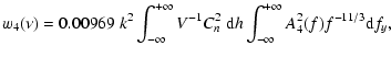 |
(B.1) |
The SF of defocus D4(t) is derived in analogy with the piston SF,
replacing the response A1(f) for piston with A4(f) for
defocus. The coefficient is 2 times smaller because only one aperture
is considered. In analogy with (A.8),
![\begin{displaymath}D_{\varphi}(\vec{r},t) = \langle \left[ \varphi(\vec{r'},t')-\varphi(\vec{r} +\vec{r'}, t + t') \right]^2 \rangle,
\end{displaymath}](/articles/aa/full/2007/02/aa5788-06/img17.gif)
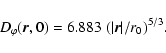
![\begin{displaymath}D_{\varphi,i}(0,t) = 6.883 \; [V(h) t/r_{0,i} ]^{5/3}.
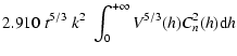
\end{displaymath}](/articles/aa/full/2007/02/aa5788-06/img25.gif)
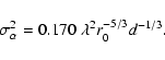
![\begin{displaymath}\overline{V}_p = \left[
\frac{\int_0^{+\infty} V^{p}(h) C_n^...
... }
{\int_0^{+\infty} C_n^2(h) {\rm d}h }
\right] ^{1/p} \cdot
\end{displaymath}](/articles/aa/full/2007/02/aa5788-06/img31.gif)
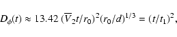
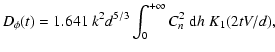
![\begin{displaymath}D_{\phi} (t) \approx 13.76 \; (\overline{V} t /r_0)^2 \;
\left[ 1.17 \; (d/r_0)^2 + (\overline{V} t /r_0)^2 \right]^{-1/6} .
\end{displaymath}](/articles/aa/full/2007/02/aa5788-06/img53.gif)
![\begin{displaymath}\Delta \rho = C_\rho \; a_4 \approx [ 2 \sqrt{3} (1 + \epsilon)/\pi \;
(\lambda/d) ]\; a_4 .
\end{displaymath}](/articles/aa/full/2007/02/aa5788-06/img94.gif)
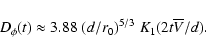
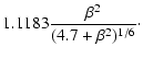
![\begin{displaymath}t_1 \approx 0.284~ C_\rho \Delta t \;
[ D_\rho (2 \Delta t) - D_\rho ( \Delta t)]^{-1/2} .
\end{displaymath}](/articles/aa/full/2007/02/aa5788-06/img104.gif)
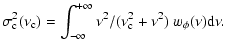
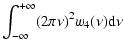
![$\displaystyle D_{\phi} (t) =\int_{-\infty}^{+\infty} 2[1-{\rm cos}(2\pi t \nu)]
\; w_\phi(\nu) \; {\rm d}\nu .$](/articles/aa/full/2007/02/aa5788-06/img127.gif)
![$\displaystyle \int_0^{+\infty} [2 J_1(x)/x ]^2 x^{- 8/3} \; [1-J_0(\beta
x)]\; {\rm d\/}x$](/articles/aa/full/2007/02/aa5788-06/img143.gif)


![$\displaystyle 12\; \int_0^{+\infty} [J_3(x)/x ]^2 x^{- 8/3} \; [1-J_0(\beta
x)]\; {\rm d\/}x$](/articles/aa/full/2007/02/aa5788-06/img170.gif)