All Figures

$\begin{figure} \par\hspace*{4mm}\includegraphics[width=5.7cm,clip]{1350f1a.ps}\v... ...0f1b.ps}\vspace*{5mm} \includegraphics[width=5.6cm,clip]{1350f1c.ps}\end{figure}$ Figure 1: H I observations of NGC 4254 (Phookun et al. 1993). Masks were produced from the data cube, which was smoothed to a resolution of 4'. The spectra were integrated within these masks. Top panel: H I distribution. The contour levels in all images are (0.02, 0.04, 0.06, 0.08, 0.1, 0.2, 0.3, 0.4, 0.5, 0.6, 0.7, 0.8, 0.9, 1.0) times the maximum of the image. Middle panel: velocity field. The contour levels of all images are at 2250-2510 km s^-1 at intervals of 20 km s^-1. Bottom panel: velocity dispersion. The contour levels in all images are at 10-60 km s^-1 in steps of 10 km s^-1.
Open with DEXTER

In the text

$\begin{figure} \par\mbox{\includegraphics[width=7.5cm,clip]{1350f2a.ps}\hspace{2... ...f2c.ps}\hspace{2mm}\includegraphics[width=7.5cm,clip]{1350f2d.ps} } \end{figure}$ Figure 2: Solid lines: Effelsberg 100-m spectra of the four off-center positions. Their locations with respect to the galaxy center are marked on top of each panel. Dashed line: synthesized VLA spectra. Dotted line: 3 $\sigma$ noise levels of the Effelsberg spectra. Velocities are given relative to the systemic velocity of NGC 4254, 2407 km s^-1.
Open with DEXTER

In the text

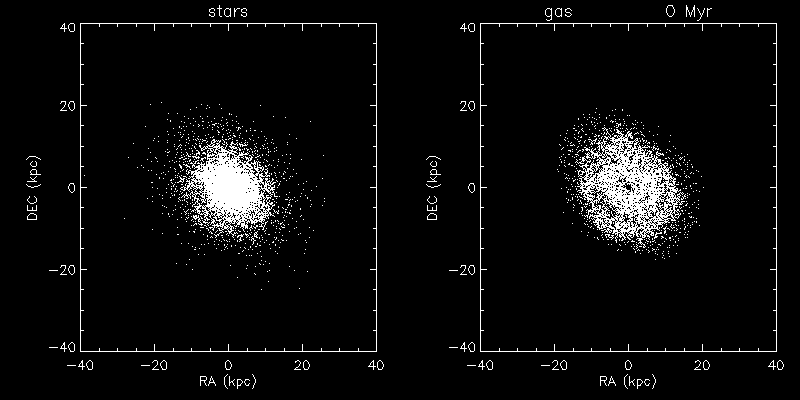
$\begin{figure} \par\includegraphics[width=17.5cm,clip]{1350f3.ps}\end{figure}$ Figure 3: Snapshots of the evolution of the NGC 4254 system model, undergoing only a tidal interaction with another massive Virgo cluster galaxy. The left panels show the stellar disk; the right panels show the gas. The timesteps are marked on the upper right of each panel showing the gas. The center position of the perturbing galaxy is marked as a cross. An animation of this simulation can be found in the electronic version.
Open with DEXTER

In the text

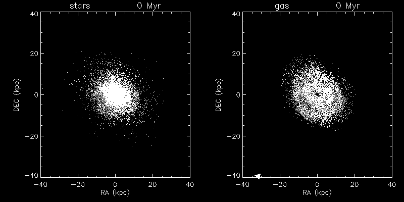
$\begin{figure} \par\includegraphics[width=17.5cm,clip]{1350f4.ps}\end{figure}$ Figure 4: Snapshots of the evolution of the NGC 4254 system model undergoing a tidal interaction with another massive Virgo cluster galaxy, as well as ram pressure stripping. The left panels show the stellar disk; the right panels show the gas. The timesteps are marked on the upper right of each panel showing the gas. The center position of the perturbing galaxy is marked as a cross. The arrow indicates the direction of ram pressure, and the length of the arrow is proportional to its strength. An animation of this simulation can be found in the electronic version.
Open with DEXTER

In the text

$\begin{figure} \par\includegraphics[width=8.15cm,clip]{1350f5a.ps}\vspace*{2mm} \includegraphics[width=7.8cm,clip]{1350f5b.ps}\end{figure}$ Figure 5: The stellar component of NGC 4254. Upper panel: 2MASS K band image (from NED). Lower panel: model distribution for the model with both tidal interaction and ram pressure stripping; snapshot at t=580 Myr.
Open with DEXTER

In the text

$\begin{figure} \par\hspace*{1mm}\includegraphics[width=5.45cm,clip]{1350f6a.ps}\... ...0f6b.ps}\vspace*{5mm} \includegraphics[width=5.8cm,clip]{1350f6c.ps}\end{figure}$ Figure 6: The gaseous component of NGC 4254. Upper panel: model distribution of the H I gas for the model with only a gravitational interaction. Middle panel: model distribution of the H I gas for the model with gravitational interaction plus ram pressure stripping. Lower panel: H I distribution of NGC 4254 observed by Phookun et al. (1993). The contour levels in all images are (0.02, 0.04, 0.06, 0.08, 0.1, 0.2, 0.3, 0.4, 0.5, 0.6, 0.7, 0.8, 0.9, 1.0) times (i) half of the maximum of the image for the models and (ii) the maximum of the image for the H I data.
Open with DEXTER

In the text

$\begin{figure} \par\includegraphics[width=5.3cm,clip]{1350f7a.ps}\vspace*{5mm} \... ...0f7b.ps}\vspace*{5mm} \includegraphics[width=5.3cm,clip]{1350f7c.ps}\end{figure}$ Figure 7: Top panel: model distribution of the H I velocity field for a model of a gravitational interaction alone. Middle panel: distribution of the H I velocity field of the model of a gravitational interaction together with ram pressure. Bottom panel: H I velocity field of NGC 4254 (Phookun et al. 1993). The contour levels of all images are at 2250-2510 km s^-1 at intervals of 20 km s^-1.
Open with DEXTER

In the text

$\begin{figure} \par\includegraphics[width=5.3cm,clip]{1350f8a.ps}\vspace*{5mm} \... ...0f8b.ps}\vspace*{5mm} \includegraphics[width=5.6cm,clip]{1350f8c.ps}\end{figure}$ Figure 8: The gaseous velocity dispersion in NGC 4254. Upperpanel: model gas velocity dispersion map for the model with only a gravitational interaction. Middle panel: model gas velocity dispersion map for the model with both gravitational interaction and ram pressure stripping. Lower panel: H I velocity dispersion map (Phookun et al. 1993). The contour levels in all images are at 10-60 km s^-1 in steps of 10 km s^-1.
Open with DEXTER

In the text

$\begin{figure} \par\includegraphics[width=17.3cm,clip]{1350f9.ps}\end{figure}$ Figure 9: Position-velocity diagrams of 6 selected planes. Contours: H I observations (Phookun et al. 1993). Greyscale: model including ram pressure. Dark regions correspond to regions of low intensity.
Open with DEXTER

In the text

$\begin{figure} \par\includegraphics[width=6.35cm,clip]{1350f10.eps}\end{figure}$ Figure 10: 3D representation of data cubes. The axis of right ascension is indicated. The axis of declination is perpendicular to the image plane. Upper panel: model cube of the simulation including a gravitational interaction alone. Middle panel: model cube of the simulations including a gravitational interaction and ram pressure. Lowerpanel: observed H I data cube (Phookun et al. 1993). The intensity isosurface is at 2 mJy/beam/channel.
Open with DEXTER

In the text

$\begin{figure} \par\includegraphics[width=6.2cm,clip]{1350f11.eps}\end{figure}$ Figure 11: The central H I spectrum of NGC 4254. Upper panel: simulated central H I spectrum at t=580 Myr for the model with only a gravitational interaction. Middle panel: simulated central H I spectrum at t=580 Myr of the model with both gravitational interaction and ram pressure stripping. Lower panel: observations. Solidlines: Effelsberg 100-m single dish spectra of the four off-center positions. Their locations with respect to the galaxy center are marked on top of each panel. Dashed line: synthesized VLA spectrum. Dotted line: 3 $\sigma$ noise level of the 100-m spectrum. Radial velocities are given relative to the systemic velocity of NGC 4254.
Open with DEXTER

In the text

$\begin{figure} \par\includegraphics[width=8.8cm,clip]{1350f12.eps}\end{figure}$ Figure 12: Off-center positions H I spectra of NGC 4254. Solid line: simulated off-center spectra at t=580 Myr for the model with only a gravitational interaction. Dotted line: observed Effelsberg off-center spectra. The locations of the spectra with respect to the galaxy center (see Sect. 3) are marked on top of each panel. Radial velocities are relative to the systemic velocity of NGC 4254.
Open with DEXTER

In the text

$\begin{figure} \par\includegraphics[width=8.8cm,clip]{1350f13.eps}\end{figure}$ Figure 13: Off-center positions H I spectra of NGC 4254. Solid line: simulated off-center spectra at t=580 Myr for the model with both gravitational interaction and ram pressure stripping. Dotted line: observed Effelsberg off-center spectra. The locations of the spectra with respect to the galaxy center (see Sect. 3) are marked on top of each panel. Radial velocities are relative to the systemic velocity of NGC 4254.
Open with DEXTER

In the text

1350f3

1350f4

$\begin{figure} \par\mbox{\includegraphics[width=7.5cm,clip]{1350f2a.ps}\hspace{2... ...f2c.ps}\hspace{2mm}\includegraphics[width=7.5cm,clip]{1350f2d.ps} } \end{figure}$	Figure 2: Solid lines: Effelsberg 100-m spectra of the four off-center positions. Their locations with respect to the galaxy center are marked on top of each panel. Dashed line: synthesized VLA spectra. Dotted line: 3 $\sigma$ noise levels of the Effelsberg spectra. Velocities are given relative to the systemic velocity of NGC 4254, 2407 km s^-1.
Open with DEXTER

$\begin{figure} \par\includegraphics[width=8.15cm,clip]{1350f5a.ps}\vspace*{2mm} \includegraphics[width=7.8cm,clip]{1350f5b.ps}\end{figure}$	Figure 5: The stellar component of NGC 4254. Upper panel: 2MASS K band image (from NED). Lower panel: model distribution for the model with both tidal interaction and ram pressure stripping; snapshot at t=580 Myr.
Open with DEXTER

$\begin{figure} \par\includegraphics[width=17.3cm,clip]{1350f9.ps}\end{figure}$	Figure 9: Position-velocity diagrams of 6 selected planes. Contours: H I observations (Phookun et al. 1993). Greyscale: model including ram pressure. Dark regions correspond to regions of low intensity.
Open with DEXTER

$\begin{figure} \par\includegraphics[width=8.8cm,clip]{1350f12.eps}\end{figure}$	Figure 12: Off-center positions H I spectra of NGC 4254. Solid line: simulated off-center spectra at t=580 Myr for the model with only a gravitational interaction. Dotted line: observed Effelsberg off-center spectra. The locations of the spectra with respect to the galaxy center (see Sect. 3) are marked on top of each panel. Radial velocities are relative to the systemic velocity of NGC 4254.
Open with DEXTER