A&A 429, 963-975 (2005)
DOI: 10.1051/0004-6361:20040480
H. Ozawa - N. Grosso - T. Montmerle
Laboratoire d'Astrophysique de Grenoble, Université Joseph-Fourier, 38041 Grenoble Cedex 9, France
Received 19 March 2004 / Accepted 29 June 2004
Abstract
We observed the main core F of the ![]() Ophiuchi cloud, an active star-forming region located at
Ophiuchi cloud, an active star-forming region located at
![]() pc, using XMM-Newton with an exposure of 33 ks. We detect 87 X-ray sources within the 30
pc, using XMM-Newton with an exposure of 33 ks. We detect 87 X-ray sources within the 30
![]() diameter field-of-view of the EPIC imaging detector array. We cross-correlate the positions of XMM-Newton X-ray sources with previous X-ray, infrared (IR), and optical catalogs: 25 previously unknown X-ray sources are found from our observation; 43 X-ray sources are detected by both XMM-Newton and Chandra; 68 XMM-Newton X-ray sources have 2MASS near-IR counterparts. We show that XMM-Newton and Chandra have comparable sensitivity for point source detection when the exposure time is set to
diameter field-of-view of the EPIC imaging detector array. We cross-correlate the positions of XMM-Newton X-ray sources with previous X-ray, infrared (IR), and optical catalogs: 25 previously unknown X-ray sources are found from our observation; 43 X-ray sources are detected by both XMM-Newton and Chandra; 68 XMM-Newton X-ray sources have 2MASS near-IR counterparts. We show that XMM-Newton and Chandra have comparable sensitivity for point source detection when the exposure time is set to ![]() 30 ks for both. We detect X-ray emission from 7 Class I sources, 26 Class II sources, and 17 Class III sources. The X-ray detection rate of Class I sources is very high (64%), which is consistent with previous Chandra observations in this area. We propose that 15 X-ray sources are new class III candidates, which doubles the number of known Class III sources, and helps to complete the census of YSOs in this area. We also detect X-ray emission from two young bona fide brown dwarfs, GY310 and GY141, out of three known in the field of view. GY141 appears brighter by nearly two orders of magnitude than in the Chandra observation. We extract X-ray light curves and spectra from these YSOs, and find some of them showed weak X-ray flares. We observed an X-ray flare from the bona fide brown dwarf GY310. We find as in the previous Chandra observation of this region that Class I sources tend to have higher temperatures and heavier X-ray absorptions than Class II and III sources.
30 ks for both. We detect X-ray emission from 7 Class I sources, 26 Class II sources, and 17 Class III sources. The X-ray detection rate of Class I sources is very high (64%), which is consistent with previous Chandra observations in this area. We propose that 15 X-ray sources are new class III candidates, which doubles the number of known Class III sources, and helps to complete the census of YSOs in this area. We also detect X-ray emission from two young bona fide brown dwarfs, GY310 and GY141, out of three known in the field of view. GY141 appears brighter by nearly two orders of magnitude than in the Chandra observation. We extract X-ray light curves and spectra from these YSOs, and find some of them showed weak X-ray flares. We observed an X-ray flare from the bona fide brown dwarf GY310. We find as in the previous Chandra observation of this region that Class I sources tend to have higher temperatures and heavier X-ray absorptions than Class II and III sources.
Key words: Galaxy: open clusters and associations: individual: ![]() Ophiuchi cloud - stars: pre-main sequence - stars: low-mass, brown dwarfs - X-rays: stars - infrared: stars
Ophiuchi cloud - stars: pre-main sequence - stars: low-mass, brown dwarfs - X-rays: stars - infrared: stars
Young low-mass stars are known to be ubiquitous X-ray emitters (Montmerle et al.
1993; Feigelson & Montmerle 1999).
Their X-ray luminosities are ![]() 104-105 times higher than that of the present-day Sun.
YSOs are classified from IR and sub-millimeter spectral energy distributions (André & Montmerle 1994) into four classes: Class 0 and Class I protostars, Class II (classical T Tauri stars) and Class III (weak-lined T Tauri stars) sources, interpreted as a time evolution sequence from Class 0 (age
104-105 times higher than that of the present-day Sun.
YSOs are classified from IR and sub-millimeter spectral energy distributions (André & Montmerle 1994) into four classes: Class 0 and Class I protostars, Class II (classical T Tauri stars) and Class III (weak-lined T Tauri stars) sources, interpreted as a time evolution sequence from Class 0 (age
![]() yrs) to Class III (age
yrs) to Class III (age ![]() yrs).
It is generally accepted that enhanced magnetic activity of YSOs produces X-rays emitted by high temperature plasmas as a result of heating by magnetic reconnection events, which is called the solar paradigm because of the analogy with the X-ray emission of the Sun (e.g. as seen with Yohkoh).
yrs).
It is generally accepted that enhanced magnetic activity of YSOs produces X-rays emitted by high temperature plasmas as a result of heating by magnetic reconnection events, which is called the solar paradigm because of the analogy with the X-ray emission of the Sun (e.g. as seen with Yohkoh).
The ![]() Ophiuchi cloud is a well-known nearby active star-forming region at
Ophiuchi cloud is a well-known nearby active star-forming region at
![]() pc,
which has been observed over twenty years by practically all X-ray observatories: Einstein (Montmerle et al. 1983), ROSAT (Casanova 1994; Casanova et al. 1995; Grosso et al. 1997; Grosso 2001), ASCA (Koyama et al. 1994; Kamata et al. 1997; Tsuboi et al. 2000), and Chandra (Imanishi et al. 2001a,b, 2003).
To investigate the YSO X-ray emission in the dense CO core F of the
pc,
which has been observed over twenty years by practically all X-ray observatories: Einstein (Montmerle et al. 1983), ROSAT (Casanova 1994; Casanova et al. 1995; Grosso et al. 1997; Grosso 2001), ASCA (Koyama et al. 1994; Kamata et al. 1997; Tsuboi et al. 2000), and Chandra (Imanishi et al. 2001a,b, 2003).
To investigate the YSO X-ray emission in the dense CO core F of the ![]() Ophiuchi cloud
(Loren et al. 1990), we took with XMM-Newton a 33 ks exposure of this region, as part of the EPIC Guaranteed Time program, and
we report here the results of this observation.
In Sect. 2, we present the observation and data analysis, including source detection,
extraction of X-ray light curves and X-ray spectra from detected sources.
We compare our XMM-Newton results with previously obtained Chandra results in this region in Sect. 3.
We discuss the IR properties of detected sources in Sect. 4.
We present the X-ray detections of young bona fide brown dwarfs in Sect. 5,
and the X-ray properties of Class I-III sources in Sect. 6.
Finally, we summarize all results in Sect. 7.
Ophiuchi cloud
(Loren et al. 1990), we took with XMM-Newton a 33 ks exposure of this region, as part of the EPIC Guaranteed Time program, and
we report here the results of this observation.
In Sect. 2, we present the observation and data analysis, including source detection,
extraction of X-ray light curves and X-ray spectra from detected sources.
We compare our XMM-Newton results with previously obtained Chandra results in this region in Sect. 3.
We discuss the IR properties of detected sources in Sect. 4.
We present the X-ray detections of young bona fide brown dwarfs in Sect. 5,
and the X-ray properties of Class I-III sources in Sect. 6.
Finally, we summarize all results in Sect. 7.
The main (densest) core F of the ![]() Ophiuchi cloud was observed
with XMM-Newton for 33 ks on February 19, 2001 pointing at
Ophiuchi cloud was observed
with XMM-Newton for 33 ks on February 19, 2001 pointing at
![]() and
and
![]()
![]() .
XMM-Newton is the X-ray astronomical observatory of the European Space Agency
which was launched on December 10, 1999.
XMM-Newton has three co-aligned X-ray telescopes with 6
.
XMM-Newton is the X-ray astronomical observatory of the European Space Agency
which was launched on December 10, 1999.
XMM-Newton has three co-aligned X-ray telescopes with 6
![]() -FWHM angular
resolution at 1.5 keV and with large total effective area up to 5000 cm-2 at 1 keV (Jansen et al. 2001).
The European Photon Imaging Camera (EPIC), i.e. two MOS (namely, MOS1 and MOS2) and one PN X-ray CCD arrays,
are placed on each focal plane of the three X-ray telescopes.
EPIC provides imaging capability over a wide field-of-view of 30
-FWHM angular
resolution at 1.5 keV and with large total effective area up to 5000 cm-2 at 1 keV (Jansen et al. 2001).
The European Photon Imaging Camera (EPIC), i.e. two MOS (namely, MOS1 and MOS2) and one PN X-ray CCD arrays,
are placed on each focal plane of the three X-ray telescopes.
EPIC provides imaging capability over a wide field-of-view of 30
![]() diameter, and
spectroscopic capability with moderate spectral resolution (
diameter, and
spectroscopic capability with moderate spectral resolution (![]() 60 eV at 1 keV)
in the 0.2-10.0 keV band. In the present observation,
EPIC was operated with the medium optical blocking filter and in the Full-Frame mode.
60 eV at 1 keV)
in the 0.2-10.0 keV band. In the present observation,
EPIC was operated with the medium optical blocking filter and in the Full-Frame mode.
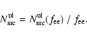
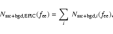
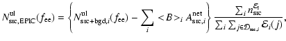
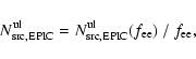
We reduced the data using the XMM-Newton Science Analysis Software (SAS version 5.4). The photon event lists were obtained by running emchain and epchain. We rejected bad pixels, and selected single, double, triple, and quadruple pixel events for MOS, and single and double pixel events for PN using evselect. We excluded the time intervals where the X-ray counts from whole field of view are extremely high, above 4.4 counts s-1 for MOS1 and MOS2, and 20 counts s-1 for PN, indicating a high level of irradiation by solar protons, and hence a high background level on EPIC. The sum of the final good-time-intervals are 31 ks for MOS1, 32 ks for MOS2, and 29 ks for PN.
Figure 1 shows the resulting EPIC image where the MOS1, MOS2, and PN images were corrected for vignetting and co-added. Red, green, and blue colors code the X-ray events in the 0.5-1.0 keV, 1.0-2.4 keV, 2.4-8.0 keV energy bands, respectively. The image is smoothed to enhance the contrast.
We perform the source detection on the individual detector X-ray images, using the standard source detection method of SAS. This method includes 4 steps, heritage of the Einstein and ROSAT source detection algorithms.
As a result of this protocol, we detect in total 87 X-ray sources with a likelihood threshold
above 12, corresponding to the significance of ![]() 4.4
4.4![]() for Gaussian statistics
for Gaussian statistics![]() , within the 30
, within the 30![]() diameter field-of-view of the EPIC detectors. The positions of the detected 87 X-ray sources are indicated in the lower panel of Fig. 1.
Table 1 gives the coordinates, count rates, and the hardness ratios of the detected sources. For convenience, these sources are designated here ROXN-n (for "Rho Oph X-ray sources, Newton, number n'')
diameter field-of-view of the EPIC detectors. The positions of the detected 87 X-ray sources are indicated in the lower panel of Fig. 1.
Table 1 gives the coordinates, count rates, and the hardness ratios of the detected sources. For convenience, these sources are designated here ROXN-n (for "Rho Oph X-ray sources, Newton, number n'')![]() .
The hardness ratios are calculated after the formula
HR = (H - S)/(H + S),
where S and H are counts in the 0.3-2.0 keV, and in the 2.0-8.0 keV energy band, respectively
.
The hardness ratios are calculated after the formula
HR = (H - S)/(H + S),
where S and H are counts in the 0.3-2.0 keV, and in the 2.0-8.0 keV energy band, respectively![]() .
.
The detected sources are cross-correlated with: X-ray source catalogs from Einstein (Montmerle et al. 1983), ROSAT (Casanova et al. 1995; Grosso et al. 2000), ASCA (Kamata et al. 1997), and Chandra (Imanishi et al. 2001a); near-IR source catalogs (e.g. Barsony et al. 1997; 2MASS = Two Micron All-Sky Survey); ISOCAM mid-IR catalog (Bontemps et al. 2001); and an optical catalog (Monet 1996). Table 2 shows the resulting cross-correlation: 62 ROXN sources are identified with previously known X-ray sources, hence we find 25 new X-ray sources from our observation, and 68 ROXN sources have 2MASS near-IR counterparts. Table 2 also lists the IR classifications from Bontemps et al. (2001), or André & Montmerle (1994).
As a result of these cross-identifications, we find 7 Class I sources, 26 Class II sources, and
17 Class III sources. We present 15 previously unknown Class III candidates in Sect. 4.
![\begin{figure}
\par\includegraphics[width=12cm,clip]{0480fig1a.eps}\par\includegraphics[width=12cm,clip]{0480fig1b.eps}
\end{figure}](/articles/aa/full/2005/03/aa0480-04/img19.gif) |
Figure 1:
XMM-Newton observation of the |
We extract background-subtracted X-ray light curves for the ROXN sources.
The X-ray counts are selected from circular regions around the sources where 90% of the X-ray counts
from the sources are included at 1.5 keV![]() .
In crowded regions, we adjust the circle radius to avoid contamination by neighbouring sources.
Background X-ray counts for each source are extracted from annular regions with a 60
.
In crowded regions, we adjust the circle radius to avoid contamination by neighbouring sources.
Background X-ray counts for each source are extracted from annular regions with a 60
![]() inner radius and a 150
inner radius and a 150
![]() outer radius around the sources.
If the annuli contain other X-ray sources, regions within a 40
outer radius around the sources.
If the annuli contain other X-ray sources, regions within a 40
![]() radius
around those sources are excluded from the corresponding annuli.
To avoid decreasing too much the area of the annuli by excluding nearby X-ray sources,
the outer radius was adjusted to keep a constant area for the background extraction region.
radius
around those sources are excluded from the corresponding annuli.
To avoid decreasing too much the area of the annuli by excluding nearby X-ray sources,
the outer radius was adjusted to keep a constant area for the background extraction region.
Since YSOs are known in general to exhibit X-ray flares,
we systematically look for flares in our sources.
We find that nearly half of the sources (40) have enough X-ray counts (N > 150, where N is the sum of MOS1, MOS2 and PN counts)
to search for X-ray flares, using the following method.
We extract X-ray light curves with a uniform reference time binsize. A bin-to-bin variation was then defined to be a flare
if the X-ray counts in a given time bin are 1.5 times higher than at least one of the three preceding bins
with a statistical significance above 4![]() .
We apply this method varying the reference time binsizes from 1000 s to 4000 s by steps of 1000 s, which covers the typical rise times of X-ray flares from YSOs.
To plot the light curves, we use an adaptive binning where the time binsize is tuned to keep a constant number of counts inside each time bin.
This enables us to catch any rapid time variability such as rising phase of X-ray flares.
Depending on the total number of counts, the time bins are tuned so as
to have enough counts in each bin to see the overall time profile properly (see tuning given in Table 3).
.
We apply this method varying the reference time binsizes from 1000 s to 4000 s by steps of 1000 s, which covers the typical rise times of X-ray flares from YSOs.
To plot the light curves, we use an adaptive binning where the time binsize is tuned to keep a constant number of counts inside each time bin.
This enables us to catch any rapid time variability such as rising phase of X-ray flares.
Depending on the total number of counts, the time bins are tuned so as
to have enough counts in each bin to see the overall time profile properly (see tuning given in Table 3).
Figure 2 shows a sample of background-subtracted X-ray light curves. The X-ray flares seen in Fig. 2 show a variety of profiles, broadly characterized by a fast increase and a roughly exponential decay, although some profiles are more symmetrical, with comparatively slow rise and decay phases of similar durations. Contrary to previous X-ray observations which had limited statistics, a "typical'' YSO X-ray flare profile cannot, in general, be reduced to a simple fast rise followed by an exponential decay. Such a complex behavior is also seen in the large X-ray flare database obtained in 40 ks Chandra observations of the Orion Nebula Cluster (Feigelson et al. 2002a).
In our ![]() Oph observations, X-ray flares are detected from 1/4 Class I, 6/13 Class II, and 3/12 Class III sources.
These ratios are 2-3 times lower than those obtained by Chandra (Imanishi et al. 2001a: 14/18 for Class I + Class I candidates, 12/20 for Class II+III), which is to be expected since our XMM-Newton exposure (33 ks) is three times shorter than that of Chandra (100 ks).
The unclassified sources did not show any strong flares.
Oph observations, X-ray flares are detected from 1/4 Class I, 6/13 Class II, and 3/12 Class III sources.
These ratios are 2-3 times lower than those obtained by Chandra (Imanishi et al. 2001a: 14/18 for Class I + Class I candidates, 12/20 for Class II+III), which is to be expected since our XMM-Newton exposure (33 ks) is three times shorter than that of Chandra (100 ks).
The unclassified sources did not show any strong flares.
| Source total counts | Counts inside a time bin |
| 0-500 | 15 |
| 500-1000 | 25 |
| 1000-2000 | 35 |
| 2000-4000 | 50 |
| 4000-6000 | 80 |
| 6000< | 100 |
We now compute background-subtracted X-ray spectra for sources with N > 150 cts (4 Class I,
13 Class II, 12 Class III sources, and 11 unclassified sources).
The way to extract X-ray counts and background counts is the same as for extracting the light
curves![]() .
Since the difference between the responses of MOS1 and MOS2 is not large because they use the same type of CCD array,
we add the MOS1 and MOS2 spectra to improve the statistics, i.e.,
we add the ancillary response files, and average the photon redistribution matrixes of MOS1 and MOS2 weighted by the exposure time of each detector. We treat the PN spectra separately.
The X-ray counts are grouped to obtain spectral bins with 35 and 25 counts
for bright and faint X-ray sources, respectively.
Figure 3 shows examples of the X-ray spectra obtained in our observation.
.
Since the difference between the responses of MOS1 and MOS2 is not large because they use the same type of CCD array,
we add the MOS1 and MOS2 spectra to improve the statistics, i.e.,
we add the ancillary response files, and average the photon redistribution matrixes of MOS1 and MOS2 weighted by the exposure time of each detector. We treat the PN spectra separately.
The X-ray counts are grouped to obtain spectral bins with 35 and 25 counts
for bright and faint X-ray sources, respectively.
Figure 3 shows examples of the X-ray spectra obtained in our observation.
We first fit the separate PN and MOS1+MOS2 spectra with a single temperature thin thermal emission model (MEKAL) combined with an absorption model (WABS)![]() . For sources which do not have enough counts to yield the plasma metal abundance, we fix it to 0.3 solar,
a typical value for YSOs obtained in
. For sources which do not have enough counts to yield the plasma metal abundance, we fix it to 0.3 solar,
a typical value for YSOs obtained in ![]() Oph with ASCA (Kamata et al. 1997) and Chandra (Imanishi et al. 2001a), and also in other star-forming regions. For calculations of emission measures and luminosities, we adopt d = 140 pc, based
on Hipparcos measurements (see discussion in Bontemps et al. 2001), and for consistency with previous ROSAT studies (Grosso et al. 2000).
Oph with ASCA (Kamata et al. 1997) and Chandra (Imanishi et al. 2001a), and also in other star-forming regions. For calculations of emission measures and luminosities, we adopt d = 140 pc, based
on Hipparcos measurements (see discussion in Bontemps et al. 2001), and for consistency with previous ROSAT studies (Grosso et al. 2000).
As a result, we obtain acceptable one-temperature spectral fits for all the sources except for ROXs20A + ROXs20B, SR12A-B and IRS55 (see below).
The values of the fitting parameters are listed in Table 4.
The individual metal abundances obtained from the fits are found to be distributed around 0.3 solar, which is consistent with most existing YSO
X-ray observations.
If we alternatively choose to fix the metal abundance to 0.3 solar for all the sources,
we also obtain acceptable one-temperature fits with better constraints on other spectral parameters
except for the Class I source EL29 (ROXN-22).
EL29 did not show X-ray flares during our observation, whereas it showed X-ray flares during the ASCA and Chandra observations (Kamata et al. 1997; Imanishi et al. 2001a).
We find 1.0 (0.80-1.3) for the metal abundance of EL29 relative to solar,
which is far from the value, ![]() 0.3, observed for the quiescent level by ASCA and Chandra (Kamata et al. 1997; Imanishi et al. 2001a).
Actually, the K
0.3, observed for the quiescent level by ASCA and Chandra (Kamata et al. 1997; Imanishi et al. 2001a).
Actually, the K![]() line from He-like iron ions at 6.7 keV is
clearly seen in the spectra of EL29 (see Fig. 3).
We note a residual in the spectral fitting around 6.4 keV in both PN and MOS1+MOS2, however
adding a Gaussian line at this energy does not change the metallicity at all.
This suggests that the metal abundances of the X-ray emitting plasma in YSOs could be variable.
For example, such metallicity enhancement could be explained by photospheric evaporation produced
by flaring (Güdel et al. 2001).
We list the values of the metal abundances obtained from X-ray spectral fitting
in our observation in Table 4.
line from He-like iron ions at 6.7 keV is
clearly seen in the spectra of EL29 (see Fig. 3).
We note a residual in the spectral fitting around 6.4 keV in both PN and MOS1+MOS2, however
adding a Gaussian line at this energy does not change the metallicity at all.
This suggests that the metal abundances of the X-ray emitting plasma in YSOs could be variable.
For example, such metallicity enhancement could be explained by photospheric evaporation produced
by flaring (Güdel et al. 2001).
We list the values of the metal abundances obtained from X-ray spectral fitting
in our observation in Table 4.
![\begin{figure}
\par\includegraphics[width=14.4cm,clip]{0480fig2.ps}
\end{figure}](/articles/aa/full/2005/03/aa0480-04/img21.gif) |
Figure 2: A sample of X-ray background subtracted light curves of YSOs obtained with XMM-Newton showing variabilities. High background time intervals were suppressed (gaps in the light curve). We use an adaptive binning to keep a constant count number in each bin (see Table 3). X-ray light curves of the bona fide brown dwarfs GY310 and GY141 are shown in Fig. 9. |
![\begin{figure}
\par\includegraphics[angle=270,width=8.8cm,clip]{0480fig3a.ps}\hs...
...ce*{2mm}
\includegraphics[angle=270,width=8.8cm,clip]{0480fig3d.ps}
\end{figure}](/articles/aa/full/2005/03/aa0480-04/img22.gif) |
Figure 3: X-ray spectra of IRS44/YLW16A (Class I), EL29 (Class I), GY314 (Class II), and SR12A-B (Class III) in the quiescent state obtained with XMM-Newton. In each panel, the filled circles and open squares indicate PN and MOS1+MOS2 spectra. The solid lines show the best fit models whose spectral parameters are listed in Table 4. |
Since it is often found that X-ray spectra with low statistics can be modeled by either a single temperature or a two-temperature MEKAL + absorption model, we also test a two-temperature MEKAL + absorption model for all the ROXN sources. The metal abundance is then fixed to 0.3 solar except for EL29. We obtain acceptable two-temperature fits for all the sources except for SR12A-B, but the emission measures of the soft components are either extremely large or very low for most sources. This means that the large absorption of the sources does not allow us to constrain the parameters of the soft component, so that one-temperature fits are sufficient in practice. However, for the bright Class III sources ROXs20A and ROXs20B (i.e., ROXN-27 and ROXN-28, which are spatially resolved but with too few counts, hence we use a circular area encompassing both sources to obtain a spectrum), SR12A-B (ROXN-36) and IRS55 (ROXN-73), two-, three-, and two-temperature MEKAL + absorption models, respectively, are needed to obtain acceptable fits (see Fig. 3).
Chandra observed the ![]() Ophiuchi cloud core F region with an exposure of 100 ks (Imanishi et al. 2001a), although, contrary to our XMM-Newton observations, the pointing was somewhat off-centered with respect to the peak of the CO emission of core F.
Figure 4 shows the XMM-Newton and Chandra X-ray source positions superimposed on the 0.3-8 keV band image obtained by XMM-Newton.
Chandra detected in 100 ks 87 X-ray sources in its field of view (17
Ophiuchi cloud core F region with an exposure of 100 ks (Imanishi et al. 2001a), although, contrary to our XMM-Newton observations, the pointing was somewhat off-centered with respect to the peak of the CO emission of core F.
Figure 4 shows the XMM-Newton and Chandra X-ray source positions superimposed on the 0.3-8 keV band image obtained by XMM-Newton.
Chandra detected in 100 ks 87 X-ray sources in its field of view (17
![]() ). This the same number of sources as in our three times shorter XMM-Newton observations, in a field of view which is nearly four times as large. We shall return to this coincidence below.
In the region covered by the field of view of both observatories, 47 X-ray sources are detected with XMM-Newton and 81 X-ray sources are detected with Chandra, while 43 X-ray sources are detected with both observatories.
). This the same number of sources as in our three times shorter XMM-Newton observations, in a field of view which is nearly four times as large. We shall return to this coincidence below.
In the region covered by the field of view of both observatories, 47 X-ray sources are detected with XMM-Newton and 81 X-ray sources are detected with Chandra, while 43 X-ray sources are detected with both observatories.
Figure 5 shows XMM-Newton vs. Chandra count rates for all these X-ray sources.
Upper limits correspond to the 99.9989% confidence level threshold
(i.e., 4.4![]() level for Gaussian statistics)
for the Chandra sources undetected by XMM-Newton, and for the XMM-Newton sources
undetected by Chandra, using a method explained in Appendix A.
The median of the count rate upper limits of sources detected with only Chandra
is the dotted horizontal line in Fig. 5, which indicates
also the 4.4
level for Gaussian statistics)
for the Chandra sources undetected by XMM-Newton, and for the XMM-Newton sources
undetected by Chandra, using a method explained in Appendix A.
The median of the count rate upper limits of sources detected with only Chandra
is the dotted horizontal line in Fig. 5, which indicates
also the 4.4![]() detection threshold for XMM-Newton.
There is a good correlation between XMM-Newton and Chandra count rates.
The median of the ratios between XMM-Newton and Chandra count rates for X-ray sources detected by both observatories is 6.8, which is indicated by a continuous line in Fig. 5: "the median ratio line''.
Most of the data points are scattered close to this median ratio line.
A few sources display large discrepancies between XMM-Newton and Chandra observations,
which suggests that their X-ray luminosities could have changed due to time
variability.
We checked the two most extreme cases, sources ROXN-33 (GY245) and ROXN-46 (YLW16A), which are far from the median ratio line.
GY245 did not show any flare during the Chandra observation, but showed a flare during the XMM-Newton observation, while YLW16A showed an X-ray flare during the Chandra observation, but did not show any flare during the XMM-Newton observation.
Hence, flaring activity explains well the large apparent discrepancies observed for these two sources.
detection threshold for XMM-Newton.
There is a good correlation between XMM-Newton and Chandra count rates.
The median of the ratios between XMM-Newton and Chandra count rates for X-ray sources detected by both observatories is 6.8, which is indicated by a continuous line in Fig. 5: "the median ratio line''.
Most of the data points are scattered close to this median ratio line.
A few sources display large discrepancies between XMM-Newton and Chandra observations,
which suggests that their X-ray luminosities could have changed due to time
variability.
We checked the two most extreme cases, sources ROXN-33 (GY245) and ROXN-46 (YLW16A), which are far from the median ratio line.
GY245 did not show any flare during the Chandra observation, but showed a flare during the XMM-Newton observation, while YLW16A showed an X-ray flare during the Chandra observation, but did not show any flare during the XMM-Newton observation.
Hence, flaring activity explains well the large apparent discrepancies observed for these two sources.
There is a large difference between the number of X-ray sources detected with XMM-Newton and detected with Chandra in the region common to the field of view of both observatories, which we now seek to explain.
The observation time of Chandra, 100 ks,
is three times longer than that of XMM-Newton, 33 ks.
If the observation time of Chandra had been as short as that of XMM-Newton,
the number of sources detected by Chandra would have been smaller. More precisely,
if we assume that ![]() 6 counts are needed to make a Chandra detection
and that the count rates of the X-ray sources are constant,
in a 33 ks Chandra observation,
only those sources with count rates above 0.18 counts ks-1 would have been detected (see the dotted line in Fig. 5).
Figure 5 shows that most of the 23 X-ray sources detected by Chandra only
with count rates above 0.18 counts ks-1 are distributed well below the median ratio line,
which indicates that these sources probably showed X-ray flares only during the 100 ks Chandra observation,
but could disappear in a shorter, 33 ks observation.
All in all, when the exposure time is set to about 30 ks for both observatories, and taking into account the differences in fields of view and detection thresholds, Chandra and XMM-Newton detect roughly the same
number of sources.
6 counts are needed to make a Chandra detection
and that the count rates of the X-ray sources are constant,
in a 33 ks Chandra observation,
only those sources with count rates above 0.18 counts ks-1 would have been detected (see the dotted line in Fig. 5).
Figure 5 shows that most of the 23 X-ray sources detected by Chandra only
with count rates above 0.18 counts ks-1 are distributed well below the median ratio line,
which indicates that these sources probably showed X-ray flares only during the 100 ks Chandra observation,
but could disappear in a shorter, 33 ks observation.
All in all, when the exposure time is set to about 30 ks for both observatories, and taking into account the differences in fields of view and detection thresholds, Chandra and XMM-Newton detect roughly the same
number of sources.
| Class I | ||||||||
| ROXN | Name | kT |
|
Abundance | E.M. |
|
||
| (1022 cm-2) | (1052 cm-3) | (1029 erg s-1) | ||||||
| (1) | (2) | (3) | (4) | (5) | (6) | (7) | (8) | (9) |
| 22 | EL29 | 4.3(3.6-5.1) | 4.9(4.4-5.3) | 1.0(0.80-1.3) | 16.0(13.6-18.9) | 27.5 | 90.0/ 63.0 | |
| 43 | IRS43/YLW15 | 3.9(3.0-5.3) | 3.3(2.9-3.8) | [0.30] | 13.1(10.2-17.3) | 17.3 | 36.5/ 35.0 | |
| f | 3.2(2.7-3.9) | 4.0(3.5-4.5) | [0.30] | 29.1(22.8-37.0) | 34.8 | 56.3/ 45.0 | ||
| 46 | IRS44/YLW16A | 2.7(2.4-3.1) | 5.3(4.9-5.7) | 0.28(0.19-0.38) | 45.6(38.3-53.9) | 49.7 | 77.0/ 72.0 | |
| 66 | IRS51 | 2.1(1.8-2.8) | 4.2(3.5-4.8) | 0.62(0.27-1.18) | 13.8(10.2-18.5) | 16.2 | 51.7/ 48.0 | |
| Class II | ||||||||
| ROXN | Name | kT |
|
Abundance | E.M. |
|
||
| ID | (1022 cm-2) | (1052 cm-3) | (1029 erg s-1) | |||||
| (1) | (2) | (3) | (4) | (5) | (6) | (7) | (8) | (9) |
| 1 | DoAr25 | 6.4(4.9-8.8) | 1.1(0.96-1.2) | 0.26(0.02-0.51) | 157(141-177) | 247 | 80.1/ 72.0 | |
| 11 | SR24S | 2.3(2.0-2.7) | 1.2(1.0-1.3) | 0.24(0.07-0.43) | 16.3(13.4-19.4) | 15.9 | 107.7/ 75.0 | |
| 18 | WL17 | 2.9(2.0-4.3) | 4.1(3.1-5.2) | [0.30] | 8.4(5.0-14.6) | 9.6 | 27.5/ 19.0 | |
| f | 3.2(2.5-4.2) | 4.5(3.8-5.4) | 0.66(0.31-1.2) | 18.1(13.1-25.7) | 24.8 | 35.4/ 25.0 | ||
| 29 | IRS34 | 1.8(1.1-3.7) | 2.7(1.6-4.4) | [0.30] | 12.8(<41.5) | 11.7 | 4.7/ 5.0 | |
| 30 | WL20 | 2.3(1.8-3.0) | 2.0(1.6-2.4) | [0.30] | 8.1(5.9-11.4) | 8.1 | 16.2/ 17.0 | |
| f | 3.4(2.7-4.5) | 2.0(1.7-2.3) | 0.34(0.04-0.75) | 16.4(13.3-20.2) | 20.4 | 34.7/ 29.0 | ||
| 33 | GY245 | 2.1(1.3-5.0) | 7.7(5.2-11.0) | [0.30] | 4.5(1.5-16.4) | 4.4 | 10.9/ 9.0 | |
| 45 | VSSG25 | f | 2.0(1.6-2.5) | 1.1(0.9-1.4) | [0.30] | 6.3(4.7-8.2) | 5.9 | 29.1/ 24.0 |
| 50 | IRS47 | f | 2.9(1.7-7.4) | 2.3(1.5-3.3) | [0.30] | 7.5(<15.5) | 8.5 | 1.2/ 2.0 |
| 57 | GY292 | 2.3(2.1-2.5) | 1.7(1.5-1.8) | 0.23(0.14-0.36) | 31.2(28.6-35.8) | 30.8 | 159.3/153.0 | |
| 61a | IRS49 | 2.0(1.9-2.2) | 1.6(1.4-1.7) | 0.18(0.08-0.29) | 27.1(23.9-30.7) | 24.1 | 131.1/114.0 | |
| 62 | GY310 | f | 2.5(1.7-3.6) | 0.82(0.59-1.2) | [0.30] | 1.8(1.4-2.4) | 1.9 | 22.4/ 13.0 |
| 63 | GY312 | 2.3(1.7-3.3) | 7.6(6.0-8.7) | [0.30] | 11.4(6.4-22.5) | 11.6 | 25.0/ 17.0 | |
| 65 | GY314 | 2.1(2.0-2.3) | 1.5(1.4-1.6) | 0.16(0.07-0.26) | 31.6(28.4-35.0) | 28.4 | 113.2/113.0 | |
| Class III | ||||||||
| ROXN | Name | kT |
|
Abundance | E.M. |
|
||
| (1022 cm-2) | (1052 cm-3) | (1029 erg s-1) | ||||||
| (1) | (2) | (3) | (4) | (5) | (6) | (7) | (8) | (9) |
| 5 | GY112 | 0.98(0.79-1.1) | 0.36(0.31-0.50) | 0.10(0.06-0.16) | 7.5(6.1-11.8) | 4.3 | 40.9/ 37.0 | |
| 14a | GY193 | 1.27(1.19-1.74) | 0.87(0.56-1.07) | [0.30] | 7.0(4.6-8.2) | 6.0 | 29.4/ 38.0 | |
| 15 | GY194 | 1.5(1.2-1.9) | 0.79(0.6-1.1) | [0.30] | 3.2(2.6-3.9) | 2.8 | 20.7/ 13.0 | |
| 25 | WL19 | 2.5(1.5-4.6) | 8.62(6.0-12.8) | [0.30] | 9.2(3.7-30.7) | 9.8 | 8.4/ 10.0 | |
| 27,28a,b | ROXs20A, ROXs20B | 0.13(0.06-0.18) | 0.42(0.23-1.21) | 4.6 | 59.2/ 40.0 | |||
| 0.66(0.56-0.77) | 1.7(0.8-2.2) | 1.9 | ||||||
| 1.66(1.30-2.29) | 2.8(1.9-3.9) | 2.8 | ||||||
| 32,34,35b,c | WL5,WL4,WL3 | 2.5(2.2-3.0) | 4.7(4.2-5.2) | [0.30] | 60.4(47.4-76.9) | 64.2 | 104.6/ 74.0 | |
| 36 | SR12A-B | 0.11(0.08-0.13) | 0.12(0.08-0.17) | 21.9 | 248.6/205.0 | |||
| 0.25(0.23-0.27) | 18.2(11.1-30.2) | 4.4 | ||||||
| 0.97(0.89-1.03) | 18.6(17.0-25.2) | 11.1 | ||||||
| 3.5(2.5-6.5) | 5.6(3.1-8.3) | 6.5 | ||||||
| f | 0.06(0.03-0.10) | 0.24(0.13-0.55) | 24.0 | 74.0/ 60.0 | ||||
| 0.32(0.28-0.38) | 7.8(4.3-17.1) | 4.2 | ||||||
| 1.22(1.09-1.35) | 15.3(5.5-22.5) | 12.0 | ||||||
| 12.0(>3.1) | 4.9(3.0-10.4) | 7.7 | ||||||
| 39 | GY253 | 1.6(1.4-2.0) | 4.5(3.9-5.2) | [0.30] | 24.9(17.5-34.9) | 22.0 | 57.7/ 52.0 | |
| 52 | BKLT162730-244726 | 1.9(1.3-2.3) | 1.0(0.8-1.5) | [0.30] | 6.6(5.3-11.2) | 6.1 | 44.1/ 43.0 | |
| 72 | GY377 | 1.8(1.1-2.7) | 1.1(0.7-1.8) | [0.30] | 1.7(0.9-3.6) | 1.5 | 7.1/ 11.0 | |
| 73 | IRS55 | 1.1(1.0-1.2) | 0.31(0.20-0.50) | 62.3 | 139.3/141.0 | |||
| 0.64(0.60-0.68) | 46.9(28.0-67.2) | 45.7 | ||||||
| 2.5(2.2-3.0) | 15.7(12.7-19.2) | 16.6 | ||||||
| 76 | GY410 | 1.8(1.3-2.4) | 1.5(1.1-1.9) | [0.30] | 3.8(2.5-5.9) | 3.4 | 8.9/ 23.0 | |
| New Class III candidates | ||||||||
| ROXN | Name | kT |
|
Abundance | E.M. |
|
||
| ID | (1022 cm-2) | (1052 cm-3) | (1029 erg s-1) | |||||
| (1) | (2) | (3) | (4) | (5) | (6) | (7) | (8) | (9) |
| 31 | 16271643-24311 | 4.2(2.2-15.1) | 5.2(3.5-7.4) | [0.30] | 6.1(3.2-14.3) | 8.3 | 25.8/ 26.0 | |
| 41 | GY259 | 3.4(>1.3) | 2.2(1.1-4.5) | [0.30] | 1.9(0.8-6.3) | 2.3 | 0.5/ 2.0 | |
| 44 | GY266 | 2.3(1.1-6.1) | 2.8(1.6-5.0) | [0.30] | 2.4(1.0-8.2) | 2.5 | 7.5/ 6.0 | |
| 53 | GY283 | 1.4(0.5-2.6) | 0.47(0.2-1.5) | [0.30] | 0.5(0.3-3.0) | 0.5 | 2.1/ 4.0 | |
| 58 | GY295 | 1.9(1.2-2.8) | 0.34(0.2-0.6) | [0.30] | 0.7(0.5-0.8) | 0.6 | 12.3/ 11.0 | |
| 77 | BKLT162800-244819 | 0.5(0.4-0.7) | 0.97(0.8-1.1) | [0.30] | 8.7(4.4-17.2) | 7.8 | 24.2/ 25.0 | |
| 78 | GY463 | 1.6(1.2-2.1) | 2.6(2.0-3.4) | [0.30] | 11.0(6.8-20.2) | 9.6 | 16.0/ 20.0 | |
| 86 | BKLT162823-244140 | 4.3(2.2-13.2) | 0.87(0.5-1.3) | [0.30] | 4.0(2.8-6.7) | 5.5 | 9.7/ 9.0 | |
| X-ray sources with no optical or IR counterpart | ||||||||
| ROXN | Name | kT |
|
Abundance | E.M. |
|
||
| ID | (1022 cm-2) | (1052 cm-3) | (1029 erg s-1) | |||||
| (1) | (2) | (3) | (4) | (5) | (6) | (7) | (8) | (9) |
| 51 | ................. | 10.5(>3.9) | 0.92(0.6-1.4) | [0.30] | 2.5(2.0-3.8) | 4.4 | 40.1/ 28.0 | |
| 64 | ................. | 82.4(>20.5) | 2.2(1.7-2.9) | [0.30] | 3.5(2.9-4.1) | 5.5 | 64.5/ 43.0 | |
| 67 | ................. | 3.6(>1.4) | 9.5(4.8-18.0) | [0.30] | 6.7(2.4-46.9) | 8.6 | 25.4/ 29.0 | |
|
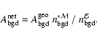
(1) XMM-Newton source ID number, "Rho Oph X-ray sources, Newton''.
(2) The source name from Col. (15) in Table 2.
(3) "f'' means that the X-ray spectra are extracted during the flare phase.
(4-7) The 90% confidence regions are given between parenthesis.
(5) We use WABS for absorption model in XSPEC where standard solar metal abundances are used. The use of revised solar abundances (Holweger 2001; Allende Prieto et al.
2001, 2001) would increase a These sources showed a small flare during the observation, but the X-ray counts in the flares are not sufficient to obtain their spectra. b It is difficult to obtain an individual spectrum without contamination from neighbouring sources. We extracted the X-ray spectrum from a circular region that contains all the sources. c Since the X-ray counts from ROXN-32 is dominant, we put the spectral parameters in the table for Class III. |
In summary, we find that the respective merits of XMM-Newton and Chandra, for the same type of observations (here a typical low-mass star-forming region) are as follows. XMM-Newton has an effective area about three times larger than Chandra,
so that XMM-Newton detects more source counts than Chandra for the same observation time:
as shown in Fig. 5, the XMM-Newton count rate is 6.8 times larger than
the Chandra count rate.
On the other hand, Chandra has a lower background, and a sharper point spread function than XMM-Newton,
which means Chandra suffers less noise than XMM-Newton for point source detection. For relatively short exposures (but typical in a proposal request) of 30 ks, though these values depend on position with respect to the pointing axis,
the signal-to-noise ratios are similar for both observatories.
For longer exposure times, Chandra provides a better detection ability than XMM-Newton, while for shorter exposure times, XMM-Newton provides a slightly better detection ability than Chandra,
because the statistics with Chandra is photon-dominated, while for XMM-Newton it is background-dominated.
Because it detects more photons in a given exposure, XMM-Newton allows a more detailed spectral and time variability analysis for moderately bright sources (above ![]() 150 counts), typical of YSOs, than does Chandra.
150 counts), typical of YSOs, than does Chandra.
![\begin{figure}
\par\includegraphics[angle=270,width=8.8cm,clip]{0480fig4.ps}
\end{figure}](/articles/aa/full/2005/03/aa0480-04/img25.gif) |
Figure 4:
Comparison of source detection between XMM-Newton and Chandra
(Imanishi et al. 2001a).
The background image shows the XMM-Newton image in the 0.3-8 keV energy range smoothed with
a 6
|
ISOCAM provides a reliable classification of YSOs in the ![]() Ophiuchi cloud in terms of Class I or II sources, from the detection of IR excess produced by circumstellar material (Bontemps et al. 2001).
We detect X-rays from 7/11 Class I sources, 25/61 Class II sources, and 14/15 Class III sources in the overlapping region between the field of view of XMM-Newton and the ISOCAM
survey
Ophiuchi cloud in terms of Class I or II sources, from the detection of IR excess produced by circumstellar material (Bontemps et al. 2001).
We detect X-rays from 7/11 Class I sources, 25/61 Class II sources, and 14/15 Class III sources in the overlapping region between the field of view of XMM-Newton and the ISOCAM
survey![]() .
We find a high detection rate for Class I sources (64%), which is higher than that of Class II sources (48%).
The XMM-Newton detection rate of Class I sources is comparable to that obtained from the Chandra observation,
but the detection rate for Class II sources is lower by more than 70% than that obtained by Chandra (Imanishi et al. 2001a).
The Class III sample is biased because these sources were mostly identified by X-rays, which explains why their detection rate is high (93%).
.
We find a high detection rate for Class I sources (64%), which is higher than that of Class II sources (48%).
The XMM-Newton detection rate of Class I sources is comparable to that obtained from the Chandra observation,
but the detection rate for Class II sources is lower by more than 70% than that obtained by Chandra (Imanishi et al. 2001a).
The Class III sample is biased because these sources were mostly identified by X-rays, which explains why their detection rate is high (93%).
Figure 6 is a scatter plot of stellar luminosities (![]() )
vs. extinction (
)
vs. extinction (![]() ), for Class II (filled circles) and Class III sources (open circles) from Bontemps et al. (2001) results. Sources having XMM-Newton X-ray counterparts are indicated by crosses.
Most of the X-ray non-detected Class II sources are distributed in the lower-right region
(low
), for Class II (filled circles) and Class III sources (open circles) from Bontemps et al. (2001) results. Sources having XMM-Newton X-ray counterparts are indicated by crosses.
Most of the X-ray non-detected Class II sources are distributed in the lower-right region
(low ![]() and high
and high ![]() )
of Fig. 6.
Assuming that there is an
)
of Fig. 6.
Assuming that there is an
![]() correlation (see below, Sect. 6),
combined with the high extinction, the X-ray non-detected Class II sources in this region could simply lie below the detection threshold of XMM-Newton (see Grosso et al. 2000) which, as discussed above, is higher than for Chandra.
correlation (see below, Sect. 6),
combined with the high extinction, the X-ray non-detected Class II sources in this region could simply lie below the detection threshold of XMM-Newton (see Grosso et al. 2000) which, as discussed above, is higher than for Chandra.
However, some X-ray non-detected Class II sources, like SR24N , WSB37, and GY3,
are not located in the lower-right region of Fig. 6. This could be explained in two ways.
First, their individual
![]() ratios may be lower than typical ones.
Second, their extinction may be higher than given by the statistical extinctions estimated from the NIR data (Bontemps et al. 2001).
This could happen if the circumstellar disk of
these Class II sources is seen close to edge-on:
in such a case, the central star is not visible, and
we just observe its scattered light so that a statistical value of
ratios may be lower than typical ones.
Second, their extinction may be higher than given by the statistical extinctions estimated from the NIR data (Bontemps et al. 2001).
This could happen if the circumstellar disk of
these Class II sources is seen close to edge-on:
in such a case, the central star is not visible, and
we just observe its scattered light so that a statistical value of ![]() underestimates the real value.
Conversely, two luminous Class III sources with very high extinction, WL5 (ROXN-32) and WL19 (ROXN-25), are located in the upper-right corner of Fig. 6.
Their X-ray spectral fits provide a column density consistent with high absorption (see Table 4).
These two Class III sources are probably located behind the dense core F of cloud. A similar conclusion, in the much wider field of view of ROSAT, was reached for many Class III sources by Grosso et al. (2000).
The correlation between X-ray absorption column density and optical extinction was studied in detail
by Vuong et al. (2003), who compare the gas and dust properties of the dense interstellar matter in
nearby star-forming regions using X-rays from Class III sources.
underestimates the real value.
Conversely, two luminous Class III sources with very high extinction, WL5 (ROXN-32) and WL19 (ROXN-25), are located in the upper-right corner of Fig. 6.
Their X-ray spectral fits provide a column density consistent with high absorption (see Table 4).
These two Class III sources are probably located behind the dense core F of cloud. A similar conclusion, in the much wider field of view of ROSAT, was reached for many Class III sources by Grosso et al. (2000).
The correlation between X-ray absorption column density and optical extinction was studied in detail
by Vuong et al. (2003), who compare the gas and dust properties of the dense interstellar matter in
nearby star-forming regions using X-rays from Class III sources.
![\begin{figure}
\par\includegraphics[width=8.8cm,clip]{0480fig6.ps}
\end{figure}](/articles/aa/full/2005/03/aa0480-04/img30.gif) |
Figure 6: Stellar luminosity vs. extinction for Class II (filled circles) and III (open circles) sources in the ISOCAM survey (Bontemps et al. 2001) and XMM-Newton overlapping area. The sources which have XMM-Newton counterparts are indicated by crosses. The new Class III candidates are indicated by asterisks and are labeled with ROXN numbers of Table 1 and 2. |
![\begin{figure}
\par\includegraphics[width=8.8cm,clip]{0480fig7.ps}
\end{figure}](/articles/aa/full/2005/03/aa0480-04/img31.gif) |
Figure 7: Color-color diagram of the XMM-Newton sources having 2MASS near-IR counterparts. The arrow shows an extinction of 10 mag (Cohen et al. 1981). The intrinsic colors of giants (dotted line) and A0-M6 dwarfs from Bessel & Brett (1988), adapted for the 2MASS photometric system using the 2MASS color transformation (Carpenter 2001; Cutri et al. 2003), are plotted for comparison. The dashed line shows the locus of the intrinsic color classical T Tauri stars (Meyer et al. 1997). Arrows indicate lower limits on J-H when J magnitude is not available. |
Considering that ISOCAM observations of Bontemps et al. (2001) were sensitive enough to detect IR excess from the new X-ray sources found in our observation but did not, these sources are Class III candidates.
There are 37 XMM-Newton X-ray sources without IR classification in Table 2,
18 of which have 2MASS counterparts. With the exception of ROXN-10 (identified with the bona fide brown dwarf GY 141,see below, Sect. 5),
we now check whether the near-IR photometry of these X-ray sources is consistent with that of Class III sources.
![\begin{figure}
\par\includegraphics[width=16cm,clip]{0480fig8.ps}
\end{figure}](/articles/aa/full/2005/03/aa0480-04/img32.gif) |
Figure 8:
Color-magnitude diagram of the XMM-Newton X-ray sources with 2MASS counterparts.
The solid line shows the 1 Myr isochrone for solar metalicity
low-mass stars from 0.02 to 1.00 |
Figure 7 shows the color-color diagram of the XMM-Newton X-ray sources identified with the 2MASS near-IR sources. Class I-III sources and brown dwarfs are indicated by filled diamonds, filled circles, open circles, and open diamonds, respectively; and sources without IR classification are indicated by asterisks labeled with the ROXN numbers of Table 2. As ROXN-31 is too faint to have measurable J and H magnitudes, it is removed from our sample, and 16 unclassified sources are plotted in Fig. 7. For ROXN-41, -44, and -49, only lower limits are available for the J-H color. ROXN-87, corresponding to ROSAT source ROXR-F37, was identified as a foreground F2 V star, HD 148352 (Grosso et al. 2000), which is consistent with its position on the locus of the intrinsic colors (Bessel & Brett 1988). This is also consistent with the fact that its X-ray hardness ratio is -1.0 for MOS1 and -1.0 for MOS2 from Table 1, which means there is no hard X-ray emission above 2 keV. ROXN-47 is also located at the position of a late-type M dwarf without extinction in Fig. 7; its hardness ratio is relatively low, -0.54, -1.00, and -0.76 for MOS1, MOS2, and PN, respectively. We thus consider this source also as a foreground star.
Figure 8 shows the color-magnitude diagrams of H vs. J-H in the left panel,
and ![]() vs.
vs.
![]() in the right panel for XMM-Newton sources having 2MASS counterparts.
(Note that ROXN-31 appears only in the
in the right panel for XMM-Newton sources having 2MASS counterparts.
(Note that ROXN-31 appears only in the ![]() vs.
vs.
![]() diagram since this source is detected only in the
diagram since this source is detected only in the ![]() band.)
We plot for comparison the 1 Myr isochrone (Baraffe et al. 1998) and reddening vectors (Cohen et al. 1981).
The positions of the remaining 15 sources without IR classification are well mixed with those of well-known
Class II and III sources.
Therefore, in view of the absence of IR excess, we propose these 15 X-ray sources as new Class III candidates (labeled "nIII'' in Table 2), therefore doubling the present number of Class III sources in this area.
A spectroscopic follow-up is now needed to determine the effective temperature of these objects, and to put them
in an H-R diagram to confirm their pre-main sequence status.
We estimate stellar luminosities and extinctions of these new Class III candidates using J and H band 2MASS magnitudes (see formulas in Bontemps et al. 2001), and plot them in Fig. 6.
The new Class III candidates are also mixed with the Class II and III sources in Fig. 6.
band.)
We plot for comparison the 1 Myr isochrone (Baraffe et al. 1998) and reddening vectors (Cohen et al. 1981).
The positions of the remaining 15 sources without IR classification are well mixed with those of well-known
Class II and III sources.
Therefore, in view of the absence of IR excess, we propose these 15 X-ray sources as new Class III candidates (labeled "nIII'' in Table 2), therefore doubling the present number of Class III sources in this area.
A spectroscopic follow-up is now needed to determine the effective temperature of these objects, and to put them
in an H-R diagram to confirm their pre-main sequence status.
We estimate stellar luminosities and extinctions of these new Class III candidates using J and H band 2MASS magnitudes (see formulas in Bontemps et al. 2001), and plot them in Fig. 6.
The new Class III candidates are also mixed with the Class II and III sources in Fig. 6.
In summary, we find a high XMM-Newton detection rate for Class I and Class III sources, consistent with the Chandra results, and a lower detection rate for Class II sources. For those sources, the difference is probably due to a combination of high extinction (interstellar + circumstellar) and of lower detection efficiency of XMM-Newton compared with Chandra. We however detect 15 previously unknown X-ray sources, which we propose as new Class III candidates, pending spectroscopic follow-ups to confirm their nature. Our XMM-Newton observations thus allow for a significant improvement of the YSO census in the ![]() Oph cloud core F region (15 new YSOs in addition to a total of 91 previously known from X-ray/IR observations, and a potential doubling of the number of Class III sources).
Oph cloud core F region (15 new YSOs in addition to a total of 91 previously known from X-ray/IR observations, and a potential doubling of the number of Class III sources).
Since ROSAT observations, it is known that young brown dwarfs also emit X-rays (Neuhäuser & Comerón 1998; Neuhäuser et al. 1999; Imanishi et al. 2001a,b; Preibisch & Zinnecker 2001; Mokler & Stelzer 2002; Feigelson et al. 2002b; Tsuboi
et al. 2003). We thus look for X-rays from young bona fide brown dwarfs in our observation, i.e., from young objects with substellar status confirmed by spectroscopy. There are in our field-of-view only three bona fide brown dwarfs![]() : GY202, GY141, and GY310 (Martín et al. 1999; Cushing et al. 2000; Wilking et al. 1999). Bontemps et al. (2001) classified GY310 as Class II, and recently Mohanty et al. (2004) detected it from the ground with Subaru at 8.6 and 11.7
: GY202, GY141, and GY310 (Martín et al. 1999; Cushing et al. 2000; Wilking et al. 1999). Bontemps et al. (2001) classified GY310 as Class II, and recently Mohanty et al. (2004) detected it from the ground with Subaru at 8.6 and 11.7 ![]() m, confirming the presence of significant mid-infrared excess arising from an optically thick, flared dusty disk.
m, confirming the presence of significant mid-infrared excess arising from an optically thick, flared dusty disk.
A low S/N ratio X-ray detection of GY202 was reported by Neuhäuser et al. (1999) from the ROSAT/PSPC pointing observation of Casanova et al. (1995). We find that the identification of this ROSAT/PSPC source with GY202, located 19
![]() away, is dubious because the closest counterpart is in fact WL1, an embedded (
away, is dubious because the closest counterpart is in fact WL1, an embedded (
![]() mag) Class II source (Bontemps et al. 2001), located only 9
mag) Class II source (Bontemps et al. 2001), located only 9
![]() away. Moreover, in spite of the fact that we do not detect WL1, its X-ray emission is confirmed by the Chandra observation (source 13 of Imanishi et al. 2001a) with a luminosity roughly consistent with the ROSAT/PSPC estimate, whereas GY202 is not detected either by Chandra (Imanishi et al. 2001b, 2003) and XMM-Newton (this work).
away. Moreover, in spite of the fact that we do not detect WL1, its X-ray emission is confirmed by the Chandra observation (source 13 of Imanishi et al. 2001a) with a luminosity roughly consistent with the ROSAT/PSPC estimate, whereas GY202 is not detected either by Chandra (Imanishi et al. 2001b, 2003) and XMM-Newton (this work).
A very weak X-ray emission has been reported from GY141 with Chandra (Imanishi et al. 2001b; source BF-S2 in Imanishi et al. 2003): only ![]() 8 X-ray photons were collected during the 100 ks exposure. According to Fig. 5, this low count rate is well below the sensitivity of our XMM-Newton observation. However we detect GY141 (ROXN-10) with a count rate of 7.7 cts ks-1, i.e., at a level
8 X-ray photons were collected during the 100 ks exposure. According to Fig. 5, this low count rate is well below the sensitivity of our XMM-Newton observation. However we detect GY141 (ROXN-10) with a count rate of 7.7 cts ks-1, i.e., at a level ![]() 90 times higher than during the Chandra observation. Although we detect this brown dwarf during a phase of intense X-ray activity, we do not have enough statistics to investigate further this high X-ray state (see its background-subtracted light curve in Fig. 9).
90 times higher than during the Chandra observation. Although we detect this brown dwarf during a phase of intense X-ray activity, we do not have enough statistics to investigate further this high X-ray state (see its background-subtracted light curve in Fig. 9).
X-ray emission was also reported from GY310 with Chandra (Imanishi et al. 2001a,b, 2003).
The Chandra X-ray light curve shows no clear flare, but exhibits aperiodic variability by a factor 2 within the 100 ks exposure,
around ![]()
![]() cts s-1 (Imanishi et al. 2001b). During our observation, GY310 (ROXN-62) displayed an X-ray flare (see Fig. 9). To our knowledge this is the first X-ray flare from a young bona fide brown dwarf with enough counts to derive its X-ray spectrum, due to XMM-Newton's large effective area. The observed count rate with MOS1+MOS2+PN increased from 0.007 cts s-1 to 0.04 cts s-1. The quiescent level gives an equivalent Chandra count rate of
cts s-1 (Imanishi et al. 2001b). During our observation, GY310 (ROXN-62) displayed an X-ray flare (see Fig. 9). To our knowledge this is the first X-ray flare from a young bona fide brown dwarf with enough counts to derive its X-ray spectrum, due to XMM-Newton's large effective area. The observed count rate with MOS1+MOS2+PN increased from 0.007 cts s-1 to 0.04 cts s-1. The quiescent level gives an equivalent Chandra count rate of
![]() cts s-1, consistent with the low value previously observed by Chandra.
We obtain enough X-ray counts from GY310 during the flare to make the spectral analysis presented in
Sect. 2.3 (see Fig. 10 and Table 4).
The derived column density is identical to the one found by Imanishi et al. (2001b). We find a somewhat higher plasma temperature in
our flare observation (2.5 keV, 1.7-3.6 keV), compared to the quiescent Chandra value (1.7 keV, 0.9-2.2 keV), a fairly general characteristic of stellar X-ray flares.
cts s-1, consistent with the low value previously observed by Chandra.
We obtain enough X-ray counts from GY310 during the flare to make the spectral analysis presented in
Sect. 2.3 (see Fig. 10 and Table 4).
The derived column density is identical to the one found by Imanishi et al. (2001b). We find a somewhat higher plasma temperature in
our flare observation (2.5 keV, 1.7-3.6 keV), compared to the quiescent Chandra value (1.7 keV, 0.9-2.2 keV), a fairly general characteristic of stellar X-ray flares.
Similar changes in the level of X-ray activity, X-ray flares, and high plasma temperatures, are ubiquitous in low-mass protostars and T Tauri stars.
This suggests that X-ray emission from brown dwarfs in their early phase of evolution are produced basically by the same solar-like, magnetic activity mechanism at work in low-mass
protostars and T Tauri stars, and more generally in late-type stars, as also noticed in previous studies (Imanishi et al. 2001b; Feigelson et al. 2002b).
![\begin{figure}
\par\includegraphics[width=8.4cm,clip]{0480fig9.ps}
\end{figure}](/articles/aa/full/2005/03/aa0480-04/img37.gif) |
Figure 9: X-ray background subtracted light curves of the young bona fide brown dwarfs GY310 and GY141 obtained with XMM-Newton. High background time intervals were suppressed (gaps in the light curve). We use an adaptive binning to keep a constant count number in each bin (see Table 3). |
![\begin{figure}
\par\includegraphics[angle=270,width=8.8cm,clip]{0480fig10.ps}
\end{figure}](/articles/aa/full/2005/03/aa0480-04/img38.gif) |
Figure 10: X-ray spectra of the young bona fide brown dwarf GY310 during the flare state obtained with XMM-Newton. The filled circles and open squares indicate PN and MOS1+MOS2 spectra. The solid lines show the best fit models whose spectral parameters are listed in Table 4. |
![\begin{figure}
\par\includegraphics[angle=270,width=8.8cm,clip]{0480fig12.ps}
\end{figure}](/articles/aa/full/2005/03/aa0480-04/img40.gif) |
Figure 12:
|
To investigate a possible correlation between the X-ray luminosity ![]() and the stellar luminosity L* of YSOs,
we plot
and the stellar luminosity L* of YSOs,
we plot ![]() vs. L* for Class I-III sources, new Class III candidates, and brown dwarfs in Fig. 11.
We calculate absorption corrected
vs. L* for Class I-III sources, new Class III candidates, and brown dwarfs in Fig. 11.
We calculate absorption corrected ![]() in the 0.5-10 keV band
using the best fit model for the X-ray spectra, which are listed in Table 4.
In Fig. 11, we plot only the ROXN sources which are bright enough to determine their spectral parameters,
except for ROXs20A (ROXN-27), ROXs20B (ROXN-28), WL5 (ROXN-32), WL4 (ROXN-34), and WL3 (ROXN-35), for which the individual X-ray spectra cannot be resolved.
We use L* from Bontemps et al. (2001) for Class I-III sources and brown dwarfs,
and use our estimation of L* for new Class III candidates presented in Sect. 4.
For Class I sources, as the stellar luminosity is unknown because
the central star is invisible due to the remnant dust envelopes,
we use the bolometric luminosity as an upper limit to the stellar luminosity.
The correlation index between
in the 0.5-10 keV band
using the best fit model for the X-ray spectra, which are listed in Table 4.
In Fig. 11, we plot only the ROXN sources which are bright enough to determine their spectral parameters,
except for ROXs20A (ROXN-27), ROXs20B (ROXN-28), WL5 (ROXN-32), WL4 (ROXN-34), and WL3 (ROXN-35), for which the individual X-ray spectra cannot be resolved.
We use L* from Bontemps et al. (2001) for Class I-III sources and brown dwarfs,
and use our estimation of L* for new Class III candidates presented in Sect. 4.
For Class I sources, as the stellar luminosity is unknown because
the central star is invisible due to the remnant dust envelopes,
we use the bolometric luminosity as an upper limit to the stellar luminosity.
The correlation index between ![]() and L* of Class II and III sources in the quiescent state is then -0.08, which indicates a weak correlation.
Indeed the
and L* of Class II and III sources in the quiescent state is then -0.08, which indicates a weak correlation.
Indeed the
![]() ratios show a large spread, from
ratios show a large spread, from
![]() to
to
![]() .
New Class III candidates have similar
.
New Class III candidates have similar ![]() and L* properties as other YSOs,
which is consistent with the assumption of their YSO nature.
and L* properties as other YSOs,
which is consistent with the assumption of their YSO nature.
To compare the characteristics of the X-ray spectra of Class I, II, and III sources,
we show in Fig. 12 the scatter plot of their X-ray determined absorption column density,
![]() ,
vs. plasma temperature, kT.
For ROXN-36 (SR12A-B) and ROXN-73 (IRS55), we calculated the average temperature from the multiple components weighted by their emission measures (see above, Sect. 2.3).
An interesting property emerges from the
,
vs. plasma temperature, kT.
For ROXN-36 (SR12A-B) and ROXN-73 (IRS55), we calculated the average temperature from the multiple components weighted by their emission measures (see above, Sect. 2.3).
An interesting property emerges from the ![]() vs. kT diagram: only a
few data points are seen in the upper-left region and the lower-right region.
The upper-left region is where the X-ray sources have a low plasma temperature and large absorption:
since the soft X-rays from low temperature plasmas are easily absorbed,
it is natural that X-rays should be hard to detect from these sources.
On the other hand, the lower-right region is where the X-ray sources have a high plasma temperature and small absorption, and are thus easy to detect, but this region contains surprisingly few data points.
This could be explained by an intrinsic effect if both the maximum temperature of YSOs and their
circumstellar material causing absorption of X-rays decrease in the course of their evolution.
Class I sources, which are in the early stage of the evolution, are indeed located in the upper-right region of this diagram.
Class II and III sources, which are in a later stage of the evolution, are
located in the region of lower temperature and smaller absorption than Class I sources,
which confirms the results obtained by Chandra (Imanishi et al. 2001a).
There is also a tendency for the temperature and absorption of Class III sources to be lower than those of Class II. We conclude that, although our statistics are still limited, an evolutionary effect seems to be present from the Class I stage (high X-ray temperature, high extinction) to the Class III stage (lower X-ray temperature, lower extinction).
vs. kT diagram: only a
few data points are seen in the upper-left region and the lower-right region.
The upper-left region is where the X-ray sources have a low plasma temperature and large absorption:
since the soft X-rays from low temperature plasmas are easily absorbed,
it is natural that X-rays should be hard to detect from these sources.
On the other hand, the lower-right region is where the X-ray sources have a high plasma temperature and small absorption, and are thus easy to detect, but this region contains surprisingly few data points.
This could be explained by an intrinsic effect if both the maximum temperature of YSOs and their
circumstellar material causing absorption of X-rays decrease in the course of their evolution.
Class I sources, which are in the early stage of the evolution, are indeed located in the upper-right region of this diagram.
Class II and III sources, which are in a later stage of the evolution, are
located in the region of lower temperature and smaller absorption than Class I sources,
which confirms the results obtained by Chandra (Imanishi et al. 2001a).
There is also a tendency for the temperature and absorption of Class III sources to be lower than those of Class II. We conclude that, although our statistics are still limited, an evolutionary effect seems to be present from the Class I stage (high X-ray temperature, high extinction) to the Class III stage (lower X-ray temperature, lower extinction).
The main results of our XMM-Newton 33 ks, 30' diameter observation of the ![]() Ophiuchi cloud core F (i.e., the main molecular core) are as follows:
Ophiuchi cloud core F (i.e., the main molecular core) are as follows:
Acknowledgements
We would like to thank the anonymous referee for comments and suggestions. H.O. acknowledges the Japan Society for the Promotion of Science Overseas Research Fellowship, and support from Conseil National des Astronomes et Physiciens. This paper is based on observations obtained with the XMM-Newton, an ESA science mission with instruments and contributions directly funded by ESA member states and the USA (NASA).
For each instrument, MOS1, MOS2, and PN, we compute with the SAS command eexpmap the
corresponding exposure map with a spatial resolution of
2
![]() for X-ray photons of 1.5 keV energy, and normalize it by its maximum value located on-axis.
The resulting bidimensionnal array,
for X-ray photons of 1.5 keV energy, and normalize it by its maximum value located on-axis.
The resulting bidimensionnal array, ![]() ,
represents the spatial effective area
variations, including CCD gaps, bad pixels, and vignetting, relative to the on-axis value.
From
,
represents the spatial effective area
variations, including CCD gaps, bad pixels, and vignetting, relative to the on-axis value.
From ![]() we define an exposure mask,
we define an exposure mask, ![]() ,
having
,
having
![]() = 0 if
= 0 if
![]() = 0, and
= 0, and
![]() = 1 if
= 1 if
![]()
![]() 0.
This exposure mask shows only CCD gaps.
0.
This exposure mask shows only CCD gaps.
We estimate for each position of undetected Chandra source the local average background.
We extract the event number,
![]() ,
inside the 15
,
inside the 15
![]() -radius disk,
-radius disk,
![]() ,
of geometrical area
,
of geometrical area
![]() centered
on the Chandra source position.
This extraction region contains
centered
on the Chandra source position.
This extraction region contains
![]() sky pixels of
sky pixels of ![]() ,
and
,
and
![]() sky pixels of
sky pixels of ![]() where
where ![]() ,
i.e. which are not CCD gaps. The net pixel area of
,
i.e. which are not CCD gaps. The net pixel area of
![]() is:
is:
 |
(A.1) |
 |
(A.2) |
Then we compute the PSF radius encircling
![]() of the PSF
energy,
of the PSF
energy,
![]() ,
using the radial average of the calibration images in the CCF.
We extract the event number,
,
using the radial average of the calibration images in the CCF.
We extract the event number,
![]() ,
within
the
,
within
the
![]() -radius disk,
-radius disk,
![]() ,
of geometrical area
,
of geometrical area
![]() centered on the Chandra source position.
These counts are the sum of background and source
counts,
centered on the Chandra source position.
These counts are the sum of background and source
counts,
![]() and
and
![]() ,
respectively.
The extraction region
,
respectively.
The extraction region
![]() contains
contains
![]() sky pixels of
sky pixels of ![]() ,
and
,
and
![]() sky pixels of
sky pixels of ![]() where
where ![]() .
The net pixel area of
.
The net pixel area of
![]() is:
is:
 |
(A.3) |
 |
(A.4) |
The upper limit on the total source count is therefore:
 |
(A.5) |
We compute the count rate upper limit for the sum of the MOS1, MOS2, and PN data, the so-called
EPIC instrument,
![]() ,
using this set of straightforward formulae using
the previous notation, where
,
using this set of straightforward formulae using
the previous notation, where
![]() :
:
 |
(A.6) |
 |
(A.7) |
 |
(A.8) |
 |
(A.9) |
We obtained the level 2 data of the Core F observation of the ![]() Ophiuchi dark cloud
(sequence number 200060, observation ID 635) from the Chandra data
archive
Ophiuchi dark cloud
(sequence number 200060, observation ID 635) from the Chandra data
archive![]() .
We computed the exposure map with a resolution of 4
.
We computed the exposure map with a resolution of 4
![]() for X-ray photons of 1.5 keV energy,
and normalized it by its maximum value (on-axis),
from which we derived an exposure mask.
We proceeded as for XMM-Newton data, using for the PSF radius encircling 50% of the PSF
energy the formula given by Feigelson et al. (2002b):
for X-ray photons of 1.5 keV energy,
and normalized it by its maximum value (on-axis),
from which we derived an exposure mask.
We proceeded as for XMM-Newton data, using for the PSF radius encircling 50% of the PSF
energy the formula given by Feigelson et al. (2002b):
![]() ,
where
,
where ![]() is the off-axis angle in arcmin.
is the off-axis angle in arcmin.
We note that for Chandra data, due to the large satellite wobble, bad pixels and CCD gaps
are smoothed in the exposure map and they do not produce holes with sharp edges, hence with the above notation we have
![]() .
By combining (1)-(3), we find a formula identical to the formula (6) of Feigelson et al. (2002b)
when replacing the 90% upper limit count by the observed count.
.
By combining (1)-(3), we find a formula identical to the formula (6) of Feigelson et al. (2002b)
when replacing the 90% upper limit count by the observed count.
To check the reliability of the X-ray derived values of ![]() ,
we plot the
,
we plot the ![]() values determined by Chandra vs. those determined by XMM-Newton for
the X-ray sources with spectral fitting data (see Table 4) in the overlapping field-of-views of the two satellites (see Fig. B.1).
The best fit value of the ratio of the
values determined by Chandra vs. those determined by XMM-Newton for
the X-ray sources with spectral fitting data (see Table 4) in the overlapping field-of-views of the two satellites (see Fig. B.1).
The best fit value of the ratio of the ![]() values from Chandra and XMM-Newton obtained from a linear fit is 0.96 (0.93-0.99, 90% confidence region),
indicating that both determinations of
values from Chandra and XMM-Newton obtained from a linear fit is 0.96 (0.93-0.99, 90% confidence region),
indicating that both determinations of ![]() values are consistent to better than 10%.
values are consistent to better than 10%.
Uncertainties in the X-ray-derived ![]() values were discussed for both Chandra and XMM-Newton in Vuong et al. (2003).
They showed that the use of the recently-revised solar abundances (Holweger 2001; Allende Prieto
et al. 2001, 2002) in X-ray spectral fitting increases
values were discussed for both Chandra and XMM-Newton in Vuong et al. (2003).
They showed that the use of the recently-revised solar abundances (Holweger 2001; Allende Prieto
et al. 2001, 2002) in X-ray spectral fitting increases ![]() values by
values by ![]() 20%.
Both in the X-ray spectral fitting by Chandra (Imanishi et al. 2001a) and by XMM-Newton (this work, see Sect. 2.3), the
20%.
Both in the X-ray spectral fitting by Chandra (Imanishi et al. 2001a) and by XMM-Newton (this work, see Sect. 2.3), the ![]() values were determined using the WABS absorption model in XSPEC where solar standard metal abundances are used.
If the abundance effect shown by Vuong et al. (2003) is taken into account, all
the
values were determined using the WABS absorption model in XSPEC where solar standard metal abundances are used.
If the abundance effect shown by Vuong et al. (2003) is taken into account, all
the ![]() values derived by Chandra and XMM-Newton would increase and all the data points in
Fig. B.1 would move towards the upper-right direction by
values derived by Chandra and XMM-Newton would increase and all the data points in
Fig. B.1 would move towards the upper-right direction by ![]() 20% along the diagonal.
20% along the diagonal.
![\begin{figure}
\par\includegraphics[angle=90,width=8.8cm,clip]{0480fig5.ps}
\end{figure}](/articles/aa/full/2005/03/aa0480-04/img26.gif)
![\begin{figure}
\par\includegraphics[angle=270,width=8.8cm,clip]{0480fig11.ps}
\end{figure}](/articles/aa/full/2005/03/aa0480-04/img39.gif)
![\begin{figure}
\par\includegraphics[angle=270,width=8.8cm,clip]{0480figb1.ps}
\end{figure}](/articles/aa/full/2005/03/aa0480-04/img80.gif)