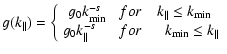
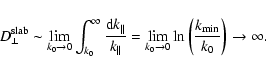
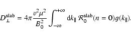
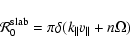
A&A 420, 821-832 (2004)
DOI: 10.1051/0004-6361:20034470
Quasilinear perpendicular diffusion of cosmic rays in weak
dynamical turbulence![[*]](/icons/foot_motif.gif)
A. Shalchi 1,2 - R. Schlickeiser 1
1 - Institut für Theoretische Physik, Lehrstuhl IV:
Weltraum- und Astrophysik, Ruhr-Universität Bochum,
44780 Bochum, Germany
2 -
Now at: Bartol Research Institute, University of Delaware,
Newark, DE 19716, USA
Received 7 October 2003 / Accepted 4 March 2004
Abstract
The quasilinear calculation of perpendicular diffusion of cosmic ray
particles for
weak dynamical magnetic turbulence of arbitrary geometry is presented.
Starting from the equations of motion, a detailed point-by-point
derivation of quasilinear
Fokker-Planck coefficients is given. It is shown that,
to have
diffusive behaviour of the
Fokker-Planck coefficients, the existence of a finite
correlation time of the magnetic fluctuations is essential.
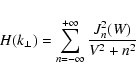
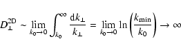
From the perpendicular Fokker-Planck coefficient  ,
the
perpendicular spatial
diffusion coefficient
,
the
perpendicular spatial
diffusion coefficient
 and the associated perpendicular
mean free path
and the associated perpendicular
mean free path
 are calculated
for the damping model of dynamical magnetic turbulence and three
different turbulence geometries: slab, 2D and composite
turbulence.
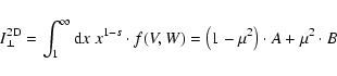
Explicit analytical expressions for the perpendicular transport
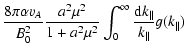
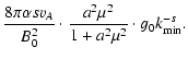
parameters of electrons and
protons are given for realistic heliospheric plasma parameters.
By comparing with our previous determination of the parallel transport
parameters,
the variation of the ratio of mean free paths
are calculated
for the damping model of dynamical magnetic turbulence and three
different turbulence geometries: slab, 2D and composite
turbulence.
Explicit analytical expressions for the perpendicular transport
parameters of electrons and
protons are given for realistic heliospheric plasma parameters.
By comparing with our previous determination of the parallel transport
parameters,
the variation of the ratio of mean free paths
 with particle rigidity
for the three turbulence models is investigated. The comparison of
these predictions with
future accurate experimental determinations of the ratio of mean free
paths will allow conclusions on the nature of interplanetary magnetic
turbulence.
with particle rigidity
for the three turbulence models is investigated. The comparison of
these predictions with
future accurate experimental determinations of the ratio of mean free
paths will allow conclusions on the nature of interplanetary magnetic
turbulence.
Key words: ISM: cosmic rays - plasmas - turbulence - diffusion - Sun:
particle emission
The knowledge of transport parameters of energetic charged particles in
turbulent magnetized cosmic plasmas is a key
problem of cosmic ray astrophysics and space physics.
Of particular interest is the diffusion tensor for particle transport
parallel and perpendicular to the ordered
magnetic field which controls e.g. the penetration and modulation of
low-energy cosmic rays in the heliosphere,
the confinement and escape of galactic cosmic rays from the Galaxy, and
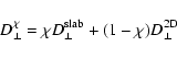
the efficiency of diffusive
shock acceleration mechanisms.
Although the perpendicular diffusion coefficient plays an essential
role in these
studies, a rigorous theoretical treatment in the quasilinear limit of
weak turbulence and for
dynamical magnetic turbulence currently is not available in the
literature.
Available numerical studies (Michalek & Ostrowski 1998; Giacalone &
Jokipii 1999;
Mace et al. 2000; Michalek 2001) are restricted to
magnetostatic turbulence.
It is the purpose of the present paper to provide the quasilinear
calculation of perpendicular
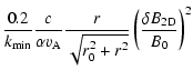
diffusion for weak dynamical magnetic turbulence of arbitrary geometry.
Recently (Shalchi & Schlickeiser 2003 - hereafter referred to SS03) we
calculated
the parallel mean free path of cosmic ray particles in the composite
model and the
damping model of dynamical magnetic turbulence (Bieber et al. 1994)
using the quasilinear
theory (QLT) of particle transport. Here, with the same quasilinear
approximation we
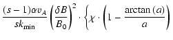
calculate the relevant Fokker-Planck coefficients and transport
parameters for
perpendicular diffusion.
In Sect. 2 we derive and discuss general expressions for the both
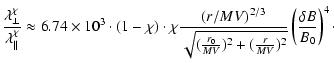
Fokker-Planck
coefficients DXX and DYY, which control the perpendicular
cosmic
ray transport. In Sect. 3 we calculate the Fokker-Planck coefficients
for three
different turbulence geometries: pure slab-, pure 2D- and composite
geometry.
With these results it is possible to calculate the spatial diffusion
coefficient
and the mean free path for perpendicular diffusion (Sect. 4).
In Sect. 5 we use the general results of Sect. 4 to calculate the
perpendicular
diffusion coefficient and the perpendicular mean free path for specific
heliospheric plasma
parameters. Moreover, we calculate the ratio
and compare it with
observations.
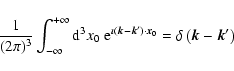
The starting point for the derivation of the quasilinear perpendicular
spatial
diffusion coefficient
are the random parts of the
Lorentz force for the
coordinates X and Y of
the guiding center (see Schlickeiser 2002 - Eqs. (S-12.1.9d)
and (S-12.1.9e)).
For purely magnetic fluctuations these read
 |
|
|
(1) |
 |
|
|
(2) |
In these both equations we used the pitch-angle cosine  ,
the
particle speed v,
the gyrophase
,
the
particle speed v,
the gyrophase  ,
the magnetic background field B0 and the
turbulent fields
in helical coordinates
,
the magnetic background field B0 and the
turbulent fields
in helical coordinates
 and
and
 .
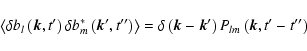
These random force terms determine the corresponding
Fokker-Planck coefficients (see Hall & Sturrock 1968)
.
These random force terms determine the corresponding
Fokker-Planck coefficients (see Hall & Sturrock 1968)
| DXX |
= |
 |
|
| DYY |
= |
 |
(3) |
which have to be calculated from the ensemble-averaged first-order
corrections to the
particle orbits in the weakly turbulent magnetic field. In this
section, we go through
this derivation point by point. We explicitly calculate the
Fokker-Planck
coefficient DXX; the coefficient DYY is calculated in
analogous way: we will
give the final result but leave the details as exercise to the
interested reader.
The perpendicular spatial diffusion coefficient
and the corresponding perpendicular mean free path
are given by the -average (see Schlickeiser 2002)
The quasilinear approximation is achieved by replacing
in the Fourier transform of the fluctuating magnetic field
the true particle orbit
 by the unperturbed orbit
 ,
resulting in
,
resulting in
 |
(6) |
and (see Eq. (S-12.2.3a))
respectively, where
 denotes the initial
(t=0)
position of the cosmic ray particle. In the last both equations we used
the gyrofrequency
denotes the initial
(t=0)
position of the cosmic ray particle. In the last both equations we used
the gyrofrequency  and the
parameter
and the
parameter
 .
For the
wavevector
.
For the
wavevector  we used
cylindrical coordinates:
we used
cylindrical coordinates:
With these approximations the equation of motion (1) becomes
where
 |
(10) |
If we integrate Eq. (9) over time we obtain with the initial
condition
X(t=0)=X0 for the displacement
 :
:
Upon multiplying Eq. (11) with its complex conjugate we find for
the square of the displacement
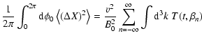
Now we use that the turbulence fields are homogenously distributed, and
average Eq. (12) over the initial spatial position of the cosmic
ray particles using
 |
(13) |
implying that turbulence fields at
different wavevectors are uncorrelated. The respective average of Eq. (12)
with
 |
(14) |
then yields after performing the
 -integration
Next we assume that the initial phase  of the cosmic ray
particle is a random variable
that can take on any value between 0 and
of the cosmic ray
particle is a random variable
that can take on any value between 0 and  .
The averaging of
Eq. (15) over
then represents exactly the ensemble-averaging over the turbulent
magnetic field. Using
.
The averaging of
Eq. (15) over
then represents exactly the ensemble-averaging over the turbulent
magnetic field. Using
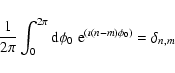 |
(16) |
the double sum over n and m in Eq. (16) is reduced to a
single sum. We obtain after some straightforward resumming
To proceed we have to specify the time behaviour of the magnetic field
correlation tensor
 .
We assume that all tensor components
have the same temporal
behaviour, i.e.
.
We assume that all tensor components
have the same temporal
behaviour, i.e.
 |
(18) |
This assumption allows us to disentangle the time and
-integrations in Eq. (17). We find
where we defined the so-called resonance function
 |
(20) |
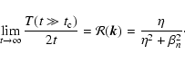
The behaviour of the function T for large times determines whether
perpendicular cosmic ray transport is diffusive
(i.e.
 ),
subdiffusive (
),
subdiffusive (
 ,
s<1), or
superdiffusive (i.e.
,
s>1),
respectively.
We demonstrate here that diffusive perpendicular transport always
exists under two conditions:
,
s<1), or
superdiffusive (i.e.
,
s>1),
respectively.
We demonstrate here that diffusive perpendicular transport always
exists under two conditions:
- (a)
- the time correlation function F of magnetic turbulence
depends only on the absolute value of the difference
t'-t'', i.e.
 ;
;
- (b)
- there exists a finite correlation time
 ,
that can be wave-number dependent,
beyond which the correlation function F falls to a negligible
magnitude.
,
that can be wave-number dependent,
beyond which the correlation function F falls to a negligible
magnitude.
As one particular choice of the correlation function F we consider
here the exponential function
This choice is justified in case of plasma wave turbulence
(Schlickeiser 2002, Sect. 12.2.2) where  then has to be identified with
the wave damping rate. Another choice in accord with the general
requirements (a) and (b) would be the damping model of dynamical
magnetic turbulence and
the random sweeping turbulence, discussed by Bieber et al. (1994).
With Eq. (21) inserted into Eq. (20) we obtain
then has to be identified with
the wave damping rate. Another choice in accord with the general
requirements (a) and (b) would be the damping model of dynamical
magnetic turbulence and
the random sweeping turbulence, discussed by Bieber et al. (1994).
With Eq. (21) inserted into Eq. (20) we obtain
 |
(22) |
The t''-integration is now split into the two intervals
(i)
 where
|t'-t''|=t'-t'',
where
|t'-t''|=t'-t'',
and
(ii)
 where
|t'-t''|=t''-t',
where
|t'-t''|=t''-t',
so that
After changing integration variables to
s1=t'-t'' and
s2=t''-t' in the first and second t''-integral, respectively, we
obtain after straightforward algebra
First of all, we note that for times much larger than the correlation
time,
 ,
the resonance function (24)
approaches the limit
,
the resonance function (24)
approaches the limit
 |
(25) |
proving that the transport indeed is diffusive for large times.
According to the definition (3) we
have to take the limit
 |
(26) |
With Eq. (19) the Fokker-Planck coefficient DXX then
becomes
This completes the derivation of the Fokker-Planck coefficient DXX
for general turbulence geometries.
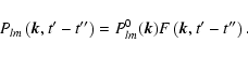
For further reduction, the turbulence geometry has to be specified via
the tensor
 .
This will be the subject of the next sections.
It is instructive to inspect several special cases of the resonance
function (24).
For an infinitely large correlation time
.
This will be the subject of the next sections.
It is instructive to inspect several special cases of the resonance
function (24).
For an infinitely large correlation time
 ,
corresponding to
,
corresponding to
 ,
Eq. (24) reduces to
,
Eq. (24) reduces to
![\begin{displaymath}T(\eta =0)={2[1-\cos \beta _nt]\over \beta _n^2}={4\sin ^2(\beta
_nt/2)\over \beta _n^2}\cdot
\end{displaymath}](/articles/aa/full/2004/24/aa0470/img155.gif) |
(28) |
As has been noted before by Jaekel & Schlickeiser (1992) for large t
this resonance function approaches
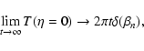 |
(29) |
yielding again diffusive behaviour, but in this case with the resonance
function
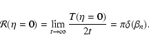 |
(30) |
This is fully consistent with Eq. (26), because of the same limit
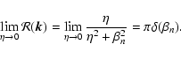 |
(31) |
The use of the resonance function (30) is only problematic in
cases where
 ,
as one
encounters for 2D turbulence, see below (Sect. 4.2).
In this case it is appropriate to go back
to the general resonance function (24) which in the limit
,
as one
encounters for 2D turbulence, see below (Sect. 4.2).
In this case it is appropriate to go back
to the general resonance function (24) which in the limit
 is
is
![\begin{displaymath}T(\beta _n=0)\to {2t\over \eta }\left[1-{1-{\rm e}^{-\eta t}\over \eta
t}\right].
\end{displaymath}](/articles/aa/full/2004/24/aa0470/img161.gif) |
(32) |
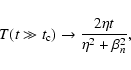
For large times
 this resonance function approaches
 ,
indicating that the motion is still diffusive and that the resonance
condition is
,
indicating that the motion is still diffusive and that the resonance
condition is
 |
(33) |
which agrees with the corresponding limit of Eq. (26).
As an aside, we note that in the limit
and ,
the resonance functions (24) and (32) both imply
superdiffusive behaviour,
 |
(34) |
We conclude, that in order to have diffusive behaviour of the
Fokker-Planck coefficients in all limiting cases the existence of a
finite correlation time of the magnetic fluctuations, i.e. condition
(b) of Sect. 2.7, is essential.
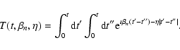
By repeating the analysis for the equation of motion (2) we
obtain in analogy to Eq. (27)
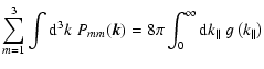
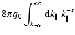
For the sum of Fokker-Planck coefficients we then find
Now we use the general results for the perpendicular Fokker-Planck
coefficient
of the last Sect. (see Eq. (36)) to calculate
for
different turbulence
geometries. To do this we have to specify the tensor Plm0.
According to
Matthaeus & Smith (1981) the components of this tensor can be written
as
![\begin{displaymath}P_{lm}^0 = g(k_{\perp}, k_{\parallel}) \cdot \left[\delta _{l...
..._m \over k^2} + i \sigma \epsilon _{lmn} {k_n \over k}\right],
\end{displaymath}](/articles/aa/full/2004/24/aa0470/img181.gif) |
(37) |
with the magnetic helicity  .
The function
.
The function
 determines
different turbulence geometries. We will consider two geometries
explicitly
in the following:
determines
different turbulence geometries. We will consider two geometries
explicitly
in the following:
(a) slab turbulence, and
(b) pure 2D geometry.
With the results of these both geometries we are also able to calculate
the perpendicular Fokker-Planck
coefficient for composite geometry which is the subject of Sect. 3.3.
For our calculations in
both geometries we use the damping model of the dynamical magnetic
turbulence.
In the case of pure slab geometry Eq. (37) becomes to
![\begin{displaymath}P_{lm}^0 = g(k_{\parallel}) {\delta(k_{\perp}) \over k_{\perp...
...er k^2} + i \sigma \epsilon _{lmn}
{k_n
\over k} \right]\cdot
\end{displaymath}](/articles/aa/full/2004/24/aa0470/img184.gif) |
(38) |
Consequently, many components of the tensor
Plm0 are zero
except
| PRR 0 |
= |
 |
|
| PLL 0 |
= |
 |
(39) |
Therefore we obtain for the perpendicular Fokker-Planck coefficient for
slab
geometry
 = =  |
(40) |
If we use the damping model of dynamical magnetic turbulence we have
according to Eq. (26)
 |
(41) |
because (Bieber et al. 1994)
 |
(42) |
Using
 we find for the Fokker-Planck coefficient
 |
(43) |
To proceed further, we have to specify
the form of the power spectrum
 .
Here we
use a power-law spectrum with a sharp cut-off at small wavenumbers:
.
Here we
use a power-law spectrum with a sharp cut-off at small wavenumbers:
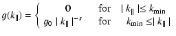 |
|
|
(44) |
with 1<s<2. In Appendix C we discuss the results for
a power spectrum with finite wave power at small wavennumbers (see
Bieber et al. 1994;
Teufel & Schlickeiser 2003, SS03) which causes a divergence problem.
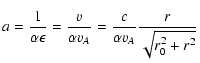
It is convenient to express our results in terms of the
following parameters:
with the cosmic ray particle's rigidity
 and the constant
 .
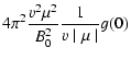
The Fokker-Planck coefficient (43) then becomes
.
The Fokker-Planck coefficient (43) then becomes
Expressing the constant g0 in terms of the total fluctuating
magnetic field strength of the slab component,
yields
 |
(48) |
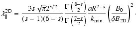
For 2D geometry
![\begin{displaymath}P_{lm}^0 = g(k_{\perp}) {\delta(k_{\parallel}) \over k_{\perp...
...\over k^2} + i \sigma \epsilon _{lmn}
{k_n
\over k} \right]
,
\end{displaymath}](/articles/aa/full/2004/24/aa0470/img210.gif) |
(49) |
yielding for the individual non-zero components
With these components the
Fokker-Planck coefficient (36) reduces to
For the calculations in the 2D-geometry we use
 |
(52) |
implying for the resonance function (21)
 |
(53) |
For vanishing magnetic helicity  the
Fokker-Planck coefficient (51) then becomes
the
Fokker-Planck coefficient (51) then becomes
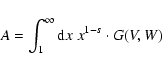
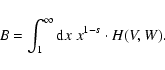
Two of the k-integrations can be readily performed, so that
which can be written as
 |
(56) |
where for brevity we introduced the functions
 |
(57) |
 |
(58) |
and
 |
(59) |
with
 |
(60) |
 |
(61) |
and
 .
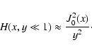
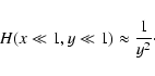
In Appendix A we derive the following approximations for the functions
G and H:
.
In Appendix A we derive the following approximations for the functions
G and H:
For a simple power law turbulence spectrum with sharp low-wavenumber
cut-off as in Sect. 3.1,
but now in  ,
we obtain for the
Fokker-Planck coefficient (54)
,
we obtain for the
Fokker-Planck coefficient (54)
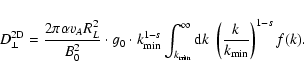 |
(64) |
Again, the constant g0 can be expressed in terms of the total
fluctuating magnetic field strength in the 2D component:
so that
 |
(66) |
with
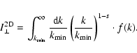 |
(67) |
Substituting
 we find
 |
(68) |
in terms of the integrals
 |
(69) |
and
 |
(70) |
In Eqs. (68)-(70) we use
 |
(71) |
and
We obtain for G and H
Using Eqs. (73) and (74) to calculate the integrals
A and B we obtain the approximations shown in Table 1.
3.3 The Fokker-Planck coefficient in the composite slab/2D geometry is
simply additive and can be written as
 |
(75) |
If we replace
 in Eq. (48) and
 in Eq. (66) by the total turbulence
  we find
 |
(76) |
where the parameter
 |
(77) |
measures the relative strength of slab turbulence with respect to the total
turbulence
 .
.
With the results of the last subsections (Eqs. (48) and (66)) we immediately
determine the Fokker-Planck coefficient in the composite model:
 = =  |
(78) |
with
 of Eq. (68).
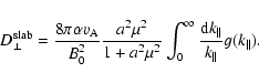
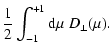
In this section we calculate the perpendicular spatial diffusion
coefficient
and the corresponding perpendicular mean free path for slab geometry.
Using the perpendicular Fokker-Planck coefficient (48) in Eq.
(4) we obtain
of Eq. (68).
In this section we calculate the perpendicular spatial diffusion
coefficient
and the corresponding perpendicular mean free path for slab geometry.
Using the perpendicular Fokker-Planck coefficient (48) in Eq.
(4) we obtain
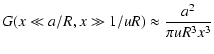
which can be approximated as
For large values of  the spatial diffusion coefficient is
independent of a and therefore independent of the rigidity, whereas
for small
values
the spatial diffusion coefficient is
independent of a and therefore independent of the rigidity, whereas
for small
values  it increases
 below
below  .
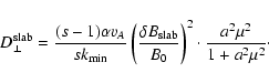
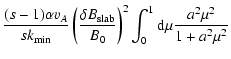
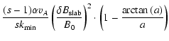
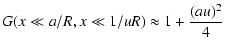
The corresponding perpendicular mean free path is
.
The corresponding perpendicular mean free path is
 = =  |
(81) |
with the approximative behaviour
 |
|
|
(82) |
For large values of
the mean free path decreases proportional
to
 ,
while at small values of
the mean free path
increases
,
while at small values of
the mean free path
increases  v. If we consider the case
 we have
 and we find that
 .
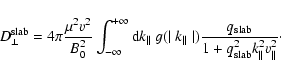
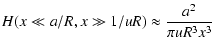
Here we calculate the perpendicular spatial diffusion coefficient
and the corresponding perpendicular mean free path in 2D geometry.
We derive for the perpendicular spatial diffusion coefficient in 2D
turbulence geometry
.
Here we calculate the perpendicular spatial diffusion coefficient
and the corresponding perpendicular mean free path in 2D geometry.
We derive for the perpendicular spatial diffusion coefficient in 2D
turbulence geometry
 |
(83) |
with
 |
(84) |
 |
(85) |
and
 |
(86) |
respectively.
Table 2 shows the approximations for the last two integrals
and for
 ,
yielding approximate formulas for
,
yielding approximate formulas for
 .
With these the perpendicular mean free path of 2D geometry can be
written as
.
With these the perpendicular mean free path of 2D geometry can be
written as
 |
(87) |
If we consider the case
we have
.
Table 2 then implies
 ,
but,
as shown in Sect. 2.8,
in this formal limit the perpendicular cosmic ray transport is no
longer diffusive.
,
but,
as shown in Sect. 2.8,
in this formal limit the perpendicular cosmic ray transport is no
longer diffusive.
For the case of composite geometry we can use Eqs. (80) and (83) to find
with the total fluctuating magnetic field strength
 .
Although not necessary, mainly for illustrating our results we adopt
the same value for
the parameter
.
Although not necessary, mainly for illustrating our results we adopt
the same value for
the parameter
 for the slab and the 2D contribution.
Here we calculate
and
for electrons
and protons
for one set of typical heliospheric parameters and compare them with
the analytical
parallel diffusion results of SS03. For our calculations we use the
same set of
parameters appropriate for interplanetary conditions at 1 AU as Bieber
et al. (1994).
For the magnetic background field we assume
B0=4.12 nT and for
the Alfvén speed
for the slab and the 2D contribution.
Here we calculate
and
for electrons
and protons
for one set of typical heliospheric parameters and compare them with
the analytical
parallel diffusion results of SS03. For our calculations we use the
same set of
parameters appropriate for interplanetary conditions at 1 AU as Bieber
et al. (1994).
For the magnetic background field we assume
B0=4.12 nT and for
the Alfvén speed
 .
For the both parameters
of the
power spectrum we used
.
For the both parameters
of the
power spectrum we used
 and s=5/3.
The parameter
and s=5/3.
The parameter  is assumed to be 1.
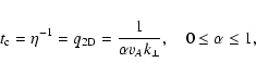
In the following discussions we restrict the rigidity values to the
interesting range
 .
With typical heliospheric parameters we then
always
have
.
With typical heliospheric parameters we then
always
have
 .
.
The value of the spatial diffusion coefficient is given in terms of the
constant
 .
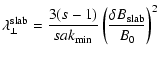
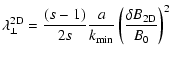
For slab turbulence we
then obtain
.
For slab turbulence we
then obtain
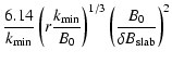
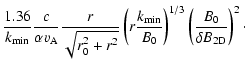
For the 2D coefficient we use Table 2 to obtain
different approximations for
.
In the case
we find from Table 2:
 |
(90) |
and therefore for the perpendicular spatial diffusion coefficient
 |
(91) |
Using heliospheric parameters we obtain
The perpendicular spatial diffusion coefficient for protons and
electrons from slab and 2D turbulence are
shown in Fig. 1.
![\begin{figure}
\par\includegraphics[width=8.6cm,clip]{0470fig1.eps}
\end{figure}](/articles/aa/full/2004/24/aa0470/Timg347.gif) |
Figure 1:
Perpendicular spatial diffusion coefficient of 2D geometry
(solid line) and slab geometry (dotted line) for protons (p+) and
electrons (e-)
for
 . . |
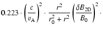
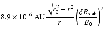
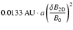
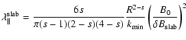
The slab perpendicular mean free path becomes for heliospheric
parameters
where we used that
 m. For the 2D
perpendicular mean free path we obtain under the restriction
:
m. For the 2D
perpendicular mean free path we obtain under the restriction
:
 |
(94) |
which for heliospheric parameters yields
The results for the perpendicular mean free path are shown in Fig. 2.
![\begin{figure}
\par\includegraphics[width=8.7cm,clip]{0470fig2.eps}
\end{figure}](/articles/aa/full/2004/24/aa0470/Timg355.gif) |
Figure 2:
Perpendicular mean free path of 2D geometry (solid line) and
slab geometry (dotted line) for protons (p+) and electrons
(e-)
for
. |
In this subsection we calculate the ratio
for slab, 2D and composite geometry. For
 we
can use the results of SS03
and for
we
can use the results of SS03
and for
 the results of Teufel &
Schlickeiser (2003).
Together with Table 2 we obtain the following results:
the results of Teufel &
Schlickeiser (2003).
Together with Table 2 we obtain the following results:
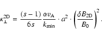
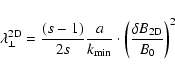
For the case s=5/3 these equations become to
With these results it is simple to calculate the ratio
.
If we do this we obtain for pure slab geometry
 |
(98) |
and for pure 2D geometry
 |
(99) |
These results can be seen in Fig. 3.
![\begin{figure}
\par\includegraphics[width=8.8cm,clip]{0470fig3.eps}
\end{figure}](/articles/aa/full/2004/24/aa0470/Timg370.gif) |
Figure 3:
The ratio
for pure
slab (dotted line)
and pure 2D geometry (solid line) for protons (p+) and electrons
(e-)
for
. |
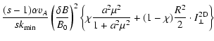
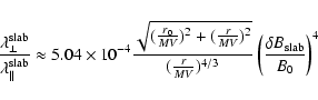
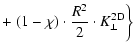
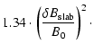
In the case of composite geometry we have
 |
(100) |
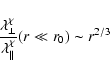
If we assume that  is not too small or too large we find that the
slab component controlls the
parallel mean free path (see SS03)
is not too small or too large we find that the
slab component controlls the
parallel mean free path (see SS03)
 |
(101) |
and the perpendicular mean free path is controlled by the 2D component
 |
(102) |
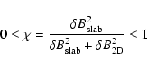
Therefore the ratio of perpendicular and parallel mean free path can be
written as
 |
(103) |
Note the symmetry of the mean free path ratio arround
 due
to the factor
due
to the factor
 in Eq. (103). We find for heliospheric
parameters
in Eq. (103). We find for heliospheric
parameters
 |
|
|
(104) |
Figure 4 shows the results of that ratio for electrons and
Fig. 5 shows the results for protons. In both figures we
calculated the ratio
for
different values of
and for
.
For non-relativistic particles we always find
 |
(105) |
and for relativistic particles
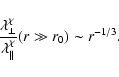 |
(106) |
![\begin{figure}
\par\includegraphics[width=8.8cm,clip]{0470fig4.eps}
\end{figure}](/articles/aa/full/2004/24/aa0470/Timg380.gif) |
Figure 4:
The ratio
as a
function of the rigidity for
electrons for different values of
and for
. |
![\begin{figure}
\par\includegraphics[width=8.8cm,clip]{0470fig5.eps}
\end{figure}](/articles/aa/full/2004/24/aa0470/Timg381.gif) |
Figure 5:
The ratio
as a
function of the rigidity for
protons for different values of
and for
. |
From proton observations we know that (see Palmer 1982)
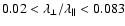 over the rigidity range of
0.5 MV < r < 5 GV. The observations are
not accurate enough to draw conclusions
on the variation of the mean free path ratio with rigidity. By fitting
the appropriate value of
over the rigidity range of
0.5 MV < r < 5 GV. The observations are
not accurate enough to draw conclusions
on the variation of the mean free path ratio with rigidity. By fitting
the appropriate value of
 the observed absolute values are in agreement with the quasilinear
results for all three models: slab, 2D and composite
turbulence. Future more precise observations especially of the rigidity
variation of the ratio of mean free paths
,
both for protons and
electrons, should allow a definite conclusion on the nature of interplanetary
magnetic turbulence from the comparison with our theoretical
predictions contained in Figs. 1-5.
We have presented the quasilinear calculation of perpendicular
diffusion of cosmic ray particles for
weak dynamical magnetic turbulence of arbitrary geometry. Starting from
the equations of motion we went point-by-point through
the derivation of quasilinear
Fokker-Planck coefficients, identifying seven
necessary steps in this derivation. We demonstrated that, in order to have
diffusive behaviour of the
Fokker-Planck coefficients, the existence of a finite
correlation time of the magnetic fluctuations is essential.
the observed absolute values are in agreement with the quasilinear
results for all three models: slab, 2D and composite
turbulence. Future more precise observations especially of the rigidity
variation of the ratio of mean free paths
,
both for protons and
electrons, should allow a definite conclusion on the nature of interplanetary
magnetic turbulence from the comparison with our theoretical
predictions contained in Figs. 1-5.
We have presented the quasilinear calculation of perpendicular
diffusion of cosmic ray particles for
weak dynamical magnetic turbulence of arbitrary geometry. Starting from
the equations of motion we went point-by-point through
the derivation of quasilinear
Fokker-Planck coefficients, identifying seven
necessary steps in this derivation. We demonstrated that, in order to have
diffusive behaviour of the
Fokker-Planck coefficients, the existence of a finite
correlation time of the magnetic fluctuations is essential.
From the perpendicular Fokker-Planck coefficient
we then
deduced the perpendicular spatial
diffusion coefficient
and the associated perpendicular
mean free path
for the damping model of dynamical magnetic turbulence and three
different turbulence geometries: slab, 2D turbulence and composite
turbulence.
For a Kolmogorov-type power spectrum we explicitly
calculated these perpendicular transport parameters for electrons and
protons for realistic heliospheric plasma parameters. The analytical
form of the perpendicular diffusion coefficient is of great interest
for studies of the solar modulation of galactic cosmic rays.
By comparing with our previous determination of the parallel transport
parameters, we are
able to predict the variation of the ratio of mean free paths
with particle rigidity
for the three turbulence models. The comparison of these predictiona
with future accurate experimental determinations of the ratio of mean
free
paths will allow conclusions on the nature of interplanetary magnetic
turbulence.
Acknowledgements
A.S. acknowledges support by the National Science Foundation under
grant ATM-0000315.
R.S. acknowledges support by the Deutsche Forschungsgemeinschaft through
Sonderforschungsbereich 591.
This work was completed while R.S. was a visiting professor at the
University of California
Riverside - Institute of Geophysics and Planetary Physics. R.S. thanks
Gary Zank, Director,
for his kind hospitality and sponsorship through NSF grants ATM-0296113
and ATM-0317509.
-
Bieber, J. W., Matthaeus, W. H., Smith, C. W., et al. 1994, ApJ, 420, 294
NASA ADS
-
Earl, J. A. 1974, ApJ, 193, 231
NASA ADS
-
Giacalone, J., & Jokipii, J. R. 1999, ApJ, 520, 201
-
Gradshteyn, I. S., & Ryzhik, I. M. 1966
(New York: Academic Press)
-
Hall, D. E., & Sturrock, P. A. 1968, Phys. Fluids, 10, 2620
-
Hasselmann, K., & Wibberenz, G. 1968, Z. Geophys., 34, 353
-
Jaekel, U., & Schlickeiser, R. 1992, J. Phys. G: Nucl. Part. Phys., 18,
1089
NASA ADS
-
Le Roux, J. A., Zank, G. P., & Ptuskin, V. S. 1999, JGR, 104, 24845
-
Mace, R. L., Matthaeus, W. H., & Bieber, J. W. 2000, ApJ, 538, 192
NASA ADS
-
Michalek, G. 2001, A&A, 376, 667
NASA ADS
-
Michalek, G., & Ostrowski, M. 1998, A&A, 337, 558
NASA ADS
-
Palmer, I. D. 1982, Rev. Geophys. Space Phys., 20, 2, 335
NASA ADS
-
Schlickeiser, R. 2002 (Berlin: Springer-Verlag)
-
Shalchi, A., & Schlickeiser, R. 2004, ApJ, 604, 861 (SS03)
NASA ADS
-
Teufel, A., & Schlickeiser, R. 2003, A&A, 397, 15
NASA ADS
-
Zank, G. P., Matthaeus, W. H., Bieber, J. W., et al. 1998, JGR, 103, 2085
NASA ADS
7 Online Material
To calculate the Fokker-Planck coefficient in pure 2D geometry we
have to calculate the series
 |
(A.1) |
It is not possible to solve this series analytically without using
approximations. In this paper we use
the same formalism to calculate the series as demonstrated in SS03. To
start our calculations we
write the sum above as
 |
(A.2) |
Now we use the both well known formulas (see Gradshteyn & Ryzhik
1966):
and
to get
| |
|
 |
|
| |
|
 |
(A.5) |
Therefore we obtain
| G(x,y) |
= |
 |
|
| |
|
 |
(A.6) |
Now we can calculate the sum using (Gradshteyn & Ryzhik 1966)
 |
(A.7) |
and we find
Using
 |
(A.9) |
the series G can be finally written as
| G(x,y) |
= |
 |
|
| |
|
 |
(A.10) |
This result is still exact, but to proceed with our calculations we
must consider special cases for
x and y.
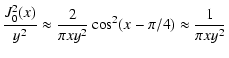
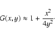
In this case we can consider Eq. (A.10) for small y to obtain
| G(x,y) |
= |
 |
|
| |
= |
 |
(A.11) |
In this case we must develop the functions in Eq. (A.10) up to
the next order:
with these approximations it is simple to calculate G for small
arguments
which can be written as
 |
(A.14) |
In this case Eq. (A.10) can be written as
| G(x,y) |
= |
 |
|
| |
|
![$\displaystyle \times \left[ {\rm e}^{(2 \Theta - \pi) y} + {\rm e}^{-(2 \Theta + \pi) y} \right].$](/articles/aa/full/2004/24/aa0470/img414.gif) |
(A.15) |
With the integral transformation
 we find
| G(x,y) |
= |
 |
|
| |
|
![$\displaystyle \times \left[ {\rm e}^{- z y} + {\rm e}^{-(2 \pi - z) y} \right].$](/articles/aa/full/2004/24/aa0470/img417.gif) |
(A.16) |
Now we consider large y to approximate the integral. If y is a
large number
the contribution to the integral comes from very small values of z
because of the
exponential function. Therefore we can expand the upper limit of the
integral to
infinity and we can approximate the circular functions to obtain:
 |
(A.17) |
The integral is elementary and yields
 |
(A.18) |
We finally find the both cases:
 |
|
|
|
 |
|
|
(A.19) |
Finally all the cases can be written as:
With these approximations it is possible to calculate the perpendicular
Fokker-Planck coefficient for special
cases. We also calculated the series G(x,y) numerically to test Eq.
(A.20). We found that the agreement is accurate for all cases.
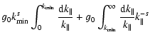
For calculating the Fokker-Planck coefficient in pure 2D geometry we
also
have to calculate the series
 |
(B.1) |
In this section we use the same method to calculate the series as in the
section before. To start our calculations we write the sum above as
 |
(B.2) |
With the well known integral representation for Bessel functions
 |
(B.3) |
we can rewrite the series as
| H(x,y) |
= |
 |
|
| |
|
 |
(B.4) |
Using again Eq. (A.7) we get
H(x,y) =  |
(B.5) |
where we also used
 |
(B.6) |
Now we must consider special cases for x and y to simplify Eq. (B.5).
In this case we can use
 |
(B.7) |
and Eq. (B.6) to find
 |
(B.8) |
If  and
and  we obtain
 |
(B.9) |
In the case of large y Eq. (B.5) can be written as
For deriving this equation we used the same approximations as in
deriving
Eq. (A.17). If we collect all the results we finally find:
With these approximations it is possible to calculate the perpendicular
Fokker-Planck coefficient for special
cases. We also calculated the series H(x,y) numerically to test Eq.
(B.11).
We found that the agreement is accurate for all cases.
In this section we discuss the results for a power spectrum
with finite wave power at small wavenumbers. To do this we
consider
pure
slab- and pure 2D-geometry for the damping model of dynamical magnetic
turbulence:
According to Eq. (46) the Fokker-Planck coefficient can be
written as
 |
(C.1) |
Now we assume a power spectrum with finite wave power at small
wavenumbers:
 |
|
|
(C.2) |
to obtain
and we find
 |
(C.4) |
Note: this is a feature of the damping model of dynamical magnetic
turbulence. If we consider the case of
,
often refered as magnetostatic limit (see
Bieber et al. 1994) we must go
back to Eq. (40):
 |
(C.5) |
Now we use
 |
(C.6) |
and therefore
 |
(C.7) |
to obtain
With this result we can calculate the perpendicular mean free path and
we find
 |
(C.9) |
which is similar to the results derived by Le Roux et al. (1999) and
Zank et al. (1998).
The 2D-Fokker-Planck coefficient can be written as (see Eq. (51))
 |
(C.10) |
with
if we assume a vanishing magnetic helicity. Now we restrict our analysis
to the n=0 contribution
and we find
 |
(C.12) |
and therefore
 |
(C.13) |
if we use the damping model of dynamical magnetic turbulence and the
same power spectrum as in
Eq. (C.2) but now for .
Note: for slab- and for
2D-geometry the
perpendicular Fokker-Planck coefficient goes to infinity if we assume a
power spectrum
with finite wave power at small wavenumbers.
Copyright ESO 2004
![\begin{figure}
\par\includegraphics[width=8.6cm,clip]{0470fig1.eps}
\end{figure}](/articles/aa/full/2004/24/aa0470/img347.gif)
![\begin{figure}
\par\includegraphics[width=8.7cm,clip]{0470fig2.eps}
\end{figure}](/articles/aa/full/2004/24/aa0470/img355.gif)
![\begin{figure}
\par\includegraphics[width=8.8cm,clip]{0470fig3.eps}
\end{figure}](/articles/aa/full/2004/24/aa0470/img370.gif)
![$\displaystyle {1 \over 2} \int_{-1}^{+1} {\rm d} \mu
\left[D_{XX}(\mu ) + D_{YY}(\mu )\right]$](/articles/aa/full/2004/24/aa0470/img30.gif)
![$\displaystyle {\mu v \over \sqrt{2} B_0}\sum_{n=-\infty}^\infty
\int {\rm d}^3k\; \left[ \delta b_R(\vec{k},t)+\delta b_R(\vec{k},t) \right]$](/articles/aa/full/2004/24/aa0470/img54.gif)
![$\displaystyle \qquad\times
\left. (J_{n+1}(W){\rm e}^{\imath \psi }+J_{n-1}(W){\rm e}^{-\imath \psi } \right]
\bigg\}\cdot$](/articles/aa/full/2004/24/aa0470/img108.gif)

![$\displaystyle + \left. \int_{t{'}}^t{\rm d}t{''}\; {\rm e}^{\imath \beta _n\left(t{'}-t{''}\right)-\eta
\left(t{''}-t{'}\right)}\right].$](/articles/aa/full/2004/24/aa0470/img133.gif)
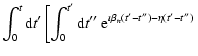
![$\displaystyle \int_0^t{\rm d}t{'}\left[\int_0^{t{'}}{\rm d}s_1\;
{\rm e}^{-(\et...
...\left. \int_0^{t-t{'}}{\rm d}s_2\; {\rm e}^{-(\eta +\imath \beta
_n)s_2}\right]$](/articles/aa/full/2004/24/aa0470/img134.gif)
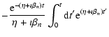
![$\displaystyle \int_0^t{\rm d}t{'}\left[{1-{\rm e}^{-(\eta -\imath \beta _n)t{'}...
... +\imath \beta _n\right)\left(t-t{'}\right)}\over \eta +\imath \beta _n}\right]$](/articles/aa/full/2004/24/aa0470/img135.gif)
![$\displaystyle {1\over \eta -\imath \beta _n}\left[t-{1-{\rm e}^{-\left(\eta -\i...
...a_n\right)t}\over \eta -\imath \beta _n}\right]
+{t\over \eta +\imath \beta _n}$](/articles/aa/full/2004/24/aa0470/img136.gif)
![$\displaystyle {2\eta \over \eta ^2+\beta _n^2}\left[t-{2\beta _n{\rm e}^{-\eta t}\sin
\beta _nt\over \eta ^2+\beta _n^2}\right]$](/articles/aa/full/2004/24/aa0470/img139.gif)
![$\displaystyle - {2\left(\eta ^2-\beta _n^2\right)\over \left(\eta ^2+\beta _n^2\right)^2}\left[1-{\rm e}^{-\eta t} \cos \beta _nt\right].$](/articles/aa/full/2004/24/aa0470/img140.gif)
![$\displaystyle + J_{n-1}(W){\rm e}^{-\imath \psi }\big)\big] \bigg\}\cdot$](/articles/aa/full/2004/24/aa0470/img151.gif)
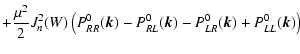
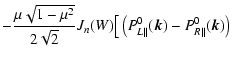
![$\displaystyle - \left. J_{n-1}(W){\rm e}^{-\imath \psi }\right)\big] \bigg\}.$](/articles/aa/full/2004/24/aa0470/img173.gif)


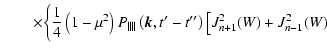
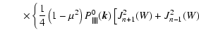
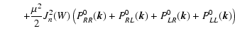
![$\displaystyle + 2 \sigma \mu \sqrt{1 - \mu^2} J_{n}(W) \left( J_{n+1} (W)
- J_{n-1} (W) \right) \bigg].$](/articles/aa/full/2004/24/aa0470/img221.gif)
![$\displaystyle \times \left[ {\left(1-\mu^2\right)\over 2} \left( J_{n+1}^2 (W) + J_{n-1}^2 (W) \right)
+ \mu^2 J_n^2 (W) \right],$](/articles/aa/full/2004/24/aa0470/img229.gif)

![$\displaystyle 1.34 \cdot \left[ 1 -
{\arctan{a} \over a} \right] \left( {\delta B_{\rm slab}\over B_0} \right)^2$](/articles/aa/full/2004/24/aa0470/img340.gif)
![$\displaystyle 0.08~ {\rm AU} \cdot \left[ {1 \over a} -
{\arctan{a}
\over a^2} \right] \left( {\delta B_{\rm slab}\over B_0} \right)^2$](/articles/aa/full/2004/24/aa0470/img348.gif)

![\begin{figure}
\par\includegraphics[width=8.8cm,clip]{0470fig4.eps}
\end{figure}](/articles/aa/full/2004/24/aa0470/img380.gif)
![\begin{figure}
\par\includegraphics[width=8.8cm,clip]{0470fig5.eps}
\end{figure}](/articles/aa/full/2004/24/aa0470/img381.gif)

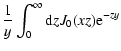
![$\displaystyle {1 \over y} \int_0^{\pi} {\rm d} z J_0 \left(2 x \sin \left( {z
\...
...2} \right) \right) \cdot \left[ {\rm e}^{-zy} + {\rm e}^{-(2 \pi - z)y} \right]$](/articles/aa/full/2004/24/aa0470/img442.gif)