![\begin{figure}
\par\resizebox{8.8cm}{!}{\includegraphics[clip]{H4473F1.eps}}
\end{figure}](/articles/aa/full/2004/07/aah4473/img16.gif) |
Figure 1: Optical image of the pair NGC 3718 (to the west) and NGC 3729 (to the east). Taken from the DSS service. |
| Open with DEXTER | |
In the text
![\begin{figure}
\par\resizebox{8.8cm}{!}{\includegraphics[clip]{H4473F2corr.eps}}
\end{figure}](/articles/aa/full/2004/07/aah4473/img17.gif) |
Figure 2: Optical image of NGC 3718. Taken from the DSS survey. |
| Open with DEXTER | |
In the text
![\begin{figure}
\par\resizebox{8.8cm}{!}{\begin{turn}{-90}\includegraphics[clip]{H4473F3.eps}\end{turn}}
\end{figure}](/articles/aa/full/2004/07/aah4473/img46.gif) |
Figure 3: A map of the pointing coordinates, observed at the two observing runs. The respective observed frequencies are marked as: black diamonds (CO(1-0)), red crosses (CO(2-1)) and blue squares (HCN(1-0)). |
| Open with DEXTER | |
In the text
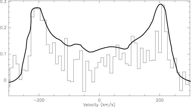 |
Figure 4:
Global CO(1-0) spectrum, obtained by summing
up all individual spectra, measured at the positions given in
Fig. 3. The intensity scale is in units of
|
| Open with DEXTER | |
In the text
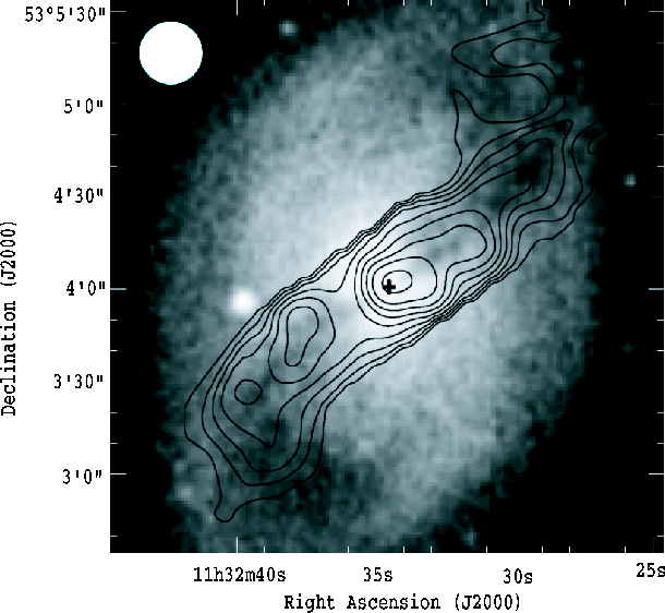 |
Figure 5:
Integrated line intensity map of
CO(1-0) with linear contour lines (steps:
|
| Open with DEXTER | |
In the text
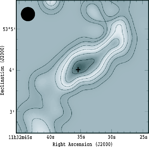 |
Figure 6:
Integrated intensity map of CO(2-1). The
contours correspond to 0.2, 0.4, 0.6 times K km s-1. The cross
indicates the optical center. The map is convolved to the 21
|
| Open with DEXTER | |
In the text
![\begin{figure}
\par\resizebox{8.8cm}{!}{\begin{turn}{0}\includegraphics[clip]{H4473F7corr.eps}\end{turn}}
\end{figure}](/articles/aa/full/2004/07/aah4473/img54.gif) |
Figure 7:
The position-velocity-diagram of NGC 3718,
obtained in
|
| Open with DEXTER | |
In the text
![\begin{figure}
\par\resizebox{8.8cm}{!}{\begin{turn}{-90}\includegraphics[clip]{H4473F8.eps}\end{turn}}
\end{figure}](/articles/aa/full/2004/07/aah4473/img80.gif) |
Figure 8:
The CO(1-0) spectrum in the center. Vertical
scale is
|
| Open with DEXTER | |
In the text
![\begin{figure}
\par\resizebox{8.8cm}{!}{\begin{turn}{-90}\includegraphics[clip]{H4473F9.eps}\end{turn}}
\end{figure}](/articles/aa/full/2004/07/aah4473/img81.gif) |
Figure 9:
The CO(2-1) spectrum in the center. Vertical
scale is
|
| Open with DEXTER | |
In the text
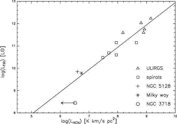 |
Figure 10:
NGC 3718 has the same ratio of FIR to HCN
luminosity as ULIRGs (black triangles) and normal spirals (red squares).
NGC 5128 (blue asterisk) and the Milky Way (green cross) are
shown for comparison as well. The blue circle shows the upper limit of
|
| Open with DEXTER | |
In the text
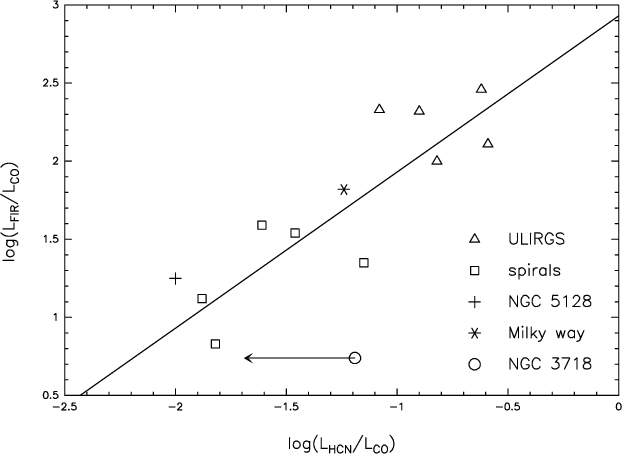 |
Figure 11: Comparison of the fraction of dense gas to the star formation efficiency (Solomon et al. 1992). Symbols are the same as in Fig. 10. |
| Open with DEXTER | |
In the text
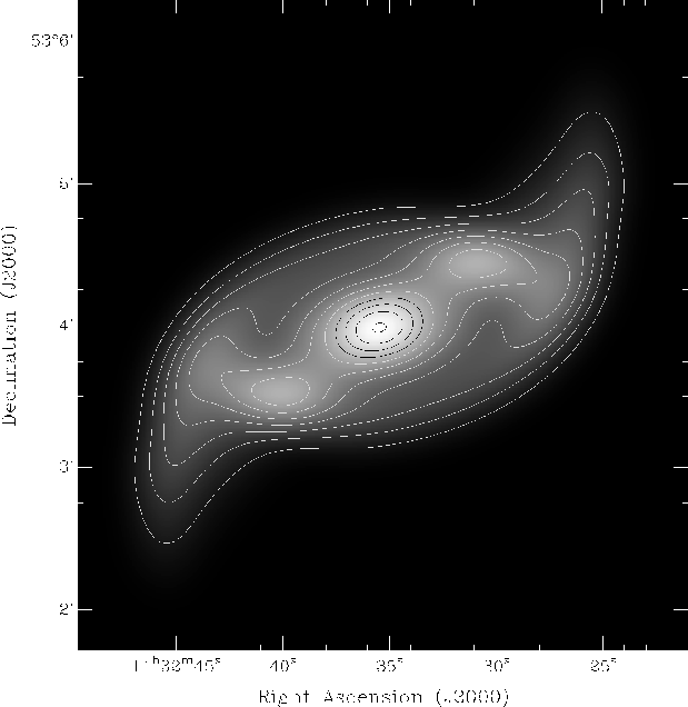 |
Figure 12: The modeled integrated CO(1-0) line intensity shown with linear-scale contours. |
| Open with DEXTER | |
In the text
![\begin{figure}
\par\resizebox{8.8cm}{!}{\includegraphics[clip]{H4473F13.eps}}
\end{figure}](/articles/aa/full/2004/07/aah4473/img114.gif) |
Figure 13:
The upper panel shows the rotation curve v(r) used
to model NGC 3718, in the lower panel the corresponding tilting-angles |
| Open with DEXTER | |
In the text
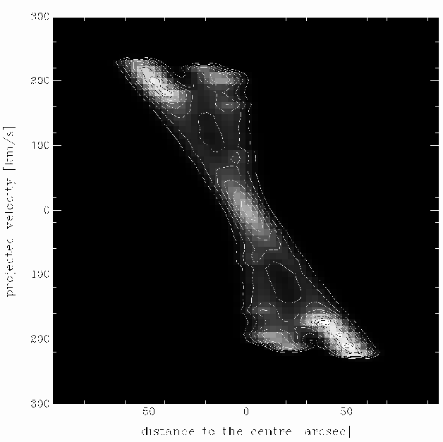 |
Figure 14: The modeled pv-diagram along the major axis of the integrated line-intensity. A linear contour-scale is shown. |
| Open with DEXTER | |
In the text
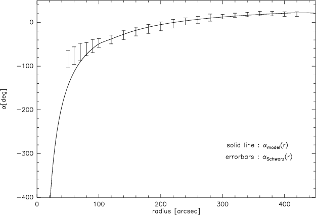 |
Figure 15: The plot shows the curve of nodes of our model (solid line), discussed in Sect. 4. In our model the warp starts at 20'', as one can see in Fig. 13. Furthermore the errorbars are indicating the corresponding values of the HI-rings (Schwarz 1985) in the same frame of reference. |
| Open with DEXTER | |
In the text