R. W. Hanuschik
European Southern Observatory, Karl-Schwarzschild-Str. 2, 85748 Garching, Germany
Received 18 April 2003 / Accepted 19 May 2003
Abstract
This paper presents a flux-calibrated, high-resolution, high-SNR atlas
of optical and near-IR sky emission. It provides a complete template
of the high-resolution night-sky emission spectrum with the deepest
exposures ever obtained from the ground.
The data have been acquired
by UVES, ESO's echelle spectrograph at the 8.2-m UT2 telescope of the Very
Large Telescope (VLT).
Raw data stacks with up to 16 hours of integration time have been combined.
The spectrum covers the range 3140-10 430 Å at a resolving power
of about 45 000. A total of 2810 sky emission lines have been
measured. This high-resolution spectrum is intended to be used
for the identification of previously unknown faint sky lines,
for simulations of ground based observations where the sky background is
important, as a template for checks on the accuracy and stability of
the wavelength scale, and as a reference for the reduction of spectra of
faint objects.
Key words: line: identification - atomic data - atmospheric effects - atlases - techniques: spectroscopic
It has been realized however that there are also positive aspects to the night-sky emission lines, namely that they provide a template for wavelength self-calibration of the science data (e.g. Osterbrock et al. 1996, 1997).
This paper presents a flux-calibrated night-sky emission atlas at high resolution and high SNR. It extends the existing ISAAC infrared atlas (Rousselot et al. 2000; Lidman et al. 2000) towards the optical range and towards higher spectral resolution.
| Setting* | Range (Å) | Number of spectra | Airmass | Seeing | Fractional lunar | Total exposure |
| (month/year) | illumination | time (h) | ||||
|
346 DI1 |
3140-3760 | 7 (06/2001) + | 1.024-1.336 | 0.45-1.09 | 0.002-0.048 | 16.0 |
| 9 (08/2001) | (mean: 1.143) | (mean: 0.68) | (mean: 0.018) | |||
| 437 DI2 |
3740-4860 | 9 (06/2001) + | 1.021-2.047 | 0.39-0.76 | 0.000-0.050 | 13.2 |
| 3 (07/2001) | (mean: 1.241) | (mean: 0.55) | (mean: 0.023) | |||
| 580 DI1 |
L: 4810-5770, | 7 (06/2001) | 1.024-1.321 | 0.62-0.83 | 0.002-0.035 | 7.0 |
| U: 5830-6790 | (mean: 1.144) | (mean: 0.72) | (mean: 0.014) | |||
| 860 DI2 |
L: 6700-8560, | 9 (06/2001) | 1.021-1.412 | 0.40 .. 0.57 | 0.000-0.050 | 9.0 |
| U: 8600-10 430 | (mean: 1.108) | (mean: 0.50) | (mean: 0.025) |
* Central wavelength in nm, dichroic filter,
binning; L = lower red CCD, U = upper red CCD.
![\begin{figure}
\par\includegraphics[width=17.75cm,clip]{extract.ps}\end{figure}](/articles/aa/full/2003/33/aa3874/img7.gif) |
Figure 2: 2D extracted (bottom) and 1D extracted spectrum (top). The central order marked in Fig. 1 has been selected here. Wavelength scale increases towards the right. The two sky windows are marked. The collapsed 1D sky spectrum has been constructed from these two windows. The features accepted and measured as sky emission lines are marked by open triangles. |
Input data have been obtained with ESO's echelle spectrograph UVES (Dekker et al. 2000) mounted at the 8.2-m UT2 (Kueyen) telescope of the VLT array on Paranal. The aim of the atlas is to accurately determine night-sky emission line positions and fluxes. These data are potentially useful for deep spectroscopy of point and extended sources, but also for other applications, e.g. aeronomy. The advantages of the present atlas over the existing data from the Keck 10 m telescope (Osterbrock et al. 1996, 1997) are the flux calibration, the higher number of line positions, the higher SNR and the extension to the blue. It also provides a useful supplement of the recent UBVRI Paranal night sky survey of Patat (2003).
For the same reason it has been very important to find well-centred spectra from point-like sources. Input frames were visually checked for proper centring and against contamination by multiple sources or extended background emission.
The slit width in all spectra was 1.0
![]() .
This is a reasonable trade-off between highest SNR
and highest spectral resolution. The slit width of 1.0
.
This is a reasonable trade-off between highest SNR
and highest spectral resolution. The slit width of 1.0
![]() translates into resolving power
R = 45 000 in the blue, and
43 000 in the red. Selected input data are summarized in Table
1.
translates into resolving power
R = 45 000 in the blue, and
43 000 in the red. Selected input data are summarized in Table
1.
All spectra have been obtained in Service Mode runs. Most data were collected around the new moon of June 2001 (nights 20-22/06/2001). Some spectra have been added from the new moon periods of July 2001 (nights 18-21/07/2001) and August 2001 (nights 16-19/08/2001).
UVES has a mosaic of one blue and two red CCDs.
Two blue standard settings were selected (central wavelength
346 nm, dichroic filter #1 and 437 nm, dichroic #2), and two red standard settings (580 nm, dichroic #1, and 860 nm,
dichroic #2), all in binned mode (![]() ).
The data cover the whole wavelength range accessible to UVES.
).
The data cover the whole wavelength range accessible to UVES.
The spectra have been reduced with the UVES pipeline (version 1.7.0) (Ballester et al. 2000), using pipeline-processed master calibration data from the same period. Two steps were necessary:
1. All spectra per setting and per period were stacked and combined, in order to remove cosmic ray hits and improve the SNR (see Fig. 1). This step made use of the uves_cal_mkmaster recipe which is usually employed to stack sets of raw BIAS or FLAT data. Cosmic ray removal was very efficient.
2. The stacked science data were then reduced with the standard recipe for science reduction, uves_obs_scired. Extraction mode was "2D'', which means the data were de-biased, flattened, wavelength-calibrated, merged, and resampled to a two-dimensional wavelength-Y grid where Y is the vertical slit coordinate (Fig. 2).
The blue data come from two different epochs (Table 1), with two different grating orientations. They were co-added per period and reduced separately. Only after full reduction were the results averaged into the final result. All data from within the same period (covering a few days) were reduced with the same wavelength calibration and flat field files.
In the blue, two sky windows of 4 binned pixels each (2
![]() )
were finally
extracted, located at the upper and lower
boundaries (SKY1 and SKY2, see Fig. 2),
thereby avoiding contamination from the signal source. The width of the sky windows was chosen
empirically. Figure 3 shows cross-dispersion profiles for the bluest data. The final 1D sky spectrum was
obtained from collapsing and averaging the two sky windows.
)
were finally
extracted, located at the upper and lower
boundaries (SKY1 and SKY2, see Fig. 2),
thereby avoiding contamination from the signal source. The width of the sky windows was chosen
empirically. Figure 3 shows cross-dispersion profiles for the bluest data. The final 1D sky spectrum was
obtained from collapsing and averaging the two sky windows.
In the red, a regular pipeline-provided 1D extraction of the science spectrum delivered extracted and averaged sky windows as a by-product. This product was chosen as 1D spectrum since it has a better merging algorithm for the echelle orders.
Both the extracted (1D) and rectified but otherwise unextracted (2D) results was used for the following line measurements because both have their specific pros and cons. The 2D spectra are superior for line measurements and reliability assessment. The pipeline-delivered results have however their limitations, e.g. flat-field artefacts, a crude order merging algorithm and a narrower wavelength coverage. The 1D spectra (obtained from averaging the 2D data in the blue, and from direct pipeline extraction of the input data in the red) provide better emission line plots and higher SNR but limited capacity for recognizing noise and artefacts.
The extracted spectra still carry some large-scale signature of the spectrograph, namely the ratio of sky emission and
flat field spectral slopes. To obtain calibrated fluxes,
master response curves were used. These were
derived from a large set of flux standard star measurements obtained over roughly the same period as the input
spectra![]() .
.
A typical UVES night sees standard star measurements with a 10
![]() slit in the evening and in the morning
twilight. The UVES pipeline creates from each input standard star frame a response curve by dividing the extracted
signal into the tabulated physical flux of the standard star. These response curves need to be corrected for exposure
time, binning, gain and extinction. Furthermore they show stellar spectral features which need to be treated properly
before they are compared to the tabulated flux values. These values typically
come on a 50 Å grid.
slit in the evening and in the morning
twilight. The UVES pipeline creates from each input standard star frame a response curve by dividing the extracted
signal into the tabulated physical flux of the standard star. These response curves need to be corrected for exposure
time, binning, gain and extinction. Furthermore they show stellar spectral features which need to be treated properly
before they are compared to the tabulated flux values. These values typically
come on a 50 Å grid.
It is also obvious that the quality of the nights, and of the standard star fluxes, vary. It is therefore necessary to carefully select night-by-night response curves. The results of the correction and selection steps are called the master response curves. These provide a high-quality flux calibration of the relative slope of the spectrum. The absolute scale of the flux-calibrated spectrum may still suffer from systematic effects like slit losses and variability of the photometric quality in a night.
For the flux calibration of the UVES sky spectrum, a set of master response curves was selected which is valid for the period 01/06/2001 until 30/09/2001 (Fig. 4).
The following expression has been used for the flux calibration of the sky emission spectra:
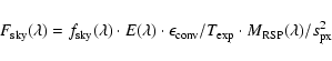 |
(1) |
The flux calibration of the sky emission spectra has some specific problems:
Extinction correction. The major part of the sky emission spectrum is due to OH Meinel bands and arises in
atmospheric heights of typically 90 km (Leinert et al. 1998). Light emitted at those altitudes can be expected to suffer from
essentially the same extinction as light from extraterrestrial sources.
However, the emission layer of finite distance and extent introduces a
special geometric effect. The optical path length through a layer of
thickness l0 along a line of sight
at airmass X increases with X,
![]() (Roach & Meinel
1955; Garstang 1989). This causes the night sky emission to
brighten towards the horizon.
(Roach & Meinel
1955; Garstang 1989). This causes the night sky emission to
brighten towards the horizon.
This is applicable, however, for only a fraction f of the continuum sky emission which is of atmospheric origin, while the remaining fraction (1-f) is from diffuse extraterrestrial sources and does not show that effect (Patat 2003).
Assumptions on f are very uncertain. It is also well
known that sky emission is highly variable (see Patat 2003).
Therefore only a standard
extinction
correction was applied which focuses on the leading effect, namely
the extinction which is strongly chromatic, especially in
the blue:
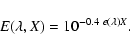 |
(2) |
| Setting* |
|
|
|
| (s-1) | (
|
||
|
346 DI1 |
3600 | 0.60 | 0.246*2 |
| 437 DI2 |
3876 | 0.60 | 0.246*2 |
| 580 DI1 |
3600 | 0.52 | 0.182*2 |
| 860 DI2 |
3600 | 0.52 | 0.182*2 |
* Central wavelength in nm, dichroic filter,
binning.
Neglecting the geometric brightening in principle leads to an overcorrection of extinction, and hence the sky emission flux. Using the UBVRI extinction coefficients for Paranal from Patat's Table A.1, the mean airmass values from Table 1, and f = 0.6 (Patat's Appendix C), the effect of the overshoot can be estimated. The result is that on average the corrected fluxes may be too high by about 0.10 mag (less in the red, more in the 437 setting with its higher average airmass), with no strong wavelength dependence. We will ignore that potential effect in the following.
Contamination. As much care as possible has been taken to select data from really dark time (see Sect. 2).
Also contamination has been avoided as far as possible, either from the seeing wings of the
scientific objects or from extraterrestrial diffuse emission (such as
extended HII regions).
All input raw frames have been inspected
to have seeing better than 1
![]() .
The median stacking process is expected to remove background emission
outliers. Residual contamination, if present at all, is likely to be very small.
.
The median stacking process is expected to remove background emission
outliers. Residual contamination, if present at all, is likely to be very small.
Intrinsic variability. Sky emission lines are well known to be variable on various time and spatial scales. The input data used here have been collected from different nights and from long exposures. The measured line fluxes are therefore an average only.
Setting 346_DI1_
![]() . The master response curve for this setting is established redwards of 3300 Å only, because of
the standard stars used during the validity period. The curve used here has been extrapolated bluewards towards
3100 Å using a second-order polynomial.
. The master response curve for this setting is established redwards of 3300 Å only, because of
the standard stars used during the validity period. The curve used here has been extrapolated bluewards towards
3100 Å using a second-order polynomial.
Setting 437_DI2_
![]() . The flux calibration in this setting might be less certain than in the other settings because of
the intrinsic uncertainties of the master response curve in the Balmer jump region.
. The flux calibration in this setting might be less certain than in the other settings because of
the intrinsic uncertainties of the master response curve in the Balmer jump region.
The flux-calibrated UVES sky emission spectrum has been collected in two forms:
The bottom part of Fig. 5 shows the flux-calibrated night-sky spectrum, sampled to 5 Å to illustrate the continuum slope. Steps between certain portions of the spectrum presumably come from uncertainties in the extraction of the faint sky continuum flux. The full spectrum is plotted in Figs. 7-41.
Before discussing the sky emission spectrum in more depth, we want to focus on measurements of the emission lines, in order to disentangle continuum and line emission.
Apart from providing the flux-calibrated sky emission spectrum, the second purpose of this paper is to derive accurate emission line positions and strengths. For that purpose the 2D spectra, the extracted SKY1 and SKY2 spectra, and their error (expressed as rms of the difference spectra) have been used. We aim to provide input data for spectroscopic identifications. A starting point for these may be found e.g. in Osterbrock et al. (1996, 1997), in Abrams et al. (1994), and in Rousselot et al. (2000).
It turned out that the main challenge is not to find emission lines but to reject false lines due to e.g. reduction or CCD artefacts, residual cosmic rays or just noise. The following criteria had to be met for a line to be accepted for the catalogue:
The list of measured lines can be claimed as being almost complete at the resolution and SNR level of the input data. Those spectral regions corresponding to the beginning of a new echelle order may still hide some features in enhanced noise. There are also small spectral gaps of a few Å between the redmost orders beyond 9760 Å (see Figs. 36-38), and two larger gaps of about 40-60 Å at the central wavelengths of the two red settings (5800 and 8600 Å) due to the physical gaps between the two red CCDs in the mosaic.
Once a feature had been assessed as a valid emission line, a Gaussian fitting routine was employed to obtain the central wavelength, the central flux, and the FWHM of the fit. These three parameters (called CENTER, FLUX, and FWHM) are listed in the result tables, together with the line intensity from uncalibrated spectra (INT).
| Setting* | Range (Å) | Typical level | Number of | Average contribution |
| of sky continuum1 | sky emission lines | from sky emission lines2 | ||
|
346 DI1 |
3140-3760 | 0.17 | 373 | 0.02 |
| 437 DI2 |
3740-4860 | 0.14 | 565 | 0.01 |
| 580 DI1 |
L: 4800-5770 | 0.09 | 88 | 0.02 |
| 580 DI1 |
U: 5830-6790 | 0.10 | 172 | 0.04 |
| 860 DI2 |
L: 6700-8560 | 0.08 | 1014 | 0.01 |
| 860 DI2 |
U: 8600-10 430 | 0.07 | 589 | 0.40 |
|
* Central wavelength in nm, dichroic filter, binning;
L: lower red CCD, U: upper red CCD. 1 In 2 Averaged across 50 Å, same units as above. |
Line blends that would be considered as resolved with a simple cursor-marked approach are still a blend for the Gaussian fit procedure unless two peaks are clearly separated. Hence some of the lines catalogued here are indeed marginally resolved blends with a FWHM in excess of the resolution limit.
The internal accuracy of the wavelength scale is measured by the rms of the difference between
the global dispersion solution and the arclamp emission lines.
The mean rms values for binned data range
between 4.7 mÅ for the 346 nm setting and 10 mÅ for the 860 nm
setting![]() . These numbers translate into 1/15-1/20 resolution elements.
. These numbers translate into 1/15-1/20 resolution elements.
The FWHM values of the measured lines cluster very closely around the nominal values expected from the resolving power. This means that the process of averaging the data from several days, and from different epochs in the case of the blue data, has not introduced systematic shifts degrading the spectral resolution.
A simple cross-check of the precision of the line positions is the
comparison between the line positions as listed in the Keck atlas and in
the present atlas. The difference
| (3) |
| (4) |
Figures 7-41, published electronically, show the extracted UVES sky emission spectrum. Tables 4-9, available at the CDS, list the positions, widths and fluxes for all sky emission lines.
The spectrum is plotted in 20 or 30 Å panels, with starting and end wavelength denoted at the borders. The figures are arranged as follows:
The plots redward of 6000 Å have markings for the
positions of
identified OH lines in the Rousselot et al. (2000) list.
Line positions below 9975 Å have been taken
from the extended list (Lidman et al. 2000).
All positions have been transformed from vacuum to
air using the Edlén (1966) formula:
| |
= | ||
| n | = | 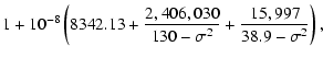 |
(5) |
The top part of Fig. 5 shows the total sky emission flux averaged over 50 Å, and the continuum flux separately.
Below 5500 Å, sky emission lines generally do not contribute significantly to the total sky emission flux. Although
locally emission lines are frequent, they are all faint. Between 5500 Å and 6500 Å, the strong atomic sky emission
lines of [O I] (
![]() 5577.35, 6300.30, and 6363.78 Å) add significant flux. Above 6500 Å, line emission quickly gets
stronger. This is due both to the increasing number and
strength of emission lines.
Above 8600 Å the averaged flux from emission lines is a factor of 6 higher than the continuum
emission. These numbers become relevant for measurements with spectrographs with lower resolution.
5577.35, 6300.30, and 6363.78 Å) add significant flux. Above 6500 Å, line emission quickly gets
stronger. This is due both to the increasing number and
strength of emission lines.
Above 8600 Å the averaged flux from emission lines is a factor of 6 higher than the continuum
emission. These numbers become relevant for measurements with spectrographs with lower resolution.
Even if their average value is negligible in all but the redmost optical spectral ranges, fluxes of sky emission lines become relevant locally. As Table 3 shows, their number may locally be rather high and even, in the near-IR, dominate the whole spectrum.
In total, positions, widths and peak fluxes for N = 2810 emission lines have been measured. The strongest are at 103 times the sky emission continuum. The UV-blue has many resolved lines from the rotational bands of O2, specifically the Herzberg I and Chamberlain bands. Their intensity is up to 10 times the continuum value. They appear all the way down to our spectral limit, about 3140 Å.
The wavelength range 4000-5500 Å is sparsely populated. The red spectra are dominated by OH (Meinel) lines, with some regions with strong telluric O2 absorption.
This paper provides the flux-calibrated optical night-sky emission spectrum for the wavelength range 3140-10 400 Å
measured at high resolution with the echelle spectrograph UVES.
It is based on the deepest high-resolution exposures of the night-sky emission taken so far.
Faint continuum sky emission has a level of
![]() cgs.
A total of 2810 night-sky emission lines
has been carefully selected and measured,
with an average accuracy of 17 mÅ.
cgs.
A total of 2810 night-sky emission lines
has been carefully selected and measured,
with an average accuracy of 17 mÅ.
This set of data could become useful to serve as a template for the subtraction of sky emission lines and for wavelength calibration. The night-sky emission flux can be used as an input for exposure time calculators and for planning sky-limited observations.
Figures 7-41 are published in electronic form![]() .
Tables 4-9, along with the 1D-spectra as FITS files, are available in electronic form
.
Tables 4-9, along with the 1D-spectra as FITS files, are available in electronic form![]() .
There is
also a web site for rapid browsing
.
There is
also a web site for rapid browsing![]() .
.
ESO is interested in collaborations for an ongoing analysis of the data material presented here.
Acknowledgements
RWH would like to thank Jean-Gabriel Cuby from Paranal Science Operations for initiating this project, Sandro D'Odorico for many useful suggestions and Nando Patat for stimulating discussions about extinction correction.
![\begin{figure}
\par\includegraphics[width=15cm,clip]{VERSION_ELEC/3460_1.ps}\end{figure}](/articles/aa/full/2003/33/aa3874/img37.gif) |
Figure 7:
The night-sky spectrum as seen by UVES, covering
the wavelength range
|
![\begin{figure}
\par\includegraphics[width=15cm,clip]{VERSION_ELEC/3460_2.ps}\end{figure}](/articles/aa/full/2003/33/aa3874/img38.gif) |
Figure 8: Same as Fig. 7, for range 3300-3460 Å. |
![\begin{figure}
\par\includegraphics[width=15cm,clip]{VERSION_ELEC/3460_3.ps}\end{figure}](/articles/aa/full/2003/33/aa3874/img39.gif) |
Figure 9: Same as Fig. 7, for range 3460-3620 Å. |
![\begin{figure}
\par\includegraphics[width=15cm,clip]{VERSION_ELEC/3460_4.ps}\end{figure}](/articles/aa/full/2003/33/aa3874/img40.gif) |
Figure 10: Same as Fig. 7, for range 3620-3760 Å. |
![\begin{figure}
\par\includegraphics[width=15cm,clip]{VERSION_ELEC/4370_1.ps}\end{figure}](/articles/aa/full/2003/33/aa3874/img41.gif) |
Figure 11: UVES night-sky spectrum, covering 3740-3900 Å. The vertical bars mark line measurements from this atlas. See the text of the Appendix for more general information about these plots. |
![\begin{figure}
\par\includegraphics[width=15cm,clip]{VERSION_ELEC/4370_2.ps}\end{figure}](/articles/aa/full/2003/33/aa3874/img42.gif) |
Figure 12: Same as Fig. 11, for range 3900-4060 Å. |
![\begin{figure}
\par\includegraphics[width=15cm,clip]{VERSION_ELEC/4370_3.ps}\end{figure}](/articles/aa/full/2003/33/aa3874/img43.gif) |
Figure 13: Same as Fig. 11, for range 4060-4220 Å. |
![\begin{figure}
\par\includegraphics[width=15cm,clip]{VERSION_ELEC/4370_4.ps}\end{figure}](/articles/aa/full/2003/33/aa3874/img44.gif) |
Figure 14: Same as Fig. 11, for range 4220-4380 Å. |
![\begin{figure}
\par\includegraphics[width=15cm,clip]{VERSION_ELEC/4370_5.ps}\end{figure}](/articles/aa/full/2003/33/aa3874/img45.gif) |
Figure 15: Same as Fig. 11, for range 4380-4540 Å. |
![\begin{figure}
\par\includegraphics[width=15cm,clip]{VERSION_ELEC/4370_6.ps}\end{figure}](/articles/aa/full/2003/33/aa3874/img46.gif) |
Figure 16: Same as Fig. 11, for range 4540-4700 Å. |
![\begin{figure}
\par\includegraphics[width=15cm,clip]{VERSION_ELEC/4370_7.ps}\end{figure}](/articles/aa/full/2003/33/aa3874/img47.gif) |
Figure 17: Same as Fig. 11, for range 4700-4860 Å. |
![\begin{figure}
\par\includegraphics[width=15cm,clip]{VERSION_ELEC/5800L_2.ps}\end{figure}](/articles/aa/full/2003/33/aa3874/img49.gif) |
Figure 19: Same as Fig. 18, for range 5050-5290 Å. |
![\begin{figure}
\par\includegraphics[width=15cm,clip]{VERSION_ELEC/5800L_3.ps}\end{figure}](/articles/aa/full/2003/33/aa3874/img50.gif) |
Figure 20: Same as Fig. 18, for range 5290-5530 Å. |
![\begin{figure}
\par\includegraphics[width=15cm,clip]{VERSION_ELEC/5800L_4.ps}\end{figure}](/articles/aa/full/2003/33/aa3874/img51.gif) |
Figure 21: Same as Fig. 18, for range 5530-5770 Å. |
![\begin{figure}
\par\includegraphics[width=14.7cm,clip]{VERSION_ELEC/5800U_2.ps}\end{figure}](/articles/aa/full/2003/33/aa3874/img53.gif) |
Figure 23: Same as Fig. 22, for range 6070-6310 Å. |
![\begin{figure}
\par\includegraphics[width=15cm,clip]{VERSION_ELEC/5800U_3.ps}\end{figure}](/articles/aa/full/2003/33/aa3874/img54.gif) |
Figure 24: Same as Fig. 22, for range 6310-6550 Å. |
![\begin{figure}
\par\includegraphics[width=15cm,clip]{VERSION_ELEC/5800U_4.ps}\end{figure}](/articles/aa/full/2003/33/aa3874/img55.gif) |
Figure 25: Same as Fig. 22, for range 6550-6790 Å. |
![\begin{figure}
\par\includegraphics[width=15cm,clip]{VERSION_ELEC/8600L_2.ps}\end{figure}](/articles/aa/full/2003/33/aa3874/img57.gif) |
Figure 27: Same as Fig. 26, for range 6940-7180 Å. |
![\begin{figure}
\par\includegraphics[width=15cm,clip]{VERSION_ELEC/8600L_3.ps}\end{figure}](/articles/aa/full/2003/33/aa3874/img58.gif) |
Figure 28: Same as Fig. 26, for range 7180-7420 Å. |
![\begin{figure}
\par\includegraphics[width=15cm,clip]{VERSION_ELEC/8600L_4.ps}\end{figure}](/articles/aa/full/2003/33/aa3874/img59.gif) |
Figure 29: Same as Fig. 26, for range 7420-7660 Å. |
![\begin{figure}
\par\includegraphics[width=15cm,clip]{VERSION_ELEC/8600L_5.ps}\end{figure}](/articles/aa/full/2003/33/aa3874/img60.gif) |
Figure 30: Same as Fig. 26, for range 7660-7900 Å. |
![\begin{figure}
\par\includegraphics[width=15cm,clip]{VERSION_ELEC/8600L_6.ps}\end{figure}](/articles/aa/full/2003/33/aa3874/img61.gif) |
Figure 31: Same as Fig. 26, for range 7900-8140 Å. |
![\begin{figure}
\par\includegraphics[width=15cm,clip]{VERSION_ELEC/8600L_7.ps}\end{figure}](/articles/aa/full/2003/33/aa3874/img62.gif) |
Figure 32: Same as Fig. 26, for range 8140-8380 Å. |
![\begin{figure}
\par\includegraphics[width=15cm,clip]{VERSION_ELEC/8600L_8.ps}\end{figure}](/articles/aa/full/2003/33/aa3874/img63.gif) |
Figure 33: Same as Fig. 26, for range 8380-8560 Å. |
![\begin{figure}
\par\includegraphics[width=14.7cm,clip]{VERSION_ELEC/8600U_2.ps}\end{figure}](/articles/aa/full/2003/33/aa3874/img65.gif) |
Figure 35: Same as Fig. 34, for range 8840-9080 Å. |
![\begin{figure}
\par\includegraphics[width=15cm,clip]{VERSION_ELEC/8600U_3.ps}\end{figure}](/articles/aa/full/2003/33/aa3874/img66.gif) |
Figure 36: Same as Fig. 34, for range 9080-9320 Å. |
![\begin{figure}
\par\includegraphics[width=15cm,clip]{VERSION_ELEC/8600U_4.ps}\end{figure}](/articles/aa/full/2003/33/aa3874/img67.gif) |
Figure 37: Same as Fig. 34, for range 9320-9560 Å. |
![\begin{figure}
\par\includegraphics[width=15cm,clip]{VERSION_ELEC/8600U_5.ps}\end{figure}](/articles/aa/full/2003/33/aa3874/img68.gif) |
Figure 38: Same as Fig. 34, for range 9560-9800 Å. There is a small gap near 9765 Å, due to incomplete spectral coverage by the CCD. |
![\begin{figure}
\par\includegraphics[width=15cm,clip]{VERSION_ELEC/8600U_6.ps}\end{figure}](/articles/aa/full/2003/33/aa3874/img69.gif) |
Figure 39: Same as Fig. 34, for range 9800-10 040 Å. There is a small gap near 9922 Å, due to incomplete spectral coverage by the CCD. |
![\begin{figure}
\par\includegraphics[width=15cm,clip]{VERSION_ELEC/8600U_7.ps}\end{figure}](/articles/aa/full/2003/33/aa3874/img70.gif) |
Figure 40: Same as Fig. 34, for range 10 040-10 280 Å. There are two gaps near 10086 Å and 10253 Å due to incomplete spectral coverage by the CCD. |
![\begin{figure}
\par\includegraphics[width=16cm,clip]{VERSION_ELEC/8600U_8.ps}\end{figure}](/articles/aa/full/2003/33/aa3874/img71.gif) |
Figure 41: Same as Fig. 34, for range 10 280-10 430 Å. |
![\begin{figure}
\par\includegraphics[width=15.4cm,clip]{raw_stk.ps}\end{figure}](/articles/aa/full/2003/33/aa3874/img6.gif)
![\begin{figure}
\par\includegraphics[width=7.4cm,clip]{cross.ps}\end{figure}](/articles/aa/full/2003/33/aa3874/img10.gif)
![\begin{figure}
\par\includegraphics[width=8.4cm,clip]{resp.ps}\end{figure}](/articles/aa/full/2003/33/aa3874/img11.gif)
![\begin{figure}
\par\includegraphics[width=17.4cm,clip]{full.ps}\end{figure}](/articles/aa/full/2003/33/aa3874/img22.gif)
![\begin{figure}
\par\includegraphics[width=8.8cm,clip]{diff.ps}\end{figure}](/articles/aa/full/2003/33/aa3874/img25.gif)
![\begin{figure}
\par\includegraphics[width=15cm,clip]{VERSION_ELEC/5800L_1.ps}\end{figure}](/articles/aa/full/2003/33/aa3874/img48.gif)
![\begin{figure}
\par\includegraphics[width=14.7cm,clip]{VERSION_ELEC/5800U_1.ps}\end{figure}](/articles/aa/full/2003/33/aa3874/img52.gif)
![\begin{figure}
\par\includegraphics[width=15cm,clip]{VERSION_ELEC/8600L_1.ps}\end{figure}](/articles/aa/full/2003/33/aa3874/img56.gif)
![\begin{figure}
\par\includegraphics[width=14.7cm,clip]{VERSION_ELEC/8600U_1.ps}\end{figure}](/articles/aa/full/2003/33/aa3874/img64.gif)