A&A 406, 31-35 (2003)
DOI: 10.1051/0004-6361:20030782
E. Haug
Institut für Astronomie und Astrophysik, Universität Tübingen, 72076 Tübingen, Auf der Morgenstelle 10, Germany
Received 16 May 2003 / Accepted 22 May 2003
Abstract
The collision of energetic protons with free electrons is
accompanied by the emission of bremsstrahlung. If the target electrons are
approximately at rest, this process is designated electron-proton
bremsstrahlung or suprathermal proton bremsstrahlung. The kinematics and
the fully relativistic cross section of proton-electron bremsstrahlung
in Born approximation is given. The X-ray spectrum produced by protons
with a power-law spectrum is calculated for thin and thick targets.
Key words: radiation mechanisms: nonthermal - X-rays: general
The galactic and solar cosmic radiation consists largely of energetic
(suprathermal) protons. When a beam of these protons is incident on a
plasma, appreciable X- and gamma radiation is produced in collisions
with ambient electrons which are approximately at rest. This process is
much the same as the normal electron-proton bremsstrahlung except that
now the center of momentum of the proton-electron system is virtually
that of the energetic proton. Therefore it was designated suprathermal
proton bremsstrahlung (Brown 1970; Boldt & Serlemitsos 1969), inverse
bremsstrahlung![]() , or proton-electron
bremsstrahlung (PEB, Heristchi 1986). The PEB process was considered to
be a potential production mechanism for the diffuse
, or proton-electron
bremsstrahlung (PEB, Heristchi 1986). The PEB process was considered to
be a potential production mechanism for the diffuse ![]() -ray
background (Boldt & Serlemitsos 1969; Brown 1970; Pohl 1998) and for
solar flare hard X-rays (Boldt & Serlemitsos 1969; Emslie & Brown
1985; Heristchi 1986).
-ray
background (Boldt & Serlemitsos 1969; Brown 1970; Pohl 1998) and for
solar flare hard X-rays (Boldt & Serlemitsos 1969; Emslie & Brown
1985; Heristchi 1986).
In the nonrelativistic case (proton velocity ![]() )
the
bremsstrahlung produced by a proton of kinetic energy E has the same
spectrum as that of an electron of kinetic energy
)
the
bremsstrahlung produced by a proton of kinetic energy E has the same
spectrum as that of an electron of kinetic energy
![]() in
collisions with a stationary proton (
in
collisions with a stationary proton (![]() and
and ![]() are the rest masses
of electron and proton, respectively). Since, however, the accuracy of
the nonrelativistic Bethe-Heitler cross section for bremsstrahlung falls
off rapidly at higher energies (Haug 1997) the corresponding PEB cross
section is of small value. At relativistic energies, the derivation of
the PEB cross section causes more trouble. The usual bremsstrahlung
cross section differential in both the energy and angles of the emitted
photon has to be transformed to the electron rest frame and to be
integrated over the emission solid angle (Brown 1970; Haug 1972). The
calculation by means of the Weizsäcker-Williams method (Jones 1971)
which is inherently simpler, yields poor results at the high-energy
tails of the PEB spectrum (Haug 1972).
are the rest masses
of electron and proton, respectively). Since, however, the accuracy of
the nonrelativistic Bethe-Heitler cross section for bremsstrahlung falls
off rapidly at higher energies (Haug 1997) the corresponding PEB cross
section is of small value. At relativistic energies, the derivation of
the PEB cross section causes more trouble. The usual bremsstrahlung
cross section differential in both the energy and angles of the emitted
photon has to be transformed to the electron rest frame and to be
integrated over the emission solid angle (Brown 1970; Haug 1972). The
calculation by means of the Weizsäcker-Williams method (Jones 1971)
which is inherently simpler, yields poor results at the high-energy
tails of the PEB spectrum (Haug 1972).
In view of the renewed interest in the X- and gamma-ray production through PEB (Dogiel et al. 1998; Pohl 1998; Valinia & Marshall 1998; Baring et al. 2000) it is worthwile to provide a fully relativistic cross-section formula where nearly all of the angular integrations are performed analytically thus allowing to calculate the X-ray spectra for arbitrary energy distributions of the incident protons with substantially reduced computational expense.
The variables of the SPB process are displayed in Fig. 1. In the
following the proton energy ![]() (including rest energy) is expressed
in units of
(including rest energy) is expressed
in units of
![]() MeV and the momentum
MeV and the momentum ![]() in units of
in units of
![]() ,
whereas the electron energy
,
whereas the electron energy
![]() and the photon energy k
are given in units of
and the photon energy k
are given in units of
![]() ,
the electron momentum
,
the electron momentum ![]() and the
photon momentum k in units of
and the
photon momentum k in units of
![]() .
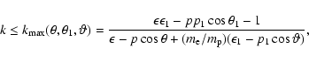
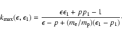
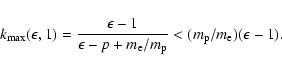
Energy and momentum of the
outgoing particles are designated by primed quantities. In order to
calculate the maximum photon energy,
.
Energy and momentum of the
outgoing particles are designated by primed quantities. In order to
calculate the maximum photon energy,
![]() ,
the finite rest mass of
the proton has to be taken into account. Otherwise
,
the finite rest mass of
the proton has to be taken into account. Otherwise
![]() could be
greater than the proton kinetic energy E for
could be
greater than the proton kinetic energy E for
![]() ,
in
contradiction to energy conservation (Heristchi 1986). In an arbitrary
frame of reference the conservation of energy and momentum is most
conveniently expressed in terms of the four-momenta which are denoted
by underlined quantities. Taking into account the different energy units
for protons, electrons, and photons the relation reads
,
in
contradiction to energy conservation (Heristchi 1986). In an arbitrary
frame of reference the conservation of energy and momentum is most
conveniently expressed in terms of the four-momenta which are denoted
by underlined quantities. Taking into account the different energy units
for protons, electrons, and photons the relation reads
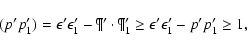
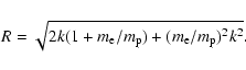
Solving Eq. (7) for ![]() and p leads to the minimum energy
and momentum, respectively, of the proton required to produce photons
of energy k. In the following we will restrict to the case that the
target electron is at rest in the laboratory system, i.e.,
and p leads to the minimum energy
and momentum, respectively, of the proton required to produce photons
of energy k. In the following we will restrict to the case that the
target electron is at rest in the laboratory system, i.e.,
![]() .
Then we have
.
Then we have
For
![]() ,
Eqs. (10) and (11) reduce to
,
Eqs. (10) and (11) reduce to
We consider the collision of an energetic proton with a stationary
electron (p1=0). Designating the variables in the proton rest system
by an asterisk, the invariance of the four-product (pk) yields
Using the relativistic transformation formula for the photon emission
angle ![]() ,
,
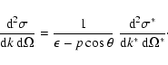
It is instructive to compare the differential cross section (18)
with that of the normal electron-proton bremsstrahlung where the electron
has the same velocity, i.e.,
![]() .
One notes the following: at
low proton energies the behaviour of the two cross sections is similar.
If the energies become higher, this changes drastically. The
electron-proton cross section has a sharp maximum at small angles
originating from the denominator
.
One notes the following: at
low proton energies the behaviour of the two cross sections is similar.
If the energies become higher, this changes drastically. The
electron-proton cross section has a sharp maximum at small angles
originating from the denominator
![]() .
Passing on to the rest frame of the proton, this expression transforms
to k so that the proton-electron cross section becomes more isotropic,
except for
.
Passing on to the rest frame of the proton, this expression transforms
to k so that the proton-electron cross section becomes more isotropic,
except for
![]() .
In any case protons can emit photons of higher
energy than electrons. For instance, protons of kinetic energy E=1 GeV
.
In any case protons can emit photons of higher
energy than electrons. For instance, protons of kinetic energy E=1 GeV
![]() produce photons of maximum energy
produce photons of maximum energy
![]() MeV, whereas electrons with the same velocity
MeV, whereas electrons with the same velocity
![]() keV) generate photons with
keV) generate photons with ![]() .
.
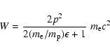
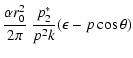
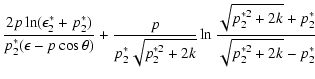
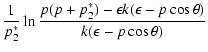
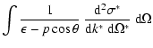
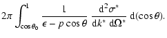
The spectrum integrated over the photon angles is given by
In the case
![]() one has to take the limit
one has to take the limit
In the cross section (18) the distortion of the electron wave
functions by the proton's Coulomb field is neglected. This can be taken
into account approximately if (18) is multiplied by the Elwert
factor (Elwert 1939; Elwert & Haug 1969)
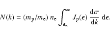
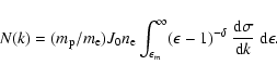
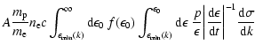
In a thin target the energy distribution of the incident protons is not
influenced by collisions with other particles. Denoting the spectral flux
of the protons by
![]() ,
the PEB photon spectrum (number of
photons emitted per second, cm3, and MeV) in a plasma with the ambient
electron density
,
the PEB photon spectrum (number of
photons emitted per second, cm3, and MeV) in a plasma with the ambient
electron density
![]() ,
assumed to be uniform, is given
by
,
assumed to be uniform, is given
by
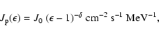
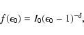
In many astrophysical applications
![]() has the form of a
power law in the kinetic energy with spectral index
has the form of a
power law in the kinetic energy with spectral index ![]() ,
,
The upper curve of Fig. 2 shows the photon energy distribution for the
spectral index
![]() of the cosmic-ray protons. At low photon
energies k<0.07, corresponding to
of the cosmic-ray protons. At low photon
energies k<0.07, corresponding to ![]() keV, the spectrum has
also the form of a power law with spectral index
keV, the spectrum has
also the form of a power law with spectral index
![]() ,
in agreement with Eq. (35). If k increases, the photon spectrum
flattens due to relativistic effects, and the spectral index becomes
,
in agreement with Eq. (35). If k increases, the photon spectrum
flattens due to relativistic effects, and the spectral index becomes
![]() for k>10 or
for k>10 or ![]() MeV. Inclusion of the Coulomb
correction factor (31) would change the photon flux a little at
low energies k. However, the slope of the spectrum is virtually the
same.
MeV. Inclusion of the Coulomb
correction factor (31) would change the photon flux a little at
low energies k. However, the slope of the spectrum is virtually the
same.
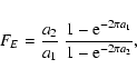
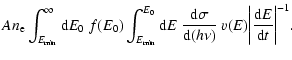
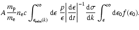
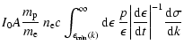
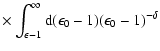
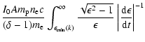
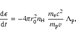
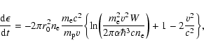
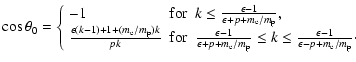
In a thick target the impinging protons are slowed down by collisions
with ambient particles. Employing normal energy units, the number of
photons of energy ![]() emitted by protons with the initial kinetic
energy E0 is
emitted by protons with the initial kinetic
energy E0 is
![\begin{figure}
\par\includegraphics[width=7.5cm,clip]{3991f2.eps}
\end{figure}](/articles/aa/full/2003/28/aa3991/img163.gif) |
Figure 2:
PEB photon spectra from protons with a power-law spectrum,
spectral index
|
The thick-target photon spectrum plotted in Fig. 2 was calculated for
a completely ionized hydrogen target with electron number density ![]() using the energy loss rate (Lang 1980)
using the energy loss rate (Lang 1980)
![\begin{figure}
\par\includegraphics[width=8.8cm,clip]{3991f1.eps}
\end{figure}](/articles/aa/full/2003/28/aa3991/img35.gif)
![$\displaystyle \frac{1+k^2+2(m_{\rm e}/m_{\rm p})k+(m_{\rm e}/m_{\rm p})^2k^2}{[1+(m_{\rm e}/m_{\rm p})k]
(1-k)+kR},$](/articles/aa/full/2003/28/aa3991/img46.gif)
![$\displaystyle k~\frac{1+(m_{\rm e}/m_{\rm p})[2-k+(m_{\rm e}/m_{\rm p})k]}{k[1+(m_{\rm e}/m_{\rm p})k]
+(1-k)R},$](/articles/aa/full/2003/28/aa3991/img48.gif)

![$\displaystyle \biggl\{{1\over p}\Bigl[\epsilon^2+{\epsilon\over\epsilon-p\cos\theta}
-2(2\epsilon^2+1)\cos^2\theta\Bigr]$](/articles/aa/full/2003/28/aa3991/img65.gif)
![$\displaystyle k(p-\epsilon\cos\theta)+{p^2\over p_2^{*2}+2k}\bigl[k(p-\epsilon\cos\theta)
-p\bigr]$](/articles/aa/full/2003/28/aa3991/img66.gif)
![$\displaystyle \Bigl[1-2k+{k^2\over
p_2^{*2}+2k}\bigl\{k(\epsilon-p\cos\theta)^2+p(\epsilon\cos\theta-p)\bigr\}\Bigr]$](/articles/aa/full/2003/28/aa3991/img68.gif)
![$\displaystyle (k/p^2)(\epsilon-p\cos\theta)(5\epsilon+pk\cos\theta)\Bigr]
\biggr\},$](/articles/aa/full/2003/28/aa3991/img72.gif)
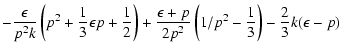
![$\displaystyle +{k\over 6p^2}(\epsilon+p)\biggr]$](/articles/aa/full/2003/28/aa3991/img91.gif)
![$\displaystyle +L_1(\epsilon-p)\biggl[{2\epsilon^2+3\over 12k^3}-{2\epsilon^2\over 3k^2}+{8\epsilon^2
\over 3k}+{1\over 6k}+{1\over 2}-{1\over 2k-1}\biggr]$](/articles/aa/full/2003/28/aa3991/img92.gif)
![$\displaystyle +2\int_{\epsilon-p}^{x_0}\biggl[(1-k){L_3(x)
\over W_2(x)}-{L_1(x)\over x}\biggr]~{\rm d}x\biggr\},$](/articles/aa/full/2003/28/aa3991/img97.gif)
![$\displaystyle \lim_{k\to 0.5}\biggl\{{1\over 2k-1}\bigl[2k~L_3(\epsilon-p)-L_1(\epsilon-p)
\bigr]\biggr\}$](/articles/aa/full/2003/28/aa3991/img108.gif)
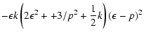
![$\displaystyle +{\displaystyle{2\over 3}}(\epsilon+p)k-{k\over 6p^2}(\epsilon-p)\biggr]-L_1(\epsilon+p)\biggl[{2\epsilon^2+3
\over 12k^3}-{2\epsilon^2\over 3k^2}$](/articles/aa/full/2003/28/aa3991/img114.gif)
![$\displaystyle +{8\epsilon^2\over 3k}+{1\over 6k}+{1\over 2}
-{1\over 2k-1}\biggr]$](/articles/aa/full/2003/28/aa3991/img115.gif)
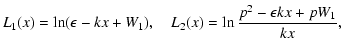
![$\displaystyle -{\epsilon k\over 2p^2}(\epsilon^2+2)(\epsilon+p)^4\biggr]+{2k\over 2k-1}~L_3(\epsilon+p)$](/articles/aa/full/2003/28/aa3991/img119.gif)
![$\displaystyle +2\int_{x_0}^{\epsilon+p}\biggl[(1-k){L_3(x)
\over W_2(x)}-{L_1(x)\over x}\biggr]~{\rm d}x
\biggr\}+{{\rm d}\sigma_1\over {\rm d}k}\cdot$](/articles/aa/full/2003/28/aa3991/img120.gif)
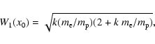
![$\displaystyle -{5\over p^2}-{1\over p^4}\biggr]
+k^2\biggl[{128\over 45}~\epsilon^2+{1307\over 45}-{5\over p^2}
-{4\over p^4}$](/articles/aa/full/2003/28/aa3991/img126.gif)
![$\displaystyle -{\epsilon\over 3p}\bigl(16p^2+6-1/p^2\bigr)\ln(\epsilon+p)
\biggr]\biggr\}.$](/articles/aa/full/2003/28/aa3991/img127.gif)