A&A 404, 997-1009 (2003)
DOI: 10.1051/0004-6361:20030528
T. Iijima1 - H. H. Esenoglu2,3
1 - Astronomical Observatory of Padova, Asiago
Section, Osservatorio Astrofisico, 36012 Asiago (Vi), Italy
2 -
Astronomy and Space Science Department of Istanbul University,
University Observatory, 34452, University, Istanbul, Turkey
3 -
Istanbul University Observatory Research and Application Center,
34452, University, Istanbul, Turkey
Received 28 January 2003 / Accepted 21 March 2003
Abstract
Spectral evolution of the fast nova V1494 Aql was monitored soon
after its discovery in December 1999 to September 2000. The first spectra
showed prominent emission lines of H I and Fe II, while He I was seen in
absorption. The radial velocities of the absorption components of H I,
He I and N II rapidly increased (in the negative sense) during the early
decline stage, while those of Fe II remained nearly constant. When a
new spectrum was taken on February 6, 2000 after the seasonal interruption,
this nova was in the transition stage. The spectra in the transition stage
showed emission lines of H I, He I, He II, N II, N III, Si II, [N II], [O I],
[O III], [Fe II], [Fe VI], [Ca V] etc., hence the emission lines of Fe II had
disappeared. A quasi-periodic oscillation of luminosity with a time scale of
about ![]() days and a mean amplitude of about 1.2 mag in V band was
seen from February to the middle of April 2000. The emission lines of He II
and [Ca V] disappeared around a light maximum of the oscillation, while the
emission lines of N II and N III strengthened. At the
same time high velocity (-2900 and +2830 km s-1) broad emission wings of
H I lines appeared, which suggest an ejection of high velocity jets.
The excitation state increased throughout the nebular stage. The last
spectra taken in September 2000 showed highly excited emission lines up to
[Fe VII] and [Fe X]
days and a mean amplitude of about 1.2 mag in V band was
seen from February to the middle of April 2000. The emission lines of He II
and [Ca V] disappeared around a light maximum of the oscillation, while the
emission lines of N II and N III strengthened. At the
same time high velocity (-2900 and +2830 km s-1) broad emission wings of
H I lines appeared, which suggest an ejection of high velocity jets.
The excitation state increased throughout the nebular stage. The last
spectra taken in September 2000 showed highly excited emission lines up to
[Fe VII] and [Fe X] ![]() 6374.5.
6374.5.
The interstellar extinction is estimated as
![]() from
the equivalent widths of the interstellar absorption components of Na I D1
and D2. Using this result, the distance to the nova is estimated as
from
the equivalent widths of the interstellar absorption components of Na I D1
and D2. Using this result, the distance to the nova is estimated as
![]() kpc. The mass and the helium abundance of the ejecta are
estimated as 6.2
kpc. The mass and the helium abundance of the ejecta are
estimated as 6.2 ![]() 1.4
1.4 ![]() 10
10
![]() and N(He)/N(H) = 0.13
and N(He)/N(H) = 0.13 ![]() 0.01, respectively. The electron density of the ejecta decreased as
0.01, respectively. The electron density of the ejecta decreased as
![]() during the nebular stage, where t is time
from light maximum. This low decline rate suggests that the ejecta had a
ring like shape as well a large mass loss which may have continued
throughout the nebular stage.
during the nebular stage, where t is time
from light maximum. This low decline rate suggests that the ejecta had a
ring like shape as well a large mass loss which may have continued
throughout the nebular stage.
Key words: stars: individual: V1494 Aql - novae, cataclysmic variables - ISM: general
V1494 Aql (Nova Aql 1999-II) was discovered by Pereira (1999) on
December 1, 1999 as a star of
![]() .
The luminosity and time
of light maximum were estimated as
.
The luminosity and time
of light maximum were estimated as
![]() on December 3.4 UT,
1999, JD 2 451 515.9, by Kiss & Thomson (2000). Early spectral evolution
was reported
by Kiss & Thomson (2000) and Anupama et al. (2001). Kiss
& Thomson (2000) obtained the decline rates of the luminosity
on December 3.4 UT,
1999, JD 2 451 515.9, by Kiss & Thomson (2000). Early spectral evolution
was reported
by Kiss & Thomson (2000) and Anupama et al. (2001). Kiss
& Thomson (2000) obtained the decline rates of the luminosity
![]() days and
days and
![]() days, and estimated the absolute
magnitude at maximum
days, and estimated the absolute
magnitude at maximum
![]() .
They obtained a
distance to the nova D = 3.6
.
They obtained a
distance to the nova D = 3.6 ![]() 0.3 kpc. This distance, however, should be
an upper limit because the effect of the interstellar extinction was not
taken into account. Kawabata et al. (2001) carried out some
spectro-polarimetric observations and suggested that the ejecta were not
spherically symmetric. Many coronal emission lines were detected by
infrared spectroscopy carried out in July 2000 (Venturini et al.
2000) and July 2001 (Rudy et al. 2001).
0.3 kpc. This distance, however, should be
an upper limit because the effect of the interstellar extinction was not
taken into account. Kawabata et al. (2001) carried out some
spectro-polarimetric observations and suggested that the ejecta were not
spherically symmetric. Many coronal emission lines were detected by
infrared spectroscopy carried out in July 2000 (Venturini et al.
2000) and July 2001 (Rudy et al. 2001).
The monitoring of spectral evolution of this nova in our observatory started soon after the announcement of discovery. The first spectra were taken on December 5, 1999, that is 2.3 days after maximum, then high and medium dispersion spectra were taken until September 16, 2000. In this paper, we report the spectral evolution of this nova in the early decline, transition, and nebular stages. The physical properties of the ejecta are estimated using the intensities of the emission lines in the nebular stage. The high velocity jets observed in the transition stage are also reported.
High dispersion spectra covering the range ![]()
![]() 4350-6900 Å with a
resolution of
4350-6900 Å with a
resolution of
![]() were taken with an Echelle
spectrograph mounted on the 182 cm telescope at the Mount Ekar station of
the Astronomical Observatory of Padova. Medium dispersion spectra were
taken with a Boller & Chivens grating spectrograph mounted on the 122 cm
telescope of the Astrophysical Observatory of Asiago of the University of
Padova. The resolution is
were taken with an Echelle
spectrograph mounted on the 182 cm telescope at the Mount Ekar station of
the Astronomical Observatory of Padova. Medium dispersion spectra were
taken with a Boller & Chivens grating spectrograph mounted on the 122 cm
telescope of the Astrophysical Observatory of Asiago of the University of
Padova. The resolution is
![]() with a
grating of 600 lines mm-1. The reductions of the spectra were carried out
using the standard tasks of the NOAO IRAF package at Asiago Observatory. The
spectrophotometric calibrations were made using the spectra of standard stars
taken in the same nights. HR 7596 (58 Aql) was used for the calibrations of
the high dispersion spectra and Kopff 27 for the medium dispersion spectra.
A log of the observations is given in Table 1, where UT is the universal time
at the start of the exposure and "days'' is number of days from light maximum.
with a
grating of 600 lines mm-1. The reductions of the spectra were carried out
using the standard tasks of the NOAO IRAF package at Asiago Observatory. The
spectrophotometric calibrations were made using the spectra of standard stars
taken in the same nights. HR 7596 (58 Aql) was used for the calibrations of
the high dispersion spectra and Kopff 27 for the medium dispersion spectra.
A log of the observations is given in Table 1, where UT is the universal time
at the start of the exposure and "days'' is number of days from light maximum.
The effect of interstellar extinction was not taken into account in the
previous works of this nova, because no interstellar absorption line was
detected in their low dispersion spectra (Kiss & Thomson 2000;
Anupama et al. 2001). The interstellar absorption components of Na I D1 and D2, however, are clearly seen on our high dispersion spectra (see,
e.g. Figs. 11-13). The mean equivalent widths of D1 and D2 are
![]() and
and
![]() Å, respectively. Using the double-ratio method of
Münch (1968), the column density of sodium atoms is estimated as
log(N(Na)L) =
Å, respectively. Using the double-ratio method of
Münch (1968), the column density of sodium atoms is estimated as
log(N(Na)L) =
![]() atoms cm-2 from these equivalent
widths, where L is the length of the line of sight in cm. The amount of
the interstellar extinction may be E(B-V) =
atoms cm-2 from these equivalent
widths, where L is the length of the line of sight in cm. The amount of
the interstellar extinction may be E(B-V) =
![]() and
and
![]() ,
where we adopted the chemical abundance of the interstellar
medium, log(N(Na)/N(H)) =-8.4 (Cohen 1975), and the relation between
the column density of hydrogen atom and the interstellar extinction,
N(H)L/E(B-V)
,
where we adopted the chemical abundance of the interstellar
medium, log(N(Na)/N(H)) =-8.4 (Cohen 1975), and the relation between
the column density of hydrogen atom and the interstellar extinction,
N(H)L/E(B-V)
![]() atoms cm
atoms cm
![]() (Jenkins & Savage 1974). The observed spectra are, therefore,
dereddened assuming E(B-V) =0.6.
(Jenkins & Savage 1974). The observed spectra are, therefore,
dereddened assuming E(B-V) =0.6.
If we add the effect of the interstellar extinction,
![]() ,
to
the result of Kiss & Thomson (2000), the distance to the nova should
be
,
to
the result of Kiss & Thomson (2000), the distance to the nova should
be
![]() kpc.
kpc.
![\begin{figure}
\par\includegraphics[width=8cm,clip]{3533fg01.eps}\end{figure}](/articles/aa/full/2003/24/aa3533/img27.gif) |
Figure 1: Light curve of V1494 Aql collected from VSNET (http://www.kusastro.kyoto-u.ac.jp/vsnet/index.html). |
Figure 1 shows the light curve of V1494 Aql collected from VSNET. This nova showed a fast fading in December 1999. Our first spectra were taken on December 5 with the Boller & Chivens spectrograph, then successive observations in the early decline stage were made on December 6 and 17.
Figures 2-4 show tracings of our first spectra, where the unit of the
ordinate is 10-10 erg cm-2 s-1 Å-1. Most prominent emission lines are of H I and Fe II, whereas He I and some N II lines are seen as absorptions. The weak
emission line at ![]() 6165.4 Å could be a blend of O I
6165.4 Å could be a blend of O I ![]() 6157.0 and N II
6157.0 and N II ![]() 6167.8 (Fig. 4). The emission components of H
6167.8 (Fig. 4). The emission components of H![]() ,
H
,
H![]() and H
and H![]() show single peak profiles, while H
show single peak profiles, while H![]() and some Fe II lines
show saddle shaped profiles. Some H I and Fe II lines are flanked by P Cygni
type absorption components. The absorption components of H
and some Fe II lines
show saddle shaped profiles. Some H I and Fe II lines are flanked by P Cygni
type absorption components. The absorption components of H![]() and H
and H![]() are very weak and that of H
are very weak and that of H![]() is not detected in our medium
dispersion spectra.
is not detected in our medium
dispersion spectra.
![\begin{figure}
\par\includegraphics[width=7.9cm,clip]{3533fg02.eps}\end{figure}](/articles/aa/full/2003/24/aa3533/img30.gif) |
Figure 2: A spectrum of V1494 Aql on Dec. 5, 1999. The unit of the ordinate is 10-10 erg cm-2 s-1 Å-1. |
![\begin{figure}
\par\includegraphics[width=7.9cm,clip]{3533fg03.eps}\end{figure}](/articles/aa/full/2003/24/aa3533/img31.gif) |
Figure 3: A spectrum of V1494 Aql on Dec. 5, 1999. The unit of the ordinate is 10-10 erg cm-2 s-1 Å-1. |
![\begin{figure}
\par\includegraphics[width=8cm,clip]{3533fg04.eps}\end{figure}](/articles/aa/full/2003/24/aa3533/img32.gif) |
Figure 4: A spectrum of V1494 Aql on Dec. 5, 1999. The unit of the ordinate is 10-10 erg cm-2 s-1 Å-1. |
The spectral features on December 6 were effectively the same as those on
December 5, while large changes were noticed on December 17. Figures 5-7
show tracings of the spectra on December 17. A tracing of the spectrum
multiplied by ten is over-plotted as a dotted line in Fig. 7 to reveal
the weak spectral features. In contrast to the earlier
spectra, H![]() and H
and H![]() show profiles with well separated two peaks
and a weak central peak. The emission components of H
show profiles with well separated two peaks
and a weak central peak. The emission components of H![]() and the higher
member of Balmer series are flanked by P Cygni type absorption components.
The blue-ward emission peaks of H
and the higher
member of Balmer series are flanked by P Cygni type absorption components.
The blue-ward emission peaks of H![]() and H
and H![]() seem to be cut
out by the absorption components. A weak trace of [O I]
seem to be cut
out by the absorption components. A weak trace of [O I] ![]() 5577.4 is seen on
the spectrum on December 17 (Fig. 6). This line was not seen on any other
earlier nor later spectra.
5577.4 is seen on
the spectrum on December 17 (Fig. 6). This line was not seen on any other
earlier nor later spectra.
An absorption line is seen at ![]() 4608 Å on the spectrum taken on December 17 (Fig. 5). If this line is due to N III
4608 Å on the spectrum taken on December 17 (Fig. 5). If this line is due to N III ![]() 4640.6, its radial velocity
should be -2110 km s-1. This velocity, however, is too low with respect to
those of the other N II and He I lines (see, Sect. 4.3). This absorption line
may be due to a blend of N III
4640.6, its radial velocity
should be -2110 km s-1. This velocity, however, is too low with respect to
those of the other N II and He I lines (see, Sect. 4.3). This absorption line
may be due to a blend of N III ![]() 4640.6, N II
4640.6, N II ![]() 4643.1 and O II
4643.1 and O II ![]() 4649.1.
4649.1.
![\begin{figure}
\par\includegraphics[width=7.9cm,clip]{3533fg05.eps}\end{figure}](/articles/aa/full/2003/24/aa3533/img33.gif) |
Figure 5: A spectrum of V1494 Aql on Dec. 17, 1999. The unit of the ordinate is 10-10 erg cm-2 s-1 Å-1. |
![\begin{figure}
\par\includegraphics[width=8.1cm,clip]{3533fg06.eps}\end{figure}](/articles/aa/full/2003/24/aa3533/img34.gif) |
Figure 6: A spectrum of V1494 Aql on Dec. 17, 1999. The unit of the ordinate is 10-10 erg cm-2 s-1 Å-1. |
![\begin{figure}
\par\includegraphics[width=8cm,clip]{3533fg07.eps}\end{figure}](/articles/aa/full/2003/24/aa3533/img35.gif) |
Figure 7: A spectrum of V1494 Aql on Dec. 17, 1999. The unit of the ordinate is 10-10 erg cm-2 s-1 Å-1. The dotted line shows a tracing of the spectrum multiplied by ten. |
The changes of the profiles of H![]() also have been reported in previous
works (Kiss & Thomson 2000; Anupama et al. 2001). The
observations made by Anupama et al. (2001) show that the profile
of H
also have been reported in previous
works (Kiss & Thomson 2000; Anupama et al. 2001). The
observations made by Anupama et al. (2001) show that the profile
of H![]() largely changed between December 10 and 16. When the profiles
of the H I lines changed, their widths significantly increased as shown in
Table 2.
largely changed between December 10 and 16. When the profiles
of the H I lines changed, their widths significantly increased as shown in
Table 2.
A weak emission line is seen at ![]() 7105 Å on the spectrum on December 17
(Fig. 7). This line was not observed in any previous novae or nova-like
objects, at far as we know. Its laboratory wavelength may be
7105 Å on the spectrum on December 17
(Fig. 7). This line was not observed in any previous novae or nova-like
objects, at far as we know. Its laboratory wavelength may be
![]() Å. Here, we tentatively identify it as [Ni II] 13F
Å. Here, we tentatively identify it as [Ni II] 13F ![]() 7102.8 (Moore
1959), but no other line of the same ion, e.g. [Ni II] 14F
7102.8 (Moore
1959), but no other line of the same ion, e.g. [Ni II] 14F ![]() 5275.8,
was detected in the spectra. Further works are necessary for the
identification of this line.
5275.8,
was detected in the spectra. Further works are necessary for the
identification of this line.
|
|
Elements | I( |
||
| (Å) | Dec. 5 | Dec. 6 | Dec. 17 | |
| 4108 | H |
75 | 80 | 46 |
| 4180 | Fe II 4179 | 36 | 42 | 8.0 |
| 4345 | H |
107 | 115 | 51 |
| 4637 | Fe II 4635 | 33 | 27 | 6: |
| 4647 | N II 4643, O II 4649 | 33 | ||
| 4863 | H |
231 | 219 | 101 |
| 4928 | Fe II 4924 | 55 | 47 | 16 |
| 5022 | Fe II 5018 | 71 | 64 | 30 |
| 5180 | Fe II 5169, N II 5176 | 74 | 60 | 11 |
| 5319 | Fe II 5317 | 8.4 | ||
| 5537 | Fe II 5535, N II 5535 | 14 | 11 | |
| 5576 | [O I] 5577.4 | 2.5 | ||
| 5902 | Fe II 5909, Na I, uid. | 16 | 12 | 4.6 |
| 6154 | Fe II 6149 | 2.4 | ||
| 6164 | N II 6168, O I 6157 | 15 | 10 | |
| 6247 | N II 6243, Fe II 6248 | 15 | 10 | 0.5: |
| 6316 | S II 6313 | 3.3 | ||
| 6568 | H |
411 | 429 | 607 |
| 6726 | [S II] 6717, 6731 | 2.7 | ||
| 7006 | O I 7002 | 2.3 | 0.9 | |
| 7105 | [Ni II] 7103? | 1.1 | ||
| H |
1.8 | 2.0 | 6.0 | |
| FWHM of H |
2420 | 2460 | 3120 | |
Unit of I(![]() )
is
)
is
![]() and that of FWHM is km s-1.
and that of FWHM is km s-1.
| Elements | Radial velocity in km s-1 | ||
| Dec. 5 | Dec. 6 | Dec. 17 | |
| H |
-1420 | -1460 | -2320 |
| H |
-1410 | -1520 | -2400 |
| Fe II 4403 | -1520 | -1490 | -1450 |
| He I 4471 | -1490 | -1580 | -2470 |
| Fe II 26, 4580 | -1570 | -1530 | -1470 |
| H |
-2450 | ||
| Fe II 49, 5235 | -1460 | -1450 | -1530 |
| Fe II 41, 5284 | -1520 | -1500 | |
| Fe II 48, 5338 | -1580 | -1540 | |
| Fe II 55, 5535 | -1540 | -1550 | |
| N II 3, 5667 | -1570 | -1650 | -2530 |
| N II 3, 5680 | -1620 | -1750 | -2590 |
| N II 3, 5711 | -1510 | -1660 | -2480 |
| N II 9, 5747 | -1540 | -1620 | -2450 |
| He I 5876 | -1560 | -1690 | -2560 |
| Na I D1+D2 | -1660 | ||
| O I 10, 6157 | -1610 | -1670 | -2240 |
| N II 36,60 6168 | -1600 | -1550 | -2520 |
| -1530 |
-1510 |
-1480 |
|
| -1560 |
-1640 |
-2510 |
|
| uid. | 4454.7 | 4454.4 | |
| uid. | 5868.3 | 5868.1 | 5870.5 |
uid.: wavelength of unidentified absorption line in Å.
Intensities after the correction of the interstellar extinction by
E(B-V)= 0.6 of some selected emission lines in December 1999 are given in
Table 2. The selected lines are relatively free from blending and are
not necessarily stronger than the others. The intensity ratio of H![]() /H
/H![]() and the FWHM of H
and the FWHM of H![]() are also presented. The
observational errors in the intensities are about
are also presented. The
observational errors in the intensities are about ![]() 10% and those in
the FWHM of H
10% and those in
the FWHM of H![]() are about
are about ![]() 50 km s-1. Intensities affected by larger
observational errors are denoted by a colon.
50 km s-1. Intensities affected by larger
observational errors are denoted by a colon.
Figure 8 shows the variation of the intensity ratio H![]() /H
/H![]() ,
where the results in the transition and nebular stages are also plotted. The
theoretical ratio of H
,
where the results in the transition and nebular stages are also plotted. The
theoretical ratio of H![]() /H
/H![]() in Case B recombination should be
found in the range of 2.6-3.0 in various conditions of electron temperature
and density (Hummer & Storey 1987). As seen in Fig. 8 and Table 2,
however, the ratio H
in Case B recombination should be
found in the range of 2.6-3.0 in various conditions of electron temperature
and density (Hummer & Storey 1987). As seen in Fig. 8 and Table 2,
however, the ratio H![]() /H
/H![]() of the present nova was lower than
the theoretical values on December 5 and 6. The ratio suddenly increased
afterwards and became much higher than the theoretical one on December 17.
At the same time, the profiles of H
of the present nova was lower than
the theoretical values on December 5 and 6. The ratio suddenly increased
afterwards and became much higher than the theoretical one on December 17.
At the same time, the profiles of H![]() and H
and H![]() significantly
changed and the width of H
significantly
changed and the width of H![]() increased, as reported in the previous
sub-section. The high intensity ratio continued until April 2000, then
gradually decreased (see also Sect. 6).
increased, as reported in the previous
sub-section. The high intensity ratio continued until April 2000, then
gradually decreased (see also Sect. 6).
The large ratios of H![]() /H
/H![]() on December 17 and later may not have
been due to an ejection of obscure matter, because a deep light minimum
such as of DQ Her (e.g. Martin 1989) was not seen in the light
curve of this nova (Fig. 1). Netzer (1975) called attention to the
effect of self-absorption of Lyman and Balmer photons in high density
nebulosity. Netzer (1975) showed that the ratio
H
on December 17 and later may not have
been due to an ejection of obscure matter, because a deep light minimum
such as of DQ Her (e.g. Martin 1989) was not seen in the light
curve of this nova (Fig. 1). Netzer (1975) called attention to the
effect of self-absorption of Lyman and Balmer photons in high density
nebulosity. Netzer (1975) showed that the ratio
H![]() /H
/H![]() from high density nebulosity are found in the range from 1.28 to 19.89 owing to the effect of self-absorption.
from high density nebulosity are found in the range from 1.28 to 19.89 owing to the effect of self-absorption.
When the optical depths of Lyman ![]() (
(
![]() )
and H
)
and H![]() (
(
![]() )
are very high, e.g.
)
are very high, e.g.
![]() and
and
![]() ,
we have low ratios of H
,
we have low ratios of H![]() /H
/H![]() similar
to those found on December 5 and 6. The intensity ratios higher than 4.0 are
found in some conditions of higher optical depth of Lyman
similar
to those found on December 5 and 6. The intensity ratios higher than 4.0 are
found in some conditions of higher optical depth of Lyman ![]() and/or
lower optical depth of H
and/or
lower optical depth of H![]() (Netzer 1975). It may be very
likely that the optical depths of Lyman
(Netzer 1975). It may be very
likely that the optical depths of Lyman ![]() and H
and H![]() were very
high in the earliest stage, and the effect of self-absorption was important.
The large variations of the ratio H
were very
high in the earliest stage, and the effect of self-absorption was important.
The large variations of the ratio H![]() /H
/H![]() could be explained
with this effect. A similar variation of the ratio H
could be explained
with this effect. A similar variation of the ratio H![]() /H
/H![]() was observed also in Nova (V1500) Cyg 1975 (Ferland 1978).
was observed also in Nova (V1500) Cyg 1975 (Ferland 1978).
Radial velocities of selected absorption lines are given in Table 3, where
![]() Fe II
Fe II![]() is the mean radial velocity of Fe II lines and
is the mean radial velocity of Fe II lines and ![]() He I+N II
He I+N II![]() is that of He I and N II lines. The observational errors in the
individual measurements are about
is that of He I and N II lines. The observational errors in the
individual measurements are about ![]() 100 km s-1. The radial velocities are
given in the frame of the nova system of which the receding velocity is
estimated as +46.3
100 km s-1. The radial velocities are
given in the frame of the nova system of which the receding velocity is
estimated as +46.3 ![]() 0.5 km s-1 measuring the line center of the emission
lines of [O III] and [N II] in the nebular stage. An absorption line at
0.5 km s-1 measuring the line center of the emission
lines of [O III] and [N II] in the nebular stage. An absorption line at ![]() 6125 Å on December 5 is identified as the O I multiplet No. 10 (Moore
1959). The weighted mean of the wavelengths of the three contiguous
lines of the multiplet is
6125 Å on December 5 is identified as the O I multiplet No. 10 (Moore
1959). The weighted mean of the wavelengths of the three contiguous
lines of the multiplet is ![]() 6157.03 Å.
6157.03 Å.
Figure 9 shows the mean radial velocities of the absorption components of H I, Fe II, and He I+N II. The radial velocities of H I, He I and N II rapidly increased (in negative sense) during the early decline stage. On the other hand, those of Fe II remained nearly constant or slightly decreased.
Increasing outflow velocity has been observed in many previous novae (e.g. McLaughlin 1960). This phenomenon may represent the increasing of escape velocity due to the shrink of the photosphere (see, e.g. the model of Kato & Hachisu 1994). The absorption lines of Fe II might have been due to a remnant of the spectrum at light maximum.
Kiss & Thomson (2000) estimated the expansion velocity of the ejecta
as 2000 km s-1 from their observations on December 8, but the outflow
velocity largely increased after their observations. The mean radial
velocity of He I and N II on December 17 was -2510 km s-1, and it seems that
the velocity was still increasing (in negative sense) at that time. The
outflow velocity may have increased up to about 2900 km s-1, because as shown
later high velocity jets having radial velocities of about ![]() 2900 km s-1
were observed in the transition stage (Sect. 5.2).
2900 km s-1
were observed in the transition stage (Sect. 5.2).
There were two unidentified absorption lines in the spectra of the early
decline stage. The wavelengths of the lines are given in Table 3. Since the
wavelengths did not change so much, these lines may be related to the group
of Fe II. If the radial velocities of these lines were the same as the
mean of Fe II lines, their laboratory wavelengths should be
![]()
![]() 1.0 and
1.0 and
![]()
![]() 1.0 Å, respectively. We are,
however, not able to find good candidates for these lines in the table of
Moore (1959).
1.0 Å, respectively. We are,
however, not able to find good candidates for these lines in the table of
Moore (1959).
One possible interpretation for these lines may be that the former line is
identified as He I ![]() 4471 blue-shifted by -1130 km s-1 on December 6 and -1150 km s-1 on December 17, and the latter is Na I D1+D2
4471 blue-shifted by -1130 km s-1 on December 6 and -1150 km s-1 on December 17, and the latter is Na I D1+D2 ![]() 5893
blue-shifted by -1260, -1270, and -1140 km s-1 on the respective days.
It is, however, required a detailed work for the structure of the atmosphere
of the nova to explain the reason why their radial velocities were so
different from those of the main absorption components of the same lines.
5893
blue-shifted by -1260, -1270, and -1140 km s-1 on the respective days.
It is, however, required a detailed work for the structure of the atmosphere
of the nova to explain the reason why their radial velocities were so
different from those of the main absorption components of the same lines.
We were not able to observe the nova in January 2000 because of its low celestial location. When the first spectrum in the new observational season was taken on February 6, 2000, this nova was in the transition stage. A large oscillation of luminosity, which is a typical phenomenon of the transition stage, was observed in the period from February to the middle of April 2000 (JD 2451570-1650) as seen in Fig. 1.
The spectroscopic observations in the transition stage were made on February 6, 21, March 7, 16 and 17. Figure 10 shows a tracing of the spectrum
on February 6. The prominent emission lines are of H I, He I, He II, N II, N III, and [O III], while the emission lines of Fe II had disappeared. A
weak emission line at ![]() 4245 Å is identified as [Fe II] 21F
4245 Å is identified as [Fe II] 21F ![]() 4244.8 Å. This nova may be one of rare fast novae which show [Fe II] lines like
CP Pup (Weaver 1944). The other lines of [Fe II] are blended
with stronger lines of other elements.
4244.8 Å. This nova may be one of rare fast novae which show [Fe II] lines like
CP Pup (Weaver 1944). The other lines of [Fe II] are blended
with stronger lines of other elements.
![\begin{figure}
\par\includegraphics[width=8.1cm,clip]{3533fg10.eps}\end{figure}](/articles/aa/full/2003/24/aa3533/img49.gif) |
Figure 10: A spectrum of V1494 Aql on Feb. 6, 2000. The unit of the ordinate is 10-10 erg cm-2 s-1 Å-1. |
![\begin{figure}
\par\includegraphics[width=8.1cm,clip]{3533fg11.eps}\end{figure}](/articles/aa/full/2003/24/aa3533/img50.gif) |
Figure 11: A high dispersion spectrum of V1494 Aql on Feb. 21, 2000. The unit of the ordinate is 10-10 erg cm-2 s-1 Å-1. The dotted line shows a tracing of the spectrum multiplied by ten. |
| Elements | I( |
|||||||
| Feb. 21 | Mar. 16 | Mar. 17 | Apr. 23 | Apr. 26 | May 15 | June 9 | Sep. 16 | |
| JD 2 451 000+ | 595.7 | 619.7 | 620.7 | 657.6 | 660.6 | 679.6 | 704.6 | 804.4 |
| [O III] 4363 | 6.5 | 5.7 | 4.2 | 4.5 | 4.3 | 4.3 | 3.5 | 0.92 |
| He I 4471 | 0.30 | 0.54 | 1.1 | 0.14 | 0.16 | 0.15 | ||
| N III 4511, 4515, 4524 | 0.58 | 0.40 | 2.8 | 0.31 | 0.22 | 0.23 | 0.40 | |
| N II 4607, 4614 | 0.88 | 0.60 | 0.35 | 0.36 | 0.64 | 0.15 | ||
| N II+N III | 12.5 |
21.4 |
||||||
| N III 4641, 4634 etc. | 3.9 | 2.1 | 1.6 | 1.5 | 1.6 | 0.21 | ||
| He II 4686 | 1.8 | <0.02 | <0.02 | 1.4 | 0.86 | 0.87 | 1.34 | 0.19 |
| H |
5.6 | 5.1 | 5.6 | 2.5 | 2.1 | 1.9 | 1.7 | 0.25 |
| [Fe VII] 4942 | 0.1: | |||||||
| [O III] 4959 | 3.3 | 4.8 | 3.8 | 3.1 | 3.0 | 3.1 | 2.9 | 1.2 |
| [O III] 5007 | 11.0 | 14.7 | 11.2 | 9.5 | 9.2 | 9.7 | 8.8 | 3.4 |
| Si II 5056 | 0.28 | 0.09 | 0.08 | 0.08 | ||||
| [Fe VI] 5147 | 0.14 | 0.11 | 0.09 | 0.08 | 0.10 | 0.05 | ||
| [Fe VI] 5177, N II 5180 | 0.26 | 0.35 | 0.4: | 0.23 | 0.17 | 0.17 | 0.17 | 0.03 |
| [Fe VI] 5279, [Fe III] 5270 | 0.24 | 0.13 | 0.6: | 0.07 | 0.12 | 0.10 | 0.08 | 0.08 |
| [Ca V] 5309 | 0.15 | 0.13 | 0.09 | 0.10 | 0.06 | |||
| He II 5411 | 0.1: | 0.10 | 0.08 | 0.07 | 0.12 | 0.02 | ||
| N II 5535 | 0.12: | 0.40 | 1.04 | 0.04 | 0.04 | 0.04 | ||
| [Ca VII] 5616 | 0.02 | |||||||
| N II 5667 | 0.26 | 0.32 | 0.6: | 0.11 | ||||
| N II 5680, [Fe VI] 5678 | 0.26 | 0.57 | 0.6: | 0.21 | 0.23* | 0.24* | 0.25* | 0.03* |
| [Fe VII] 5721 | 0.12 | |||||||
| [N II] 5755 | 2.5 | 3.2 | 5.0 | 1.14 | 1.24 | 1.05 | 0.76 | 0.15 |
| He I 5876 | 1.13 | 1.50 | 1.27 | 0.47 | 0.35 | 0.28 | 0.26 | 0.02 |
| N II 5940, 5942 | 0.28 | 0.20 | 0.38 | 0.08 | 0.06 | 0.07 | 0.06 | |
| [Ca V] 6086 | 0.28 | 0.27 | 0.21 | 0.22 | 0.22 | 0.19** | ||
| N II 6168 | 0.11 | 0.17 | 0.13 | |||||
| uid. |
0.02 | |||||||
| [O I] 6300, [S III] 6310 | 0.46 | 0.13 | 0.05 | 0.12 | 0.15: | 0.03 | 0.02 | |
| Si II 6347, 6371 | 0.48 | 0.17 | 0.18 | 0.19 | 0.05 | |||
| [Fe X] 6375 | 0.06 |
|||||||
| N II 6482 | 0.18 | 0.14 | 0.08 | 0.11 | 0.07 | 0.03 | ||
| H |
24.8 | 26.4 | 26.9 | 11.4 | 8.2 | 6.9 | 6.0 | 0.92 |
| [N II] 6584 | 0.49 | 0.63 | 0.62 | 0.33 | 0.28 | 0.26 | 0.21 | 0.07 |
| He I 6678 | 0.31 | 0.30 | 0.38 | 0.17 | 0.11 | 0.11 | 0.11 | |
| H |
4.4 | 5.2 | 4.8 | 4.6 | 3.9 | 3.7 | 3.5 | 3.7 |
| FWHM of H |
2730 | 2740 | 2710 | 2720 | 2710 | 2700 | 2720 | 2690 |
|
Unit of I( *: blended with N II |
| Elements | I( |
||
| Feb. 6 | Mar. 7 | Sep. 9 | |
| JD 2 451 000+ | 580.7 | 610.7 | 797.3 |
| [Fe VI] 4072, [S II] 4076 | 0.95 | 0.64 | 0.04 |
| H |
6.0 | 3.7 | 0.36 |
| N III 4196, 4200, He II 4200 | 0.30 | 0.17 | 0.04 |
| [Fe II] 4245 | 0.10 | ||
| H |
4.8 | 3.2 | 0.22 |
| [O III] 4363 | 8.1 | 9.9 | 2.2 |
| He I 4471 | 0.76 | 0.46 | 0.03 |
| N III 4511, 4515, 4524 | 0.78 | 0.54 | 0.12 |
| N II 4607 | 1.5 | 0.98 | 0.22 |
| N III 4634, 4641, 4642 | 7.0 | 4.3 | 0.37 |
| He II 4686 | 2.2 | 1.5 | 0.39 |
| S II 4792 | 0.04 | 0.03 | |
| N II 4803 | 0.07 | 0.03 | |
| H |
12.3 | 6.0 | 0.45 |
| [O III] 4959 | 4.1 | 4.6 | 2.5 |
| [O III] 5007 | 11.9 | 13.6 | 6.8 |
| S II 5056 | 0.53 | 0.29 | 0.02 |
| [Fe VI] 5147 | 0.04 | ||
| [Fe VI] 5177 | 0.08 | ||
| [Fe VII] 5721 | 0.20 | ||
| [N II] 5755 | 0.35 | ||
| He I 5876 | 0.04 | ||
| [Fe VII] 6086, [Ca V] 6086 | 0.24 | ||
| uid. |
0.02 | ||
| [O I] 6300, [S III] 6310 | 0.05 | ||
| [Fe X] 6375, Si II 6347 | 0.10 | ||
| N II 6482 | 0.03 | ||
| H |
1.40 | ||
| [N II] 6584 | 0.13 | ||
| He I 6678 | 0.01 | ||
| C II 6750 | 0.01 | ||
| [A V] 7006 | 0.03 | ||
| He I 7065 | 0.02 | ||
| [A III] 7136 | 0.03 | ||
| [A IV] 7236, C II 7231, 7236 | 0.01 | ||
| [O II] 7319, 7330 | 0.18 | ||
| H |
3.1 | ||
| FWHM of H |
2790 | 2790 | 2820 |
Unit of I(![]() )
is
)
is
![]() and that of FWHM is km s-1.
and that of FWHM is km s-1.
The first high dispersion spectrum with the Echelle spectrograph was taken
on February 21, 2000, whose tracing is shown in Fig. 11. A part of the
spectrum multiplied by ten is over-plotted as a dotted line to reveal
the faint spectral features. There are prominent emission lines of H I, He I,
He II, N II, N III, Si II, [O I], [O III], [N II], [Ca V] and [Fe VI]. The
emission line at ![]() 6086 Å is usually identified as a blend of [Ca V]
6086 Å is usually identified as a blend of [Ca V] ![]() 6085.9 and [Fe VII]
6085.9 and [Fe VII] ![]() 6085.5. In this spectrum, however, the emission line
may be due to [Ca V]
6085.5. In this spectrum, however, the emission line
may be due to [Ca V] ![]() 6085.9 alone, because no trace of [Fe VII]
6085.9 alone, because no trace of [Fe VII] ![]() 5721 is
seen. The emission lines of [Fe VII] were detected in September 2000 (Sect. 6.6). Intensities of prominent emission lines measured in the high dispersion
spectra in the transition and the nebular stages are summarized in Table 4,
and those measured in the medium dispersion spectra are given in Table 5.
The effect of the interstellar extinction is corrected assuming E(B-V)= 0.6.
Detailed process of the
decomposition of blended lines is given in Sect. 6.1. The observational
errors of the intensities of the prominent emission lines are about
5721 is
seen. The emission lines of [Fe VII] were detected in September 2000 (Sect. 6.6). Intensities of prominent emission lines measured in the high dispersion
spectra in the transition and the nebular stages are summarized in Table 4,
and those measured in the medium dispersion spectra are given in Table 5.
The effect of the interstellar extinction is corrected assuming E(B-V)= 0.6.
Detailed process of the
decomposition of blended lines is given in Sect. 6.1. The observational
errors of the intensities of the prominent emission lines are about ![]() 10%, and those of the weak lines, which means that the intensity is of the
order of
10%, and those of the weak lines, which means that the intensity is of the
order of
![]() ,
may be more than
,
may be more than ![]() 50%.
The intensities affected by larger errors are denoted by a colon.
50%.
The intensities affected by larger errors are denoted by a colon.
During the transition stage four light maxima of the oscillation were
observed at JD 2451587, 1606, 1621 and 1637 with an uncertainty of about ![]() 1 day. The interval between the maxima was 16.5
1 day. The interval between the maxima was 16.5 ![]() 1 days and the
mean amplitude of the oscillation was roughly 1.2 mag in V band. The
observations on February 6, 21 and March 7 were made near light minima of
the oscillation, while those on March 16 and 17 were made near the third
maximum at JD 2451621.
1 days and the
mean amplitude of the oscillation was roughly 1.2 mag in V band. The
observations on February 6, 21 and March 7 were made near light minima of
the oscillation, while those on March 16 and 17 were made near the third
maximum at JD 2451621.
Figures 12 and 13 show tracings of the high dispersion spectra taken on March 16 and 17, respectively. The spectral features near the light maximum were
significantly different from those at light minima (Figs. 10 and 11). The emission
complex at ![]() 4640 Å was already much stronger on March 16 (Fig. 12)
than on February 21 (Fig. 11), and its further large growth (nitrogen
flush) was observed on March 17 (Fig. 13). On the other hand, the emission
line of He II 4686 weakened near the maximum of the oscillation and was
embedded in the complex. The emission
complex at
4640 Å was already much stronger on March 16 (Fig. 12)
than on February 21 (Fig. 11), and its further large growth (nitrogen
flush) was observed on March 17 (Fig. 13). On the other hand, the emission
line of He II 4686 weakened near the maximum of the oscillation and was
embedded in the complex. The emission
complex at ![]() 4640 Å showed two broad peaks on March 17 (Fig. 13), of
which wavelengths were
4640 Å showed two broad peaks on March 17 (Fig. 13), of
which wavelengths were ![]() 4610 and
4610 and ![]() 4647 Å. The former may be due to N II
4647 Å. The former may be due to N II ![]()
![]() 4607.2 and 4613.9, while the latter may be a blend of N III
4607.2 and 4613.9, while the latter may be a blend of N III ![]()
![]() 4634.2,
4640.6, 4641.9, C III
4634.2,
4640.6, 4641.9, C III ![]()
![]() 4647.4, 4650.2, 4651.4 and probably O II
4647.4, 4650.2, 4651.4 and probably O II ![]() 4649.1 Å. In the red parts of the spectra the emission lines of N II appeared
or strengthened at light maximum, hence He II and [Ca V] disappeared (Figs. 12 and 13). Similar spectral variations were known on the other oscillating
novae GK Per and V603 Aql (see, e.g. McLaughlin 1943).
4649.1 Å. In the red parts of the spectra the emission lines of N II appeared
or strengthened at light maximum, hence He II and [Ca V] disappeared (Figs. 12 and 13). Similar spectral variations were known on the other oscillating
novae GK Per and V603 Aql (see, e.g. McLaughlin 1943).
![\begin{figure}
\par\includegraphics[width=8.1cm,clip]{3533fg12.eps}\end{figure}](/articles/aa/full/2003/24/aa3533/img54.gif) |
Figure 12: A high dispersion spectrum of V1494 Aql on March 16, 2000. The unit of the ordinate is 10-10 erg cm-2 s-1 Å-1. |
![\begin{figure}
\par\includegraphics[width=8.1cm,clip]{3533fg13.eps}\end{figure}](/articles/aa/full/2003/24/aa3533/img55.gif) |
Figure 13: A high dispersion spectrum of V1494 Aql on March 17, 2000. The unit of the ordinate is 10-10 erg cm-2 s-1 Å-1. |
The intensities of the forbidden lines also varied according
to the oscillation. McLaughlin (1943) reported that the intensity of [N II] ![]() 5755 increased and that of [O III]
5755 increased and that of [O III] ![]() 4363 decreased at light maxima
of the oscillation of V603 Aql. Similar variations were seen on the present
nova (Table 4). The intensity ratios of [O III] I(5007+4959)/I(4363) and [N II] I(6584+6548)/I(5755) suggest that the emitting region of [N II] lines
had higher temperature or higher density than that of [O III] lines at the
maximum of the oscillation. (Detailed arguments of these intensity ratios
are given in Sect. 6.2.)
4363 decreased at light maxima
of the oscillation of V603 Aql. Similar variations were seen on the present
nova (Table 4). The intensity ratios of [O III] I(5007+4959)/I(4363) and [N II] I(6584+6548)/I(5755) suggest that the emitting region of [N II] lines
had higher temperature or higher density than that of [O III] lines at the
maximum of the oscillation. (Detailed arguments of these intensity ratios
are given in Sect. 6.2.)
The profiles of N II ![]() 6167.8 and [N II]
6167.8 and [N II] ![]() 5755 on March 16 are shown in
Fig. 14. The emission line of [N II]
5755 on March 16 are shown in
Fig. 14. The emission line of [N II] ![]() 5755 shows well separated blue and red
peaks and some narrow smaller peaks around line center. Many prominent
emission lines show similar profiles (Figs. 12 and 13). On the other hand, the
emission line of N II
5755 shows well separated blue and red
peaks and some narrow smaller peaks around line center. Many prominent
emission lines show similar profiles (Figs. 12 and 13). On the other hand, the
emission line of N II ![]() 6167.8 shows only a featureless broad single peak.
Also the emission lines of N III may have had similar hazy profiles near
the light maximum, because no discrete peak was seen on the emission
complex at
6167.8 shows only a featureless broad single peak.
Also the emission lines of N III may have had similar hazy profiles near
the light maximum, because no discrete peak was seen on the emission
complex at ![]() 4640 Å (Figs. 12 and 13). The emission lines of N II and N III seem to have been formed in a more compact and nearly spherically symmetric
region.
4640 Å (Figs. 12 and 13). The emission lines of N II and N III seem to have been formed in a more compact and nearly spherically symmetric
region.
![\begin{figure}
\par\includegraphics[width=7.5cm,clip]{3533fg14.eps}\end{figure}](/articles/aa/full/2003/24/aa3533/img56.gif) |
Figure 14:
Profiles of [N II] |
The emission component of H![]() of V603 Aql at minimum of the oscillation
in the transition stage showed two well separated peaks, whereas a broad
single peak, which is rather similar to that of our N II
of V603 Aql at minimum of the oscillation
in the transition stage showed two well separated peaks, whereas a broad
single peak, which is rather similar to that of our N II ![]() 6167.8, was seen
at maximum (McLaughlin 1956). Such a large variation of the profiles
of H I lines was not observed in the present nova (Figs. 11-13).
6167.8, was seen
at maximum (McLaughlin 1956). Such a large variation of the profiles
of H I lines was not observed in the present nova (Figs. 11-13).
High velocity broad emission components appeared in the blue and red sides
of H![]() and H
and H![]() on March 16 and 17 (Figs. 12 and 13), namely near the light maximum of the oscillation. Figure 15 shows tracings of the H
on March 16 and 17 (Figs. 12 and 13), namely near the light maximum of the oscillation. Figure 15 shows tracings of the H![]() region of the spectra taken on March 16 and 17. The radial velocities of the
broad emission components in the frame of the nova system are given in Table 6. The observational errors are about
region of the spectra taken on March 16 and 17. The radial velocities of the
broad emission components in the frame of the nova system are given in Table 6. The observational errors are about ![]() 100 km s-1. The radial velocity of
the red component of H
100 km s-1. The radial velocity of
the red component of H![]() was not measured, because it was blended with
the emission line of [N II]
was not measured, because it was blended with
the emission line of [N II] ![]() 6584. The sum of the flux of the broad emission
components of H
6584. The sum of the flux of the broad emission
components of H![]() was roughly 3% of that of the main emission component
on March 16 and was about 6.5% on March 17.
was roughly 3% of that of the main emission component
on March 16 and was about 6.5% on March 17.
| March 16 | March 17 | |
| (km s-1) | ||
| H |
-2460 | -2900 |
| H |
+2830 | +2830 |
| H |
-2590 | -2860 |
It seems that high velocity jets were ejected at the light maximum of the oscillation. At far as we know, however, no previous nova showed a similar phenomenon during the transition stage. Even in the detailed description of the spectral variations of oscillating novae in the transition stage (McLaughlin 1943), such a high velocity emission component was never mentioned.
Rather similar high velocity emission components of H I and He II lines have
been observed in super-soft X-ray sources, e.g.
![]() -6951
(Crampton et al. 1996) and
-6951
(Crampton et al. 1996) and
![]() (Becker et al. 1998). The
radial velocities of the high velocity emission components of the former
object were
(Becker et al. 1998). The
radial velocities of the high velocity emission components of the former
object were ![]() 3600 km s-1 (Crampton et al. 1996) and those of
the latter were about
3600 km s-1 (Crampton et al. 1996) and those of
the latter were about ![]() 800-900 km s-1 (Becker et al. 1998). The
high velocity emission components of these objects, however, lasted at least
several months keeping nearly the same velocities. On the other hand, the
intensity and radial velocity of the high velocity emission components of the
present nova were rapidly variable.
800-900 km s-1 (Becker et al. 1998). The
high velocity emission components of these objects, however, lasted at least
several months keeping nearly the same velocities. On the other hand, the
intensity and radial velocity of the high velocity emission components of the
present nova were rapidly variable.
At the present time, our knowledge of the high velocity emission components of classical novae seems to be too poor to understand their properties. Detailed observations of the spectral variations in transition stage of novae in the future are required.
The oscillation of luminosity in the transition stage terminated at the middle of April 2000 (Fig. 1). A tracing of the high dispersion spectrum taken on April 23 is shown in Fig. 16. Notable differences with respect to the spectrum on February 21 (Fig. 11) are growth of [O III] and [Ca V] lines relative to H I.
Almost all prominent emission lines showed saddle-shaped profiles in the transition (Figs. 10-13) and nebular (Fig. 16) stages. Therefore, it is not possible to decompose blended lines with the usual Gaussian fitting. In this paper, we estimated the intensities of individual components of blended lines with the following method.
Since many lines in a spectrum showed nearly the same profile, we used the
profile of H![]() as the standard, and measured the intensities in the
blue and red quarters of the emission component. For example, the
wavelengths of the two peaks of H
as the standard, and measured the intensities in the
blue and red quarters of the emission component. For example, the
wavelengths of the two peaks of H![]() on the spectrum shown in Fig. 16
are
on the spectrum shown in Fig. 16
are ![]() 4843.5 and
4843.5 and ![]() 4880.0 Å, respectively. The full width at zero
intensity of the emission component is about 1.4 times larger than the
separation of the two peaks, that is the wavelengths at zero intensity are
4880.0 Å, respectively. The full width at zero
intensity of the emission component is about 1.4 times larger than the
separation of the two peaks, that is the wavelengths at zero intensity are
![]() 4836.2 and 4887.3 Å. We measured the intensities in the blue quarter
4836.2 and 4887.3 Å. We measured the intensities in the blue quarter
![]()
![]() 4836.2-4849.0 and in the red quarter
4836.2-4849.0 and in the red quarter ![]()
![]() 4874.5-4887.3 of the
emission component, then compared them with the total intensity. The ratio
of the intensity in the blue quarter to the total one is 0.23 and that in the
red quarter is 0.24 in the present case. Fortunately, the blue or red quarter
of many blended lines were free from blending. In such cases, we were able
to estimate the intensities of individual components of blended lines by
this method. This method was not applied to N II and N III lines in the
transition stage, because their profiles were different to that of H
4874.5-4887.3 of the
emission component, then compared them with the total intensity. The ratio
of the intensity in the blue quarter to the total one is 0.23 and that in the
red quarter is 0.24 in the present case. Fortunately, the blue or red quarter
of many blended lines were free from blending. In such cases, we were able
to estimate the intensities of individual components of blended lines by
this method. This method was not applied to N II and N III lines in the
transition stage, because their profiles were different to that of H![]() (Figs. 12-14). The intensities of the prominent emission lines in
the transition and nebular stages are given in Tables 4 and 5.
(Figs. 12-14). The intensities of the prominent emission lines in
the transition and nebular stages are given in Tables 4 and 5.
![\begin{figure}
\par\includegraphics[width=8.1cm,clip]{3533fg16.eps}\end{figure}](/articles/aa/full/2003/24/aa3533/img60.gif) |
Figure 16: A high dispersion spectrum of V1494 Aql on April 23, 2000. The unit of the ordinate is 10-10 erg cm-2 s-1 Å-1. The dotted line shows a tracing of the spectrum multiplied by ten. |
As mentioned in Sect. 4.2, the high intensity ratio of H![]() /H
/H![]() lasted during the transition stage, then gradually decreased (Fig. 8). The
ratio H
lasted during the transition stage, then gradually decreased (Fig. 8). The
ratio H![]() /H
/H![]() observed on April 26 and later (Tables 4 and 5) is
rather close to those expected in the recombination theory (Hummer & Storey
1987). Probably, the effect of the self-absorption (Netzer
1975) became weak in that period. The properties of the ejecta,
therefore, are analysed using the spectra taken on and later than April 26,
2000.
observed on April 26 and later (Tables 4 and 5) is
rather close to those expected in the recombination theory (Hummer & Storey
1987). Probably, the effect of the self-absorption (Netzer
1975) became weak in that period. The properties of the ejecta,
therefore, are analysed using the spectra taken on and later than April 26,
2000.
Figure 17 shows the profiles of the emission lines of H![]() ,
[N II]
,
[N II] ![]() 5755 and [O III]
5755 and [O III] ![]() 5007 on May 15. As seen in the figure, these three
lines have the same detailed structures. It seems that these
lines were formed in nearby regions. The uniform electron temperature and
density of the emitting regions of these lines, therefore, could be a good
approximation for the ejecta of this nova in the nebular stage. If this is
the case, it is easy to obtain the electron temperature and density from
the intensity ratios of the nebular lines to the auroral lines of [O III]
and [N II]. Seaton (1975) gave the following formulae.
5007 on May 15. As seen in the figure, these three
lines have the same detailed structures. It seems that these
lines were formed in nearby regions. The uniform electron temperature and
density of the emitting regions of these lines, therefore, could be a good
approximation for the ejecta of this nova in the nebular stage. If this is
the case, it is easy to obtain the electron temperature and density from
the intensity ratios of the nebular lines to the auroral lines of [O III]
and [N II]. Seaton (1975) gave the following formulae.
| |
|||
| = | (1) | ||
| = | (2) |
![\begin{figure}
\par\includegraphics[width=7.5cm,clip]{3533fg17.eps}\end{figure}](/articles/aa/full/2003/24/aa3533/img69.gif) |
Figure 17:
Profiles of H |
| Date | April 26 | May 15 | June 9 | Sep. 9 | Sep. 16 | mean | unit |
| days | 144.7 | 163.7 | 188.7 | 281.4 | 288.5 | ||
| 10 600 | 10 700 | 10 700 | 10 900 | 10 600 | 10 700 |
K | |
| 9.4 | 8.7 | 7.8 | 5.8 | 5.2 | 106 cm-3 | ||
| He I 5876 C/R | 0.25 | 0.26 | 0.26 | 0.28 | 0.25 | ||
|
|
0.10 | 0.09 | 0.09 | 0.05 | 0.05 | ||
|
|
0.04 | 0.04 | 0.07 | 0.08 | 0.07 | ||
|
|
0.14 | 0.13 | 0.16 | 0.13 | 0.12 | 0.13 |
|
| m(H) | 4.7 | 4.6 | 4.7 | 1.5 | 1.0 | 4.7 |
|
| m(total) | 6.2 | 6.0 | 6.3 | 1.9 | 1.3 | 6.2 |
|
The electron temperature was nearly constant at 10 700 K during the nebular
stage. The variation of the electron density with time is shown in Fig. 18.
As seen in the figure, the electron density decreased smoothly with a decline
rate of
![]() ,
where t is number of days from
light maximum. This decline rate is much lower than that expected in the
spherically symmetric expansion
,
where t is number of days from
light maximum. This decline rate is much lower than that expected in the
spherically symmetric expansion
![]() .
The ejecta
might have a form of a ring and, probably, polar blobs such as those of V603 Aql (Weaver 1974), HR Del (Hutchings 1972), DQ Her
(Martin 1989) etc.
.
The ejecta
might have a form of a ring and, probably, polar blobs such as those of V603 Aql (Weaver 1974), HR Del (Hutchings 1972), DQ Her
(Martin 1989) etc.
Another possible cause of the low decline rate is a continuous mass outflow
in the nebular stage. The model of Kato & Hachisu (1994) shows that
if the mass of the white dwarf is less than 1.15 ![]() ,
significant
mass outflow will continue even more than 150 days after the explosion.
Probably also this effect could contribute to the low decline rate.
,
significant
mass outflow will continue even more than 150 days after the explosion.
Probably also this effect could contribute to the low decline rate.
As mentioned in Sect. 5.1, the intensity ratios of [O III] and [N II] lines at the light maximum of the oscillation in the transition stage were rather peculiar. If we assume that the electron temperature was 10 700 K in the transition stage, the intensity ratios of the lines on March 16 and 17 give higher densities in the emission region of [N II] than in the [O III] region. On the other hand, if we extrapolate the decline rate of the electron density in the nebular stage to the transition stage, the same intensity ratios give higher temperature in the [N II] region than in the [O III] region. In any case, the condition of the ejecta at the light maximum of the oscillation may have been different from the thermal equilibrium.
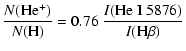
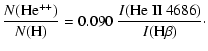
The helium abundance of the ejecta is estimated from the intensity ratios
of He I 5876/H![]() and He II 4686/H
and He II 4686/H![]() .
.
In the previous sub-section, we have found
![]()
![]() 106 cm-3 and
106 cm-3 and
![]() K for the ejecta in the nebular
stage. The effect of collisional excitation of He I 5876 can not be
neglected in such a nebulosity (Clegg 1987; Peimbert &
Torres-Peimbert 1987). Here, we use the formula of Peimbert &
Torres-Peimbert (1987) to estimate the ratio of
collision/recombination of He I 5876. The results are given as He I 5876 C/R
in Table 7. The effective recombination coefficients of H
K for the ejecta in the nebular
stage. The effect of collisional excitation of He I 5876 can not be
neglected in such a nebulosity (Clegg 1987; Peimbert &
Torres-Peimbert 1987). Here, we use the formula of Peimbert &
Torres-Peimbert (1987) to estimate the ratio of
collision/recombination of He I 5876. The results are given as He I 5876 C/R
in Table 7. The effective recombination coefficients of H![]() ,
He I 5876
and He II 4686 at
,
He I 5876
and He II 4686 at
![]() K and
K and
![]()
![]() 106 cm-3 are:
106 cm-3 are:
| (3) | |||
| (4) | |||
| (5) |
 |
(6) | ||
 |
(7) |
Following Osterbrock (1989), we have a relation between the
intensity of the H![]() emission line and the mass of hydrogen in the
emitting nebula of pure hydrogen as:
emission line and the mass of hydrogen in the
emitting nebula of pure hydrogen as:
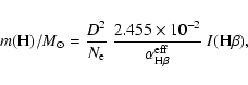 |
(8) |
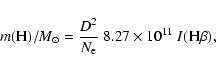 |
(9) |
 |
(10) |
| |
= | (11) | |
| = |   |
(12) |
If we assume that the ejecta has a uniform density, the mass of hydrogen
in the ejecta will be given as:
 |
(13) |
The radius of the ejecta on April 26 may be about 3.6 ![]() 1010 km,
where we assumed the expansion velocity of the ejecta to be 2900 km s-1. Using
the mass and the electron density given in Table 7, we have
1010 km,
where we assumed the expansion velocity of the ejecta to be 2900 km s-1. Using
the mass and the electron density given in Table 7, we have
![]() for April 26. The error in
for April 26. The error in ![]() is mainly due to the
uncertainty in the expanding velocity. If the error in the expanding velocity
is
is mainly due to the
uncertainty in the expanding velocity. If the error in the expanding velocity
is ![]() 200 km s-1, that in
200 km s-1, that in ![]() is about
is about ![]() 0.01. This factor was
0.022 on May 15 and 0.016 on June 9. These small factors also suggest that
the ejecta was not spherically symmetric, but may have had a ring-like shape.
0.01. This factor was
0.022 on May 15 and 0.016 on June 9. These small factors also suggest that
the ejecta was not spherically symmetric, but may have had a ring-like shape.
The low decline rate of the electron density (Sect. 6.2) and the small factor ![]() obtained in the previous sub-section suggest that the ejecta may
have had a ring-like form in the nebular stage. In addition to these results,
the widths of the emission lines seem to support the model of the ring-like
form of the ejecta.
obtained in the previous sub-section suggest that the ejecta may
have had a ring-like form in the nebular stage. In addition to these results,
the widths of the emission lines seem to support the model of the ring-like
form of the ejecta.
The outflow velocities measured with the blue-shifts of the absorption lines
in the early decline stage were larger than 2500 km s-1 (Fig. 9) and probably
reached up to 2900 km s-1 (Sect. 4.3). If the ejecta were expanding with such
velocities, the full widths of the emission lines in the nebular stage
should have been about 5000-6000 km s-1. On the other hand, the FWHMs of the
emission component of H![]() in the nebular stage were about 2700 km s-1 (Table 4) and the full width at zero intensity, which was measured on April 23 (Sect. 6.1), was 3200 km s-1. The widths of the other prominent emission
lines were nearly the same.
in the nebular stage were about 2700 km s-1 (Table 4) and the full width at zero intensity, which was measured on April 23 (Sect. 6.1), was 3200 km s-1. The widths of the other prominent emission
lines were nearly the same.
The disagreement between the radial velocities of the absorption lines and the widths of the emission lines could be explained if we assume that the ejecta in the nebular stage formed a ring which was expanding with the velocity of 2900 km s-1, but was inclined by about 30 degrees from the line of sight.
At the present time, three years after the explosion, the radius of the ejecta may be of order of 0.1 arcsec. This radius is large enough to be measured from ground based instruments or by the Hubble Space Telescope. Further works are awaited.
A tracing of a red spectrum taken on September 9 is shown in Fig. 19, where
the emission lines of [Fe VII] and the coronal line [Fe X] ![]() 6347 are seen.
Almost all prominent emission lines in the optical region (this paper) and
the coronal lines in the infrared region (Rudy et al. 2001) showed
double-peaked profiles, but the profile of [Fe X]
6347 are seen.
Almost all prominent emission lines in the optical region (this paper) and
the coronal lines in the infrared region (Rudy et al. 2001) showed
double-peaked profiles, but the profile of [Fe X] ![]() 6374 looks different. Its
strange profile may be due to a blending with Si II
6374 looks different. Its
strange profile may be due to a blending with Si II ![]() 6347. The FWHM of H
6347. The FWHM of H![]() was about 2700 km s-1 throughout the nebular stage (Table 4), and the
widths of the other prominent emission lines were nearly the same. If the
widths of Si II
was about 2700 km s-1 throughout the nebular stage (Table 4), and the
widths of the other prominent emission lines were nearly the same. If the
widths of Si II ![]() 6347 and [Fe X]
6347 and [Fe X] ![]() 6375 were also about 2700 km s-1, the red
part of Si II and the blue part of [Fe X] should overlap each other producing
a single strong peak between them. A similar profile of blended lines is seen
in the case of [Fe VI]
6375 were also about 2700 km s-1, the red
part of Si II and the blue part of [Fe X] should overlap each other producing
a single strong peak between them. A similar profile of blended lines is seen
in the case of [Fe VI] ![]()
![]() 5147 and 5177 on April 23 (Fig. 16)
5147 and 5177 on April 23 (Fig. 16)
Figure 20 shows a tracing of our last spectrum taken on September 16, 2000,
where [O III] ![]() 5007 is much stronger than H
5007 is much stronger than H![]() .
Like the spectrum
taken on September 9 (Fig. 19), some emission lines
of [Fe VII] and the coronal line [Fe X]
.
Like the spectrum
taken on September 9 (Fig. 19), some emission lines
of [Fe VII] and the coronal line [Fe X] ![]() 6347 are seen. No other coronal
line in the optical region, e.g. [Fe XIV]
6347 are seen. No other coronal
line in the optical region, e.g. [Fe XIV] ![]() 5304, is seen in this spectrum.
The same condition is known also in Nova (GQ) Mus 1983 (Krauter & Williams
1989). On the other hand, many coronal lines in the infrared
region, e.g. [Si VII], [Si X], [Ca VIII], [Al IX], [S IX] etc., were
observed in July 2000 (Venturini et al. 2000) and July 2001
(Rudy et al. 2001).
5304, is seen in this spectrum.
The same condition is known also in Nova (GQ) Mus 1983 (Krauter & Williams
1989). On the other hand, many coronal lines in the infrared
region, e.g. [Si VII], [Si X], [Ca VIII], [Al IX], [S IX] etc., were
observed in July 2000 (Venturini et al. 2000) and July 2001
(Rudy et al. 2001).
![\begin{figure}
\par\includegraphics[width=8.1cm,clip]{3533fg19.eps}\end{figure}](/articles/aa/full/2003/24/aa3533/img102.gif) |
Figure 19: A spectrum of V1494 Aql on September 9, 2000. The unit of the ordinate is 10-12 erg cm-2 s-1 Å-1. |
![\begin{figure}
\par\includegraphics[width=8cm,clip]{3533fg20.eps}\end{figure}](/articles/aa/full/2003/24/aa3533/img103.gif) |
Figure 20: A high dispersion spectrum of V1494 Aql on September 16, 2000. The unit of the ordinate is 10-12 erg cm-2 s-1 Å-1. |
The unidentified emission line at ![]() 6200, which was detected on CP Pup
(Sanford 1945), is seen on this nova (Figs. 19 and 20). Since this
line appeared in a later nebular stage, it may relate to a highly ionized
ion. Its precise laboratory wavelength should be
6200, which was detected on CP Pup
(Sanford 1945), is seen on this nova (Figs. 19 and 20). Since this
line appeared in a later nebular stage, it may relate to a highly ionized
ion. Its precise laboratory wavelength should be ![]() 6199.5
6199.5 ![]() 0.5 Å.
0.5 Å.
In this paper, a new distance 1.6 ![]() 0.2 kpc is derived for the nova
V1494 Aql. The mass of the ejecta is estimated as 6.2
0.2 kpc is derived for the nova
V1494 Aql. The mass of the ejecta is estimated as 6.2 ![]() 1.4
1.4 ![]()
![]() and the helium abundance as N(He)/N(H) =0.13
and the helium abundance as N(He)/N(H) =0.13 ![]() 0.01.
The electron temperature lasted nearly constant at 10 700 K during the
nebular stage, at least until the end of our monitoring in September 2000.
The electron density decreased as
0.01.
The electron temperature lasted nearly constant at 10 700 K during the
nebular stage, at least until the end of our monitoring in September 2000.
The electron density decreased as
![]() ,
where t
is number of days from light maximum. This low decline rate suggests that the
ejecta had a ring like form and that probably a significant mass outflow
continued in the nebular stage.
,
where t
is number of days from light maximum. This low decline rate suggests that the
ejecta had a ring like form and that probably a significant mass outflow
continued in the nebular stage.
This nova seems to be similar to V603 Aql in many aspects, e.g. the oscillation of luminosity in the transition stage, the spectral variations and the form of the ejecta. However, the high velocity jets observed around the light maximum of the oscillation in the transition stage have not been found in any previous nova. Careful spectroscopic observations in the transition stages of other novae are required to confirm the existence and better define the properties of the high velocity jets.
Acknowledgements
We are grateful to Profs. I. Hachisu and M. Kato for the useful discussions and comments, and to Prof. R. Barbon for the careful reading of the manuscript and useful suggestions. Thanks are also due to Dr. T. Kato, Dr. D. Nogami, Mr. S. Kiyota, and many other professional and amateur astronomers who supplied photometric data of V1494 Aql on the VSNET. HHE gratefully thanks both Italian Government Ministry of Foreign Affairs and the Research Fund of the University of Istanbul for financial support under a scholarship and the project 1506/280700.
| Date | UT | JD | Days | Exp. | Inst. | Range |
| s | nm | |||||
| 1999 | ||||||
| Dec. 5 | 17:27 | 518.23 | 2.3 | 180 | B&C | 350-465 |
| Dec. 5 | 17:53 | 120 | " | 400-515 | ||
| Dec. 5 | 18:00 | 60 | " | 490-610 | ||
| Dec. 5 | 18:15 | 10 | " | 590-710 | ||
| Dec. 5 | 18:16 | 30 | " | 590-710 | ||
| Dec. 6 | 17:35 | 519.23 | 3.3 | 180 | B&C | 400-515 |
| Dec. 6 | 17:54 | 120 | " | 490-610 | ||
| Dec. 6 | 18:01 | 10 | " | 590-700 | ||
| Dec. 6 | 18:02 | 30 | " | 590-700 | ||
| Dec. 17 | 17:09 | 530.21 | 14.3 | 120 | B&C | 400-515 |
| Dec. 17 | 17:26 | 120 | " | 480-600 | ||
| Dec. 17 | 17:36 | 10 | " | 600-720 | ||
| Dec. 17 | 17:37 | 60 | " | 600-720 | ||
| 2000 | ||||||
| Feb. 6 | 5:26 | 580.73 | 64.8 | 300 | B&C | 400-515 |
| Feb. 21 | 5:21 | 595.72 | 79.8 | 600 | Ech | 435-690 |
| Mar. 7 | 4:44 | 610.70 | 94.8 | 300 | B&C | 400-515 |
| Mar. 16 | 4:10 | 619.67 | 103.8 | 300 | Ech | 435-690 |
| Mar. 16 | 4:19 | 900 | " | " | ||
| Mar. 17 | 4:11 | 620.67 | 104.8 | 300 | " | " |
| Mar. 17 | 4:17 | 900 | " | " | ||
| Apr. 23 | 1:19 | 657.55 | 141.7 | 300 | " | " |
| Apr. 23 | 1:28 | 900 | " | " | ||
| Apr. 26 | 2:10 | 660.59 | 144.7 | 300 | " | " |
| Apr. 26 | 2:16 | 900 | " | " | ||
| May 15 | 1:48 | 679.57 | 163.7 | 300 | " | " |
| May 15 | 1:55 | 1200 | " | " | ||
| Jun. 9 | 1:10 | 704.55 | 188.7 | 600 | " | " |
| Jun. 9 | 1:22 | 1800 | " | " | ||
| Sep. 9 | 20:14 | 797.34 | 281.4 | 1200 | B&C | 400-515 |
| Sep. 9 | 21:35 | 600 | " | 570-690 | ||
| Sep. 9 | 21:56 | 600 | " | 620-740 | ||
| Sep. 16 | 20:53 | 804.37 | 288.5 | 600 | Ech | 435-690 |
| Sep. 16 | 21:05 | 1800 | " | " |
![\begin{figure}
\par\includegraphics[width=7.9cm,clip]{3533fg08.eps}\end{figure}](/articles/aa/full/2003/24/aa3533/img41.gif)
![\begin{figure}
\par\includegraphics[width=8.3cm,clip]{3533fg09.eps}\end{figure}](/articles/aa/full/2003/24/aa3533/img46.gif)
![\begin{figure}
\par\includegraphics[width=7cm,clip]{3533fg15.eps}\end{figure}](/articles/aa/full/2003/24/aa3533/img57.gif)
![\begin{figure}
\par\includegraphics[width=8.1cm,clip]{3533fg18.eps}\end{figure}](/articles/aa/full/2003/24/aa3533/img77.gif)