A&A 403, 817-828 (2003)
DOI: 10.1051/0004-6361:20030406
B. Ménard1,2 - T. Hamana3,1 - M. Bartelmann1 - N. Yoshida4,1
1 - Max-Planck-Institut für Astrophysik, PO Box 1317,
85741 Garching, Germany
2 -
Institut d'Astrophysique de Paris, 98 bis Bld Arago, 75014,
Paris, France
3 -
National Astronomical Observatory of Japan, Mitaka, Tokyo
181-8588, Japan
4 -
Harvard-Smithsonian Center for Astrophysics, 60 Garden Street,
Cambridge MA 02138, USA
Received 4 October 2002 / Accepted 17 March 2003
Abstract
The systematic magnification of background sources by the weak
gravitational-lensing effects of foreground matter, also called
cosmic magnification, is becoming an efficient tool both for
measuring cosmological parameters and for exploring the
distribution of galaxies relative to the dark matter. We extend
here the formalism of magnification statistics by estimating the
contribution of second-order terms in the Taylor expansion of the
magnification and show that the effect of these terms was previously
underestimated. We test our analytical predictions against numerical
simulations and demonstrate that including second-order terms allows
the accuracy of magnification-related statistics to be substantially
improved. We also show, however, that both numerical and analytical
estimates can provide only lower bounds to real correlation
functions, even in the weak lensing regime.
We propose to use count-in-cells estimators rather than
correlation functions for measuring cosmic magnification since they
can more easily be related to correlations measured in numerical
simulations.
Key words: cosmology: gravitational lensing - cosmology: large-scale structure of Universe
Gravitational lensing by large-scale structures magnifies sources and distorts their images. The systematic distortion of faint background galaxies near matter overdensities, the cosmic shear, has been measured by several groups in the past few years (Bacon et al. 2000, 2002; Hämmerle et al. 2002; Hoekstra et al. 2002; Kaiser et al. 2000; Maoli et al. 2001; Réfrégier et al. 2002; Rhodes et al. 2001; Van Waerbeke et al. 2000, 2001, 2002; Wittman et al. 2000). It was found to be in remarkable agreement with theoretical predictions based on the Cold Dark Matter model, and has already provided new constraints on cosmological parameters (Van Waerbeke et al. 2001).
In a similar way, systematic magnifications of background sources near foreground matter overdensities, the cosmic magnification, can be measured and can provide largely independent constraints on cosmological parameters (Ménard & Bartelmann 2002; Ménard et al. 2002). Gravitational magnification has two effects: first, the flux received from distant sources is increased, and the solid angle in which they appear is stretched, thus their density is diluted. The net result of these competing effects depends on how the loss of sources due to dilution is balanced by the gain of sources due to flux magnification. Sources with flat luminosity functions, like faint galaxies, are depleted by cosmic magnification, while the number density of sources with steep luminosity functions, like quasars, is increased. Thus, cosmic magnification gives rise to apparent angular cross-correlations between background sources and foreground matter overdensities which are physically completely uncorrelated with the sources. These overdensities can be traced by using the distribution of foreground galaxies.
Numerous studies have demonstrated the existence of quasar-galaxy correlations on angular scales ranging from one arcminute to about one degree, as expected from cosmic lensing (for a review, see Bartelmann & Schneider 2001; also Guimarães et al. 2001). In many cases, the measured correlation amplitudes have been higher than the theoretical predictions, however a number of non-detections have also been reported, leaving the true amplitude of the effect unclear from the observational point of view.
While cosmic shear can directly be related to observable quantities like image ellipticities, the theoretical interpretation of cosmic magnification involves several approximations:
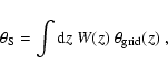
Our paper is structured as follows: first, we introduce the formalism of the effective magnification and its Taylor expansion in Sect. 2. We then describe a number of statistics related to the lensing convergence, and evaluate the amplitude of the second-order terms which appear in the Taylor expansion. In Sect. 3, we describe the numerical simulations we use to test our analytical results and estimate the accuracy of several approximations for the magnification. As an application, we investigate second-order effects on quasar-galaxy correlations in Sect. 4, and we summarise our results in Sect. 5.
Cosmic magnification can be measured statistically through characteristic changes in the number density of the background sources. Along a given line-of-sight, this effect depends on two quantities:
 |
(1) |
The local properties of the gravitational lens mapping are
characterised by the convergence ![]() ,
which is proportional to
the surface mass density projected along the line-of-sight, and the
shear
,
which is proportional to
the surface mass density projected along the line-of-sight, and the
shear ![]() ,
which is a two-component quantity and describes the
gravitational tidal field of the lensing mass distribution. The
effective magnification is related to
,
which is a two-component quantity and describes the
gravitational tidal field of the lensing mass distribution. The
effective magnification is related to ![]() and
and ![]() through
through
In doing so, we first note that
![]() and
and
![]() share the same statistical properties
(e.g. Blandford et al. 1991), because both
share the same statistical properties
(e.g. Blandford et al. 1991), because both ![]() and
and ![]() are
linear combinations of second-order derivatives of the lensing
potential. The identity of their statistics is most easily seen in
Fourier space. Since we will only deal with ensemble averages of the
magnification later on,
are
linear combinations of second-order derivatives of the lensing
potential. The identity of their statistics is most easily seen in
Fourier space. Since we will only deal with ensemble averages of the
magnification later on, ![]() and
and
![]() can be combined
into a single variable, which we denote by
can be combined
into a single variable, which we denote by ![]() for
simplicity. Thus, we can write for our purposes,
for
simplicity. Thus, we can write for our purposes,
![\begin{displaymath}\mu^{\alpha-1}=1+2(\alpha-1)\left[\kappa+\alpha\kappa^2\right]+
\mathcal{O}(\kappa^3)\;.
\end{displaymath}](/articles/aa/full/2003/21/aa3159/img35.gif) |
(4) |
![\begin{displaymath}P_{\mu^{\alpha-1}}(s)=4(\alpha-1)^2~\left[
P_\kappa(s)+2\alpha P_{\mu,2}(s)\right]\;;
\end{displaymath}](/articles/aa/full/2003/21/aa3159/img40.gif) |
(6) |
We will now estimate several ![]() -related statistical quantities
needed in the Taylor expansion of the magnification. For this purpose,
we first introduce the
-related statistical quantities
needed in the Taylor expansion of the magnification. For this purpose,
we first introduce the ![]() projector such that
projector such that
![\begin{displaymath}\kappa(\vec\theta)=\int_0^{w_{\rm H}}{\rm d}
w~p_\kappa(w)\delta\left[\vec\theta f_K(w),w\right]
\end{displaymath}](/articles/aa/full/2003/21/aa3159/img46.gif) |
(7) |
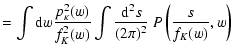
 |
(10) |
| |
= |  |
|
| (13) |
 |
(14) |
We can now numerically evaluate the first two contributions to the
Taylor expansion of the magnification autocorrelation function defined
in Eq. (5). As mentioned before, we use ![]() here.
here.
For evaluating the correlation functions, we use a CDM power spectrum
in a spatially flat Universe parameterised with
![]() ,
,
![]() ,
h=0.7 and
,
h=0.7 and
![]() .
The non-linear evolution of
the power spectrum and the bispectrum are computed according to the
formalisms developed by Peacock & Dodds (1996) and Scoccimarro et al. (2000), see Appendix A. The upper panel of
Fig. 1 shows the first- and second-order
contributions (dashed and dotted lines, respectively) to the Taylor
expansion of the magnification for a fixed source redshift of
.
The non-linear evolution of
the power spectrum and the bispectrum are computed according to the
formalisms developed by Peacock & Dodds (1996) and Scoccimarro et al. (2000), see Appendix A. The upper panel of
Fig. 1 shows the first- and second-order
contributions (dashed and dotted lines, respectively) to the Taylor
expansion of the magnification for a fixed source redshift of
![]() .
The sum of the two contributions is shown by the
solid line. The figure shows that the contribution of the second-order
term reaches an amplitude of more than 30% of the first-order term
on angular scales smaller than one arcminute. According to
Eq. (5) which describes the Taylor expansion of the
magnification autocorrelation, we define the contribution of
the second-order relative to the first-order term as
.
The sum of the two contributions is shown by the
solid line. The figure shows that the contribution of the second-order
term reaches an amplitude of more than 30% of the first-order term
on angular scales smaller than one arcminute. According to
Eq. (5) which describes the Taylor expansion of the
magnification autocorrelation, we define the contribution of
the second-order relative to the first-order term as
 |
(17) |
So far, we have only investigated the amplitude contributed by the
second-order term. In order to estimate the remaining contributions of
all missing terms of the magnification expansion, we will now use
numerical simulations allowing a direct computation of ![]() as a
function of the convergence
as a
function of the convergence ![]() and the shear
and the shear ![]() .
.
On sub-degree scales, lensing effects due to non-linearities in the density field can only be approximated using analytical fitting formulae (Peacock & Dodds 1996; Scoccimarro & Couchman 2001) as seen above. A full description requires numerical simulations (White & Hu 2000).
For testing the theoretical predictions we performed ray-tracing
experiments in a Very Large N-body Simulation (VLS) recently carried
out by the Virgo Consortium (Jenkins et al. 2001; and see also Yoshida
et al. 2001 for simulation details)![]() .
.
The simulation was performed using a parallel P3M code (MacFarland
et al. 1998) with a force softening length of
![]() .
The simulation employed 5123 CDM particles
in a cubic box of
.
The simulation employed 5123 CDM particles
in a cubic box of
![]() on a side. It uses a flat
cosmological model with a matter density
on a side. It uses a flat
cosmological model with a matter density
![]() ,
a
cosmological constant
,
a
cosmological constant
![]() ,
and a Hubble constant h=0.7. The initial matter power spectrum was computed using CMBFAST
(Seljak & Zaldarriaga 1996) assuming a baryonic matter density of
,
and a Hubble constant h=0.7. The initial matter power spectrum was computed using CMBFAST
(Seljak & Zaldarriaga 1996) assuming a baryonic matter density of
![]() .
The particle mass
(
.
The particle mass
(
![]() )
of the simulation
is sufficiently small to guarantee practically no discreteness effects
on dark-matter clustering on scales down to the softening length in
the redshift range of interest for our purposes (Hamana et al. 2002).
)
of the simulation
is sufficiently small to guarantee practically no discreteness effects
on dark-matter clustering on scales down to the softening length in
the redshift range of interest for our purposes (Hamana et al. 2002).
The multiple-lens plane ray-tracing algorithm we used is detailed in
Hamana & Mellier (2001; see also Bartelmann & Schneider 1992; Jain et al. 2000 for the theoretical basics); we thus
describe only aspects specific to the VLS N-body data in the
following. In order to generate the density field between z=0 and
![]() ,
we use a stack of ten snapshot outputs from two runs of the
N-body simulation, which differ only in the realisation of the
initial fluctuation field. Each cubic box is divided into 4 sub-boxes
of
,
we use a stack of ten snapshot outputs from two runs of the
N-body simulation, which differ only in the realisation of the
initial fluctuation field. Each cubic box is divided into 4 sub-boxes
of
![]() with the shorter box side
being aligned with the line-of-sight direction. The N-body particles
in each sub-box are projected onto the plane perpendicular to the
shorter box side and thus to the line-of-sight direction. In this way,
the particle distribution between the observer and
with the shorter box side
being aligned with the line-of-sight direction. The N-body particles
in each sub-box are projected onto the plane perpendicular to the
shorter box side and thus to the line-of-sight direction. In this way,
the particle distribution between the observer and ![]() is
projected onto 38 lens planes separated by
is
projected onto 38 lens planes separated by
![]() .
Note that in order to minimise the
difference in redshift between a lens plane and an output of N-body
data, only one half of the outputs (i.e. two sub-boxes) at z=0 are
used.
.
Note that in order to minimise the
difference in redshift between a lens plane and an output of N-body
data, only one half of the outputs (i.e. two sub-boxes) at z=0 are
used.
The particle distribution on each plane is converted into the surface density field on either a 10242 or 20482 regular grid using the triangular shaped cloud (TSC) assignment scheme (Hockney & Eastwood 1988). The two grid sizes are adopted for the following reasons:
We point out that second and higher-order statistics of point-source
magnifications are generally ill-defined in presence of caustic curves
because the differential magnification probability distribution
asymptotically decreases as ![]() for large
for large ![]() (see
Fig. 2). This is a generic feature of magnification near
caustics and is thus independent of the lens model. Strong lensing
effects on point sources near caustic curves give rise to rare, but
arbitrarily high magnification values in the simulations, and
therefore the variance of the measured statistics of
(see
Fig. 2). This is a generic feature of magnification near
caustics and is thus independent of the lens model. Strong lensing
effects on point sources near caustic curves give rise to rare, but
arbitrarily high magnification values in the simulations, and
therefore the variance of the measured statistics of ![]() cannot be
defined. However, the smoothing procedure introduced above allows this
problem to be removed because it smoothes out high density regions in
the dark matter distribution and thus the fractional area of high
magnification decreases. In reality, infinite magnifications do not
occur, for two reasons. First, each astrophysical source is extended
and its magnification (given the surface brightness-weighted
point-source magnification across its solid angle) remains
finite. Second, even point sources would be magnified by a finite
value since for them, the geometrical-optics approximation fails near
critical curves and a wave-optics description leads to a finite
magnification (Schneider et al. 1992, Chap. 7).
cannot be
defined. However, the smoothing procedure introduced above allows this
problem to be removed because it smoothes out high density regions in
the dark matter distribution and thus the fractional area of high
magnification decreases. In reality, infinite magnifications do not
occur, for two reasons. First, each astrophysical source is extended
and its magnification (given the surface brightness-weighted
point-source magnification across its solid angle) remains
finite. Second, even point sources would be magnified by a finite
value since for them, the geometrical-optics approximation fails near
critical curves and a wave-optics description leads to a finite
magnification (Schneider et al. 1992, Chap. 7).
The computation of correlation functions from numerical simulations is
mainly affected by two effects; on large scales by the finite box size
of the dark matter simulation, and on small scales by the grid size
used for computing the surface density field from the particle
distribution. These boundaries set the limits for the validity of
correlation functions measured in numerical simulations. In other
words, this means that measuring a correlation function on a given
scale is relevant only if this scale falls within the range of scales
defined by the simulation. As shown in the previous section, our
method for computing the cross-correlation between ![]() and
and ![]() consists of first computing a three-point correlation
function
consists of first computing a three-point correlation
function
![]() ,
and then identifying two of its
three points. In such a case, one of the correlation lengths of the
triple correlator becomes zero, thus necessarily smaller than the
smallest relevant scales in any simulation. This prevents us from
using any numerical simulation for directly comparing the results.
,
and then identifying two of its
three points. In such a case, one of the correlation lengths of the
triple correlator becomes zero, thus necessarily smaller than the
smallest relevant scales in any simulation. This prevents us from
using any numerical simulation for directly comparing the results.
In order to avoid this problem, and for comparing our analytical with
numerical results, we will introduce an effective smoothing into the
theoretical calculations, such that each value of ![]() at a given
position
at a given
position
![]() is evaluated by averaging the
is evaluated by averaging the ![]() -values in
a disk of radius
-values in
a disk of radius
![]() centred on
centred on
![]() .
Indeed, the limit imposed by the grid size of the simulation gives
rise to an unavoidable smoothing-like effect which cancels all
information coming from scales smaller than a corresponding smoothing
scale
.
Indeed, the limit imposed by the grid size of the simulation gives
rise to an unavoidable smoothing-like effect which cancels all
information coming from scales smaller than a corresponding smoothing
scale
![]() .
For this purpose, we introduce a
smoothed three-point correlator,
.
For this purpose, we introduce a
smoothed three-point correlator,
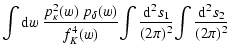
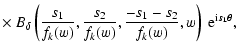
| (18) | |||
| |
= |  |
|
| (19) | |||
 |
![\begin{figure}
\par\includegraphics[width=8.8cm,clip]{smoothing.ps}
\end{figure}](/articles/aa/full/2003/21/aa3159/img114.gif) |
Figure 3:
Smoothing angle of the simulation as a function of redshift
for the two ray-tracing schemes. In order to show the relevant
quantities leading to the effective smoothing angle, we overplot the
weighting function
|
| small-scale smoothing | large-scale smoothing | |
|
|
|
|
|
|
|
|
The second important difference between analytical calculations and
measurements in numerical simulations is the finite box size
effect. Indeed, the analytical correlation functions presented above
were computed taking into account all modes in the power
spectrum. However, the finite size of the box used in the simulation
introduces an artificial cutoff in the power spectrum since
wavelengths larger than the box size are not sampled by the
simulation. This effect can also be taken into account in the
analytical calculations by simply cancelling all the power on
wavelengths with wave number
![]() .
The boxes we use have
a comoving size of
.
The boxes we use have
a comoving size of
![]() which corresponds to
which corresponds to
![]() .
.
With the help of the filtering schemes introduced in the previous section, we can now compare our theoretical predictions with correlation functions measured from the numerical simulations. We first compare the amplitude and angular variation of the two first terms of the Taylor expansion of the magnification separately. In the next section, we will then compare their sum to the total magnification fully computed from the simulation.
In Fig. 4, we overplot analytical and numerical
results. The upper curve shows the autocorrelation function of ![]() as a function of angular scale. We plot in circles the
average measurement from 36 realisations of the simulation, and the
corresponding 1-
as a function of angular scale. We plot in circles the
average measurement from 36 realisations of the simulation, and the
corresponding 1-![]() error bars to show the accuracy of the
numerical results as a function of angular scale. The solid line shows
the analytical prediction, including effective smoothing and an
artificial cut of the power at scales below
error bars to show the accuracy of the
numerical results as a function of angular scale. The solid line shows
the analytical prediction, including effective smoothing and an
artificial cut of the power at scales below
![]() .
The
agreement is good on all scales. For comparison, the dotted line shows
the result if we do not impose the large-wavelength cut, and the
dashed line is the result if no cut and no smoothing are applied. In
both cases, the deviations from the fully filtered calculation remain
small since we are probing angular scales within the range allowed by
the simulation.
.
The
agreement is good on all scales. For comparison, the dotted line shows
the result if we do not impose the large-wavelength cut, and the
dashed line is the result if no cut and no smoothing are applied. In
both cases, the deviations from the fully filtered calculation remain
small since we are probing angular scales within the range allowed by
the simulation.
The lower curves in Fig. 4 show a quantity
proportional to the second-order correction of the Taylor expansion,
namely the correlation function
![]() .
In
the same way as before, the circles show average measurements from 36 realisations, and the error bars denote the corresponding
1-
.
In
the same way as before, the circles show average measurements from 36 realisations, and the error bars denote the corresponding
1-![]() deviation. The prediction including smoothing and
small-wavelength cut (solid line) shows a relatively good agreement
given the expected accuracy of the bispectrum fitting formula, which
is approximately 15% (Scoccimarro & Couchman 2000). This time,
including smoothing changes the amplitude dramatically, and this
effect affects all scales (see the dashed line). As discussed before,
this is expected since we are measuring a three-point correlator on
triangles which have one side length smaller than the angular grid
size of the simulation. Finally, as shown by the difference between
the dotted and solid lines, cancelling the power on scales where
deviation. The prediction including smoothing and
small-wavelength cut (solid line) shows a relatively good agreement
given the expected accuracy of the bispectrum fitting formula, which
is approximately 15% (Scoccimarro & Couchman 2000). This time,
including smoothing changes the amplitude dramatically, and this
effect affects all scales (see the dashed line). As discussed before,
this is expected since we are measuring a three-point correlator on
triangles which have one side length smaller than the angular grid
size of the simulation. Finally, as shown by the difference between
the dotted and solid lines, cancelling the power on scales where
![]() again improves the agreement on large scales.
again improves the agreement on large scales.
The agreement between our analytical and numerical computations of
![]() and
and
![]() demonstrates the validity of the formalism introduced in
Sect. 2 as well as the choice of the effective smoothing
scale (Eq. (21)) for describing the second-order term
in the Taylor expansion of the magnification.
demonstrates the validity of the formalism introduced in
Sect. 2 as well as the choice of the effective smoothing
scale (Eq. (21)) for describing the second-order term
in the Taylor expansion of the magnification.
We now want to investigate how well the second-order expansion
describes the full magnification expression (2) which can
be computed using maps of ![]() ,
,
![]() and
and ![]() (a net
rotation term which arises from lens-lens coupling and the lensing
deflection of the light ray path; see Van Waerbeke et al. 2001b)
obtained from the simulations (see Hamana et al. 2000 for more
detail).
(a net
rotation term which arises from lens-lens coupling and the lensing
deflection of the light ray path; see Van Waerbeke et al. 2001b)
obtained from the simulations (see Hamana et al. 2000 for more
detail).
Before doing so, we recall that the amplitude of the magnification
autocorrelation measured from the simulation depends on the smoothing
scale, as seen in Sect. 3.2, since ![]() is nonlinear in
the density field. Therefore, all the following comparisons are valid
for a given effective smoothing length only.
is nonlinear in
the density field. Therefore, all the following comparisons are valid
for a given effective smoothing length only.
We further emphasise that two problems will complicate this
comparison. First, our analytical treatment is valid in the
weak-lensing regime only, i.e. as long as convergence and shear are
small compared to unity,
![]() ,
,
![]() .
While most
light rays traced through the numerical simulations are indeed weakly
lensed, a non-negligible fraction of them will experience
magnifications well above two, say. Such events are restricted to
small areas with high overdensities and thus affect the magnification
statistics only at small angular scales. Second, a separate problem
sets in if and where caustics are formed. The magnification of light
rays going through caustics is infinite, and the magnification
probability distribution near caustics drops like
.
While most
light rays traced through the numerical simulations are indeed weakly
lensed, a non-negligible fraction of them will experience
magnifications well above two, say. Such events are restricted to
small areas with high overdensities and thus affect the magnification
statistics only at small angular scales. Second, a separate problem
sets in if and where caustics are formed. The magnification of light
rays going through caustics is infinite, and the magnification
probability distribution near caustics drops like ![]() for
for
![]() .
As noted above, second- or higher-order statistics of
.
As noted above, second- or higher-order statistics of ![]() then become meaningless because they diverge.
then become meaningless because they diverge.
Departures of the numerical from the analytical results will thus have
two distinct reasons, viz. the occurrence of non-weak magnifications
which causes the analytical to underestimate the numerical results on
small angular scales; and the formation of caustics, which causes
second-order magnification statistics to break down entirely. Both
effects will be demonstrated below. They can be controlled or
suppressed in numerical simulations by smoothing, which makes lensing
weaker, or by masking highly magnified light rays or regions
containing caustics.
In Fig. 5, we plot with circles the autocorrelation
function
![]() measured from the large- and small-scale smoothing simulations in the
left and right panels, respectively. The presence of caustics is more
pronounced in the case of small-scale smoothing than in the
large-scale smoothing simulations. The dotted line shows the
theoretical prediction given by the first-order term of the Taylor
expansion, namely
measured from the large- and small-scale smoothing simulations in the
left and right panels, respectively. The presence of caustics is more
pronounced in the case of small-scale smoothing than in the
large-scale smoothing simulations. The dotted line shows the
theoretical prediction given by the first-order term of the Taylor
expansion, namely
![]() .
This
yields a low estimate of the correlation, with a discrepancy of order 10% on large scales, and more than 20% below a few arcminutes.
.
This
yields a low estimate of the correlation, with a discrepancy of order 10% on large scales, and more than 20% below a few arcminutes.
As expected from the preceding discussion, this level of discrepancy
also depends on the effective smoothing scale and can increase if
simulations with a smaller grid size are used. Estimating the
contribution of the two lowest-order terms of
![]() ,
we
computed in Sect. 2.3 a lower bound to this discrepancy
for a real case without smoothing, and found it to reach a level of 25% at large scales, and above 30% below a few arcminutes. The
smoothed results taking the additional contribution of the
second-order term into account are plotted as solid lines, and give a
much better agreement, as expected. To quantify this in more detail,
the lower panels of the figure show several contributions compared to
the first-order term, i.e. to
,
we
computed in Sect. 2.3 a lower bound to this discrepancy
for a real case without smoothing, and found it to reach a level of 25% at large scales, and above 30% below a few arcminutes. The
smoothed results taking the additional contribution of the
second-order term into account are plotted as solid lines, and give a
much better agreement, as expected. To quantify this in more detail,
the lower panels of the figure show several contributions compared to
the first-order term, i.e. to
![]() .
.
 |
(22) |
 |
(23) |
As the lower panel of the large-scale smoothing simulation shows, the
simple
![]() estimate of the magnification
misses 20% of the real amplitude near one arcminute. This
discrepancy almost vanishes after adding the contribution of the
second-order term, which gives at all scales a final agreement on the
per cent level: the additional amplitude reaches 19% at the smallest
scales of the figure, compared to a value of 20% given by the
simulation, and agrees within better than one per cent on larger
scales. Therefore, taking into account the
estimate of the magnification
misses 20% of the real amplitude near one arcminute. This
discrepancy almost vanishes after adding the contribution of the
second-order term, which gives at all scales a final agreement on the
per cent level: the additional amplitude reaches 19% at the smallest
scales of the figure, compared to a value of 20% given by the
simulation, and agrees within better than one per cent on larger
scales. Therefore, taking into account the
![]() correction allows the
accuracy to be increased by a factor of
correction allows the
accuracy to be increased by a factor of ![]() 20 compared to the
approximation
20 compared to the
approximation
![]() ,
in the case of our
large-scale smoothing simulation. On the largest scales,
between 6 and 30 arcmin, the agreement even improves. Above
these scales, the numerical results do not allow any relevant
comparison because the number of available independent samplings
corresponding to a given separation decreases. On scales below a few
arcminutes, the offset between the measured points and the analytical
estimate gives the amplitude of all higher-order terms neglected in
the Taylor expansion of the magnification. As we can see, their
contribution is on the one per cent level for the large-scale
smoothing simulation.
,
in the case of our
large-scale smoothing simulation. On the largest scales,
between 6 and 30 arcmin, the agreement even improves. Above
these scales, the numerical results do not allow any relevant
comparison because the number of available independent samplings
corresponding to a given separation decreases. On scales below a few
arcminutes, the offset between the measured points and the analytical
estimate gives the amplitude of all higher-order terms neglected in
the Taylor expansion of the magnification. As we can see, their
contribution is on the one per cent level for the large-scale
smoothing simulation.
The curves shown in the right panel demonstrate how the use of a smaller smoothing scale increases the discrepancy between the analytical and the numerical results. The fraction of non-weakly magnified light rays increases, and caustics appear which give rise to a power-law tail in the magnification probability distribution. We investigate the impact of the rare highly magnified light rays by masking pixels where the simulated magnification exceeds 4 or 8, and show that caustics have no noticeable effect on the amplitude of the magnification autocorrelation function determined from these simulated data. Note, however, that the impact of the caustics depends on the source redshift. The higher the redshift, the more caustics appear, and the larger is their impact on the correlation amplitude.
Imposing lower masking thresholds removes a significant fraction of
the area covered by the simulation, changing the spatial magnification
pattern and thus the magnification autocorrelation function. The
corresponding measurements are represented by the dashed error bars in
the lower right panel of Fig. 5. We note that the
error bars of
![]() computed with the small-scale
smoothing simulation become larger at small scales compared to the
lower left panel. This reflects the fact that second-order
magnification statistics are ill-defined once caustics appear. In the
next section, we will investigate similar smoothing effects on
cross-correlations between magnification and dark matter
fluctuations. These quantities are not affected by problems of poor
definition when the smoothing scale becomes small, and therefore do
not show larger error bars at small scales when the smoothing scale
decreases.
computed with the small-scale
smoothing simulation become larger at small scales compared to the
lower left panel. This reflects the fact that second-order
magnification statistics are ill-defined once caustics appear. In the
next section, we will investigate similar smoothing effects on
cross-correlations between magnification and dark matter
fluctuations. These quantities are not affected by problems of poor
definition when the smoothing scale becomes small, and therefore do
not show larger error bars at small scales when the smoothing scale
decreases.
These comparisons show that the approximation
![]() misses a non-negligible part of the total amplitude of weak-lensing
magnification statistics. The formalism introduced in
Sect. 2 allows second-order corrections to be described
with or without smoothing of the density field. This provides a better
description of the correlation functions, but still gives a lower
amplitude than the simulation results. As we noticed, the analytic
computation based on the Taylor expansion is sufficiently accurate
only in the weak lensing regime. In reality, however, the strong
lensing, which can not be taken into account in the analytic
formalism, has a significant impact on the magnification correlation
especially at small scales as shown in the small-scale smoothing
simulation. Therefore, one should carefully take the strong lensing
effect into consideration when one interprets the magnification
related correlation functions. However, we will see in the next
section that counts-in-cells estimators are less affected by the
strong lensing than correlation functions and thus enable better
comparisons of observations with results from simulations.
misses a non-negligible part of the total amplitude of weak-lensing
magnification statistics. The formalism introduced in
Sect. 2 allows second-order corrections to be described
with or without smoothing of the density field. This provides a better
description of the correlation functions, but still gives a lower
amplitude than the simulation results. As we noticed, the analytic
computation based on the Taylor expansion is sufficiently accurate
only in the weak lensing regime. In reality, however, the strong
lensing, which can not be taken into account in the analytic
formalism, has a significant impact on the magnification correlation
especially at small scales as shown in the small-scale smoothing
simulation. Therefore, one should carefully take the strong lensing
effect into consideration when one interprets the magnification
related correlation functions. However, we will see in the next
section that counts-in-cells estimators are less affected by the
strong lensing than correlation functions and thus enable better
comparisons of observations with results from simulations.
As a direct application of the formalism introduced previously, we now investigate the effects of second-order terms on a well-known magnification-induced correlation, namely the quasar-galaxy cross-correlation (the results can also be applied to galaxy-galaxy correlations induced by magnification; Moessner & Jain 1998). In order to estimate cosmological parameters from this kind of correlations, we then suggest the use of a more suitable estimator using counts-in-cells rather than two-point correlation functions. It has the advantage of making the observational results more easily reconciled with the ones from numerical simulations.
The magnification bias of large-scale structures, combined with galaxy biasing, leads to a cross-correlation of distant quasars with foreground galaxies. The existence of this cross-correlation has firmly been established (e.g. Benítez & Martínez-González 1995; Williams & Irwin 1998; Norman & Impey 1999; Norman & Williams 2000; Benítez et al. 2001; Norman & Impey 2001). Ménard & Bartelmann (2002) showed that the Sloan Digital Sky Survey (York et al. 2000) will allow this correlation function to be measured with a high accuracy. Its amplitude and angular shape contain information on cosmological parameters and the galaxy bias factor. Thus, it is important to accurately describe these magnification-related statistics in order to avoid a biased estimation of cosmological parameters as well as the amplitude of the galaxy bias.
As shown in Bartelmann (1995), the lensing-induced cross-correlation
function between quasars and galaxies can be written as
| |
|||
| = | (24) |
![\begin{displaymath}w_{\rm QG}(\theta)=2~(\alpha-1)~\left[
\langle\kappa\delta_{...
...le
+\alpha~\langle\kappa^2\delta_{\rm gal}\rangle
\right]\;.
\end{displaymath}](/articles/aa/full/2003/21/aa3159/img148.gif) |
(25) |
![\begin{displaymath}p_\delta(z)~{\rm d}z=\frac{\beta~z^2}{z_0^3~\Gamma(3/\beta)}~
\exp\left[-\left(\frac{z}{z_0}\right)^\beta\right]~{\rm d}z\;,
\end{displaymath}](/articles/aa/full/2003/21/aa3159/img156.gif) |
(27) |
The results are shown in Fig. 6. As we can see, previous
estimates using the approximation
![]() missed
approximately 15% of the amplitude on small scales for quasars at
redshift unity. Using quasars at redshift 2, these effects reach up
to 25%. These offsets, which are only lower limits, would lead to
biased estimates of
missed
approximately 15% of the amplitude on small scales for quasars at
redshift unity. Using quasars at redshift 2, these effects reach up
to 25%. These offsets, which are only lower limits, would lead to
biased estimates of ![]() or b, for example.
or b, for example.
As for the magnification autocorrelation, we can compare our
theoretical estimates against numerical estimations. We can first introduce
a coefficient
![]() describing the accuracy of our second-order
correction:
describing the accuracy of our second-order
correction:
 |
(28) |
For precisely estimating cosmological parameters as well as the amplitude of the galaxy bias, it is necessary to employ theoretical magnification statistics that closely describe the observables. However, we have seen in Sect. 3 that analytical estimates as well as numerical simulations have intrinsic limitations and prevent us from accurately describing usual n-point correlation functions related to magnification statistics.
Besides, it is possible to focus on another estimator closely related
to correlation functions, namely a count-in-cells estimator, which
naturally smoothes effects originating from the density field and can
thus more easily be reconciled with numerical simulations. So far,
quasar-galaxy or galaxy-galaxy correlations have been quantified
measuring the excess of background-foreground pairs at a given angular
separation. Instead, we can correlate the amplitude of the background
and foreground fluctuations, both measured inside a given aperture. We
will therefore introduce a count-in-cells estimator,
| |
= | ||
| (29) |
Using a first-order Taylor expansion for the magnification, the new
estimator
![]() can be written
can be written
 |
(30) |
In practice, masking always makes correlation functions easier to measure than counts-in-cells. However, in a large survey with short exposures like the SDSS, masking is not a real issue to measure counts-in-cells since unusable regions are quite rare and their area is small compared to the total survey size. This is different for cosmic shear surveys for which images are deeper and saturation occurs more frequently.
Note that gravitational lensing by the foreground galaxies themselves is entirely irrelevant here. The angular scale on which galaxies act as efficient lenses is on the order of one arc second and below, much smaller than the angular scales we are concerned with. Moreover, the probability for a quasar to be strongly lensed by a galaxy is well below one per cent. Bartelmann & Schneider (1991) demonstrated this point explicitly by including galaxies into their numerical simulations and showing they had no noticeable effect.
As surveys mapping the large-scale structure of the Universe become wider and deeper, measuring cosmological parameters as well as the galaxy bias with cosmic magnification will become increasingly efficient and reliable. Therefore, an accurate theoretical quantification of magnification statistics becomes increasingly important.
Previous estimates of cosmic magnification relied on the assumption
that the magnification deviates sufficiently little from unity that it
can be accurately approximated by its first-order Taylor expansion
about unity, i.e.
![]() .
In this paper, we have
tested the validity of this assumption in the framework of
magnification statistics, by investigating the second-order terms in
the Taylor expansion of
.
In this paper, we have
tested the validity of this assumption in the framework of
magnification statistics, by investigating the second-order terms in
the Taylor expansion of ![]() .
We have shown that:
.
We have shown that:
Using a simulation with an effective smoothing scale of 0.8 arcmin, we found that our second-order formalism is accurate to the
percent level for describing magnification autocorrelations. Compared
to previous estimates, this improves the accuracy by a factor of ![]() 20. For smaller effective smoothing scales, the contribution
of third- and higher-order terms becomes important on scales below a
few arcminutes.
20. For smaller effective smoothing scales, the contribution
of third- and higher-order terms becomes important on scales below a
few arcminutes.
Finally we have applied our formalism to observed correlations, like quasar-galaxy and galaxy-galaxy correlations due to lensing. We have shown that second-order corrections increase their amplitude by 15% to 25% on scales below one degree. These correlations are valuable tools to probe cosmological parameters as well as the galaxy bias. However, even including our correcting terms, analytical or numerical estimates of magnification statistics can only provide lower bounds to the real amplitude of the correlation functions in the weak-lensing regime. Thus, we propose using count-in-cells estimators rather than correlation functions since the intrinsic smoothing in determining counts-in-cells allows the observational results to be more directly related to those obtained in numerical simulations.
Thus, some care is required in using cosmic magnification as described by a Taylor expansion for constraining cosmological parameters, especially for interpreting measurements on small angular scales. Therefore, describing magnification statistics using the halo-model formalism will be of great interest in order to achieve a precise and direct description of observational quantities.
Acknowledgements
We thank Francis Bernardeau and Stéphane Colombi for helpful discussions. This work was supported in part by the TMR Network "Gravitational Lensing: New Constraints on Cosmology and the Distribution of Dark Matter'' of the EC under contract No. ERBFMRX-CT97-0172.
The bispectrum can be estimated using second-order perturbation
theory. Indeed, an expansion of the density field to second nonlinear
order as
 |
(A.1) |
The bispectrum
![]() is defined only for closed
triangles formed by the wave vectors
is defined only for closed
triangles formed by the wave vectors
![]() .
It can be
expressed as a function of the second-order kernel
.
It can be
expressed as a function of the second-order kernel
![]() and the power spectrum
and the power spectrum
| a(n,k) | = | ![$\displaystyle {1+\sigma_8^{-0.2}(z)\left[0.7~Q_3(n)\right]^{1/2}
(q/4)^{n+3.5}\over 1+(q/4)^{n+3.5}}$](/articles/aa/full/2003/21/aa3159/img197.gif) |
|
| b(n,k) | = |  |
|
| c(n,k) | = | ^{n+3}\over
1+(2q)^{n+3.5}},$](/articles/aa/full/2003/21/aa3159/img199.gif) |
(A.5) |
![\begin{displaymath}\mu^{\alpha-1}=\left[(1-\kappa)^2-\vert\gamma\vert^2\right]^{1-\alpha}\;,
\end{displaymath}](/articles/aa/full/2003/21/aa3159/img26.gif)
![\begin{displaymath}\mu^{\alpha-1}=1+(\alpha-1)\left[
2\kappa+(2\alpha-1)\kappa^...
...
\right]+\mathcal{O}\left(\kappa^3,\vert\gamma\vert^3\right).
\end{displaymath}](/articles/aa/full/2003/21/aa3159/img29.gif)
![\begin{figure}
\par\includegraphics[width=8.8cm,clip]{theoretical_kk.ps}
\end{figure}](/articles/aa/full/2003/21/aa3159/img75.gif)
![\begin{figure}
\par\includegraphics[width=8.8cm,clip]{pdf_mu3.ps}
\end{figure}](/articles/aa/full/2003/21/aa3159/img90.gif)
![\begin{figure}
\par\includegraphics[width=8.8cm,clip]{comparison_numerical.ps}
\end{figure}](/articles/aa/full/2003/21/aa3159/img127.gif)
![\begin{figure}
\par\includegraphics[width=8cm,clip]{comparison_mu_longshoot.ps} ...
...mm} \includegraphics[width=8cm,clip]{comparison_mu_raytrix_mask.ps}
\end{figure}](/articles/aa/full/2003/21/aa3159/img134.gif)
![\begin{figure}
\par\includegraphics[width=8.8cm,clip]{w_qg_corrected.ps}
\end{figure}](/articles/aa/full/2003/21/aa3159/img162.gif)
![\begin{figure}
\par\includegraphics[width=8.8cm,clip]{comparison_mu_delta.ps}
\end{figure}](/articles/aa/full/2003/21/aa3159/img166.gif)