A&A 403, 1123-1133 (2003)
DOI: 10.1051/0004-6361:20030385
A. A. Georgakilas 1 - E. B. Christopoulou 2 - A. Skodras 3,4 - S. Koutchmy 5
1 - Solar Astronomy, California Institute of Technology,
Pasadena, CA 91125, USA
2 -
Electronics Laboratory, University of Patras, Patras 26110,
Greece
3 -
School of Sciences and Technology, Hellenic Open University,
26222 Patras, Greece
4 -
Research Academic Computer Technology Institute, Riga Fereou 61,
26221 Patras, Greece
5 -
Institut d'Astrophysique de Paris, CNRS,
98 bis boulevard Arago, 75014 Paris, France
Received 10 September 2002 / Accepted 27 February 2003
Abstract
We studied the chromospheric Evershed flow from
filtergrams obtained at nine wavelengths along the H![]() profile.
We computed line-of-sight velocities based on Becker's cloud model and
we determined the components of the flow velocity vector as a function
of distance from the center of the sunspot, assuming an axial symmetry
of both the spot and the flow.
We found that the flow velocity decreases with decreasing height
and that the maximum of the velocity shifts
towards the inner penumbral boundary. The flow related to some fibrils
deviates significantly from the average Evershed flow. The profile of
the magnitude of the flow velocity as a function of distance from the
spot center, indicates that the velocity attains its maximum value in
the downstream part of the flow channels (assumed to have the form of a
loop). This behavior can be understood in terms of a critical flow that
pass from subsonic to supersonic near the apex of the loop, attains its
higher velocity at the downstream part of the loop and finally relaxes
to subsonic through a tube shock.
We computed the average flow vector from segmented line-of-sight velocity
maps, excluding bright or dark fibrils alternatively. We found that the
radial component of the velocity does not show a significant difference,
but the magnitude of the vertical component of the velocity related to
dark fibrils is higher than that related to bright fibrils.
profile.
We computed line-of-sight velocities based on Becker's cloud model and
we determined the components of the flow velocity vector as a function
of distance from the center of the sunspot, assuming an axial symmetry
of both the spot and the flow.
We found that the flow velocity decreases with decreasing height
and that the maximum of the velocity shifts
towards the inner penumbral boundary. The flow related to some fibrils
deviates significantly from the average Evershed flow. The profile of
the magnitude of the flow velocity as a function of distance from the
spot center, indicates that the velocity attains its maximum value in
the downstream part of the flow channels (assumed to have the form of a
loop). This behavior can be understood in terms of a critical flow that
pass from subsonic to supersonic near the apex of the loop, attains its
higher velocity at the downstream part of the loop and finally relaxes
to subsonic through a tube shock.
We computed the average flow vector from segmented line-of-sight velocity
maps, excluding bright or dark fibrils alternatively. We found that the
radial component of the velocity does not show a significant difference,
but the magnitude of the vertical component of the velocity related to
dark fibrils is higher than that related to bright fibrils.
Key words: Sun: sunspots - Sun: chromosphere - magnetohydrodynamics (MHD) - techniques: image processing
An important property of sunspot penumbrae at the photospheric level
is the well-known Evershed effect, a predominantly radial horizontal
outflow from the sunspot to the surroundings (see Muller 1992; Thomas 1994; Maltby 1997, for recent reviews).
At the chromospheric level around most mature sunspots a superpenumbra
is usually present. It consists of roughly radial elongated fibrils
that begin within the penumbra and extend a few spot radii beyond the
penumbra (Loughhead 1968; Moore 1981).
Inherent to the superpenumbra is a material flow directed towards the
sunspot umbra that is called the inverse Evershed flow. It is believed
to be a material flow along the superpenumbral fibrils, assumed to form
individual magnetic flux tubes. A siphon flow mechanism has been
proposed as an explanation; the driving force of the motion is the gas
pressure difference between the two foot points of a flux tube
(Meyer & Schmidt 1968; Maltby 1997; Thomas 1994).
Several authors studied the inverse Evershed flow, trying to determine
the basic characteristics of the flow.
Beckers (1964), using H![]() filtergrams, concluded that
the chromospheric material appears to flow into the spot along dark
"channels'' with a velocity of about 40-50 km s-1.
Haugen (1969), based on Doppler velocities determined
from H
filtergrams, concluded that
the chromospheric material appears to flow into the spot along dark
"channels'' with a velocity of about 40-50 km s-1.
Haugen (1969), based on Doppler velocities determined
from H![]() spectra, computed the radial and vertical components
of the flow. He found that the average velocity
vector shows a maximum of 6.8
spectra, computed the radial and vertical components
of the flow. He found that the average velocity
vector shows a maximum of 6.8 ![]() 1.2 km s-1 just outside the
penumbral rim and decreases quickly with increasing distance from
the spot. He found rms deviations of the order of 7 km s-1 from
the average velocity field.
1.2 km s-1 just outside the
penumbral rim and decreases quickly with increasing distance from
the spot. He found rms deviations of the order of 7 km s-1 from
the average velocity field.
Maltby (1975) studied the flow
using high-resolution filtergrams of a sunspot region observed at
seven wavelengths in H![]() and applying the photographic subtraction
method, in order to compute Dopplergrams. He concluded that the gas is
moving in flow channels that have the form of loops with cross section
changing with height and distance from the sunspot; the gas first moves
with a subsonic speed, obtains a supersonic speed close to the summit
of the loop and remains supersonic until it passes to subsonic through
a shock. Moore (1981) comparing H
and applying the photographic subtraction
method, in order to compute Dopplergrams. He concluded that the gas is
moving in flow channels that have the form of loops with cross section
changing with height and distance from the sunspot; the gas first moves
with a subsonic speed, obtains a supersonic speed close to the summit
of the loop and remains supersonic until it passes to subsonic through
a shock. Moore (1981) comparing H![]() filtergrams
concluded that the flow is concentrated along those fibrils which are
darkest in the line center and estimated the flow velocity to be about
20 km s-1.
filtergrams
concluded that the flow is concentrated along those fibrils which are
darkest in the line center and estimated the flow velocity to be about
20 km s-1.
Dialetis et al. (1985) and Dere et al. (1990) used
medium resolution filtergrams at 9 wavelengths along the H![]() line in order to study the phenomenon. They computed the components
of the velocity vector as a function of distance from the center of
the spot under the assumption of axial symmetry. They found
radial inflows of up to 2.6 km s-1 in the H
line in order to study the phenomenon. They computed the components
of the velocity vector as a function of distance from the center of
the spot under the assumption of axial symmetry. They found
radial inflows of up to 2.6 km s-1 in the H
![]() Å
chromosphere (Mach numbers of about 0.25) and that the maximum of the
velocity is well outside the penumbra. They proposed that the velocity
remains subsonic along the flux tubes.
Å
chromosphere (Mach numbers of about 0.25) and that the maximum of the
velocity is well outside the penumbra. They proposed that the velocity
remains subsonic along the flux tubes.
As it is clear from the previous short review there is a discrepancy
concerning the magnitude of the velocity and whether the flow can be
described as a critical or subcritical siphon flow. In this work we
study the chromospheric Evershed phenomenon, using high resolution
filtergrams at nine wavelengths along the H![]() profile. We compute
the velocity components of the average flow, trying to resolve the
above discrepancies and better understand the nature of the flow.
We further investigate the properties of the flow for different
categories of fibrils (bright/dark).
profile. We compute
the velocity components of the average flow, trying to resolve the
above discrepancies and better understand the nature of the flow.
We further investigate the properties of the flow for different
categories of fibrils (bright/dark).
Observations were obtained at the R.B. Dunn telescope of the Sacramento
Peak Observatory with a 512 by 512 pixel CCD camera and the UBF filter.
The pixel spatial resolution was 0.26
![]() .
A large isolated sunspot
was observed at N14.7, E26.0 on August 15, 1997. The observations are
described in detail in Christopoulou et al. (2001).
In this paper we focus our analysis on a sequence of filtergrams obtained
at 9 wavelengths along the H
.
A large isolated sunspot
was observed at N14.7, E26.0 on August 15, 1997. The observations are
described in detail in Christopoulou et al. (2001).
In this paper we focus our analysis on a sequence of filtergrams obtained
at 9 wavelengths along the H![]() profile (0,
profile (0, ![]() 0.35,
0.35,
![]() 0.5,
0.5, ![]() 0.75,
0.75, ![]() 1.0 Å). The duration of the observations
was about 10 min. The time interval between successive images of the
same wavelength was 36 s and the time difference between opposite
H
1.0 Å). The duration of the observations
was about 10 min. The time interval between successive images of the
same wavelength was 36 s and the time difference between opposite
H![]() wings was 4 s. The precision of the UBF filter is of
the order of 1 mÅ, while the FWHM is about 240 mÅ near H
wings was 4 s. The precision of the UBF filter is of
the order of 1 mÅ, while the FWHM is about 240 mÅ near H![]() .
Raw images were corrected for dark current
and flat field and carefully aligned. In order to align the images we
first computed spatially "enhanced'' images applying an image
enhancement method based on the "à trous" wavelet transform
(see Sect. 3.3 and Christopoulou et al. 2002). Subsequently we used
a cross correlation algorithm in order to compute the offset between two
images, based on the area of the superpenumbra. The displacements
computed this way were then applied to the original images.
.
Raw images were corrected for dark current
and flat field and carefully aligned. In order to align the images we
first computed spatially "enhanced'' images applying an image
enhancement method based on the "à trous" wavelet transform
(see Sect. 3.3 and Christopoulou et al. 2002). Subsequently we used
a cross correlation algorithm in order to compute the offset between two
images, based on the area of the superpenumbra. The displacements
computed this way were then applied to the original images.
![\begin{figure}
\par\includegraphics[width=7.1cm,clip]{3078f5a.eps}\par\vspace*{3mm}
\includegraphics[width=7.1cm,clip]{3078f5b.eps}\end{figure}](/articles/aa/full/2003/21/aa3078/img11.gif) |
Figure 5:
Comparison of the radial a) and the vertical b) components
of the line-of-sight velocity computed at H
|
![\begin{figure}
\par\includegraphics[width=7.5cm,clip]{3078f6.eps}\end{figure}](/articles/aa/full/2003/21/aa3078/img12.gif) |
Figure 6:
Comparison of the magnitude of the flow velocity at
H
|
Bray (1973b) introduced a method based on Becker's
cloud model (e.g. Beckers 1964) for the computation
of reliable line-of-sight velocities from opposite H![]() line wing
filtergrams. Becker's cloud model assumes that the chromospheric
features are cloud structures overlying a uniform stationary atmosphere.
The model takes into account four parameters: the
source function S, the optical depth at line center
line wing
filtergrams. Becker's cloud model assumes that the chromospheric
features are cloud structures overlying a uniform stationary atmosphere.
The model takes into account four parameters: the
source function S, the optical depth at line center
![]() ,
the
Doppler width
,
the
Doppler width
![]() which depends on the temperature
and the micro-turbulent motions, and the Doppler shift
which depends on the temperature
and the micro-turbulent motions, and the Doppler shift
![]() corresponding to the line-of-sight component of the velocity.
All parameters are assumed to be constant along the line-of-sight
through the structure. Furthermore, the source function is considered
wavelength-independent and the profile of the optical depth Gaussian.
According to the cloud model approximation the intensity
profile
corresponding to the line-of-sight component of the velocity.
All parameters are assumed to be constant along the line-of-sight
through the structure. Furthermore, the source function is considered
wavelength-independent and the profile of the optical depth Gaussian.
According to the cloud model approximation the intensity
profile
![]() of a chromospheric absorption line (e.g.
H
of a chromospheric absorption line (e.g.
H![]() )
can be written as follows:
)
can be written as follows:
| (1) |
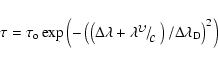 |
(2) |
 |
(3) |
The variables on the left-hand side of the above equation can be
determined from opposite H![]() line wing filtergrams, while
the right-hand side depends on
line wing filtergrams, while
the right-hand side depends on
![]() ,
,
![]() and
and ![]() .
In H
.
In H![]() images of the quiet chromosphere the
fine structures appear on top of a uniform background assumed to have a
zero velocity; moreover they occupy a small percent of the area of the
image. Thus in order to normalize the intensity images and determine the
background intensity we first computed the histogram of the intensity
values over a large area of the quiet chromosphere away from the immediate
vicinity of the sunspot. We further computed the average of the values
contained within 0.67 sigma around the most probable value. We should
note that based on extended experiments Georgakilas (1992)
found that this method gives more accurate results than averaging the
intensity over unstructured regions where one expects the velocity to be
very near zero. In order to compute the line-of-sight velocity from only
two opposite H
images of the quiet chromosphere the
fine structures appear on top of a uniform background assumed to have a
zero velocity; moreover they occupy a small percent of the area of the
image. Thus in order to normalize the intensity images and determine the
background intensity we first computed the histogram of the intensity
values over a large area of the quiet chromosphere away from the immediate
vicinity of the sunspot. We further computed the average of the values
contained within 0.67 sigma around the most probable value. We should
note that based on extended experiments Georgakilas (1992)
found that this method gives more accurate results than averaging the
intensity over unstructured regions where one expects the velocity to be
very near zero. In order to compute the line-of-sight velocity from only
two opposite H![]() wing filtergrams, estimations of the optical depth
at line center and the Doppler width are further needed (see Georgakilas et al. 1990). Bray and others authors successfully
applied the method for studying the physical properties of various
chromospheric features (Bray 1973a,1974; Georgakilas et al. 1990; Suematsu et al. 1995; Malherbe et al. 1997; Georgakilas et al. 2001). We applied the above method in order to compute
line-of-sight velocities from the H
wing filtergrams, estimations of the optical depth
at line center and the Doppler width are further needed (see Georgakilas et al. 1990). Bray and others authors successfully
applied the method for studying the physical properties of various
chromospheric features (Bray 1973a,1974; Georgakilas et al. 1990; Suematsu et al. 1995; Malherbe et al. 1997; Georgakilas et al. 2001). We applied the above method in order to compute
line-of-sight velocities from the H
![]() Å,
H
Å,
H
![]() Å and H
Å and H
![]() Å filtergrams.
We used
Å filtergrams.
We used
![]() and
and
![]() for the optical
depth at line center and Doppler width respectively,
which are the average values for fibrils obtained by
Alissandrakis et al. (1990) with the application
of the cloud model to spectral observations. Estimation of
deviations from these values can be computed from Fig. 2 of
Georgakilas et al. (1990). We further rejected a few points where
the application of the cloud model was not meaningful
(see Georgakilas et al. 1990; Georgakilas 1992).
Since the cloud model is obviously not applicable in the umbra, we
computed the velocities there, assuming a pure Doppler shift model.
We do not consider the velocities computed in this way as accurate
absolute values, but as reliable first order approximations
(see also comments made by Maltby 1975).
for the optical
depth at line center and Doppler width respectively,
which are the average values for fibrils obtained by
Alissandrakis et al. (1990) with the application
of the cloud model to spectral observations. Estimation of
deviations from these values can be computed from Fig. 2 of
Georgakilas et al. (1990). We further rejected a few points where
the application of the cloud model was not meaningful
(see Georgakilas et al. 1990; Georgakilas 1992).
Since the cloud model is obviously not applicable in the umbra, we
computed the velocities there, assuming a pure Doppler shift model.
We do not consider the velocities computed in this way as accurate
absolute values, but as reliable first order approximations
(see also comments made by Maltby 1975).
Following a method based on equations first published by
Kinman (1953) and Plaskett (1952)
and assuming an axial symmetry of the sunspot and of the velocity field
and that the line is formed at the same height over the entire region,
we computed the components of the flow velocity vector as a function of
distance from the center of the spot. We define a coordinate system
centered at the spot with the Z axis along the vertical and the
line-of-sight on the XZ plane with the X axis towards the limb
(see Fig. 1 of Dialetis et al. 1985). We further define u, ![]() ,
and w to be the radial (positive inwards), the
azimuthal (positive in the clockwise direction) and the vertical
(positive upwards) component of the velocity at a point with
coordinates r, and
,
and w to be the radial (positive inwards), the
azimuthal (positive in the clockwise direction) and the vertical
(positive upwards) component of the velocity at a point with
coordinates r, and ![]() on the XY plane. Then the projection
of the velocity on the line-of-sight is given by the equation:
on the XY plane. Then the projection
of the velocity on the line-of-sight is given by the equation:
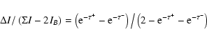
| (4) |
Figure 1 shows images of the sunspot in H![]() center image (a),
and line-of-sight Doppler velocity maps in H
center image (a),
and line-of-sight Doppler velocity maps in H
![]() Å (b), H
Å (b), H
![]() Å (c), and
H
Å (c), and
H
![]() Å (d). The almost circular shape of our
spot and the large scale line-of-sight velocity field reasonably
satisfy the axial symmetry hypothesis (see Dialetis et al. 1985, for criteria). In Fig. 2 we show an azimuthal slice of the
H
Å (d). The almost circular shape of our
spot and the large scale line-of-sight velocity field reasonably
satisfy the axial symmetry hypothesis (see Dialetis et al. 1985, for criteria). In Fig. 2 we show an azimuthal slice of the
H
![]() Å line-of-sight velocity map, measured near
the penumbra-superpenumbra boundary. The solid line corresponds to the
line-of-sight velocity computed from the fitted flow velocity components.
Å line-of-sight velocity map, measured near
the penumbra-superpenumbra boundary. The solid line corresponds to the
line-of-sight velocity computed from the fitted flow velocity components.
In this section we discuss the morphology of the line-of-sight
velocity maps in the three chromospheric layers (defined by
H
![]() Å, H
Å, H
![]() Å, and
H
Å, and
H
![]() Å). We further examine the general characteristics
of the average flow velocity components of the inverse Evershed flow and
compare how they change in the three layers. The results are similar for
all the images we processed. Although we cannot give an exact height
formation of the different H
Å). We further examine the general characteristics
of the average flow velocity components of the inverse Evershed flow and
compare how they change in the three layers. The results are similar for
all the images we processed. Although we cannot give an exact height
formation of the different H![]() wavelengths, measurements at larger
wavelengths, measurements at larger
![]() values correspond to lower chromospheric heights.
For a hydrostatic homogeneous atmospheric model, H
values correspond to lower chromospheric heights.
For a hydrostatic homogeneous atmospheric model, H![]() center is
formed near the 2 Mm height over several hundreds of km. The intensities
in the wings will come from deeper layers; the line wing at
center is
formed near the 2 Mm height over several hundreds of km. The intensities
in the wings will come from deeper layers; the line wing at ![]() 0.35 Å is still close to the layers producing the center of the line,
0.35 Å is still close to the layers producing the center of the line, ![]() 0.5 Å is coming from significantly deeper layers near 1.3 Mm and finally the
line wing at
0.5 Å is coming from significantly deeper layers near 1.3 Mm and finally the
line wing at ![]() 0.75 Å is formed in very deep layers. However the
high chromosphere is inhomogeneous and contributions that form the line
profile probably come from more extended layers.
0.75 Å is formed in very deep layers. However the
high chromosphere is inhomogeneous and contributions that form the line
profile probably come from more extended layers.
From Fig. 1 we observe that there is a close similarity
between the chromospheric velocity maps in H
![]() Å and
in H
Å and
in H
![]() Å, in particular for the more prominent features.
The velocity pattern is slightly more visible in H
Å, in particular for the more prominent features.
The velocity pattern is slightly more visible in H
![]() Å and the absolute values of the velocity are systematically higher
than in H
Å and the absolute values of the velocity are systematically higher
than in H
![]() Å.
At H
Å.
At H
![]() Å the apparent length of the flow channels
is shorter than in H
Å the apparent length of the flow channels
is shorter than in H
![]() Å and in H
Å and in H
![]() Å,
but we do not observe any reversals in the line-of-sight velocities.
In some cases we observe velocity "channels'' that have length similar
to that in H
Å,
but we do not observe any reversals in the line-of-sight velocities.
In some cases we observe velocity "channels'' that have length similar
to that in H
![]() Å, indicating flow velocities that deviate
from the average (we have marked one such channel with a white arrow, in
the upper right part of Fig. 1d).
Å, indicating flow velocities that deviate
from the average (we have marked one such channel with a white arrow, in
the upper right part of Fig. 1d).
In Fig. 3 we compare the line-of-sight velocities related to
the three atmospheric layers for the area of the superpenumbra. It
is verified that the velocity decreases as we move to lower atmospheric
layers, i.e. towards the wings of H![]() .
The scatter plots (Fig. 3)
indicate that the velocities computed at
.
The scatter plots (Fig. 3)
indicate that the velocities computed at
![]() Å are 1.6 times higher than the ones computed at
Å are 1.6 times higher than the ones computed at
![]() Å.
The velocities computed at
Å.
The velocities computed at
![]() Å are about 5.5
times higher than the ones computed at
Å are about 5.5
times higher than the ones computed at
![]() Å.
Finally, the velocities computed at
Å.
Finally, the velocities computed at
![]() Å are
about 9 times higher than the ones computed at
Å are
about 9 times higher than the ones computed at
![]() Å.
The velocity values at
Å.
The velocity values at
![]() Å are of the same
order as in the photosphere but reversed.
Å are of the same
order as in the photosphere but reversed.
In Fig. 4a we present the average flow velocity components for
H
![]() Å. The velocity vector was reconstructed using
the method presented in the previous section. Further Figs. 4b,c
present the average velocity components for H
Å. The velocity vector was reconstructed using
the method presented in the previous section. Further Figs. 4b,c
present the average velocity components for H
![]() Å
and H
Å
and H
![]() Å. We observe that in all three chromospheric
layers the dominant component of the velocity field is the radial and
there is a significant vertical component. The azimuthal component of
the velocity does not show a consistent behavior in the three
chromospheric layers.
Å. We observe that in all three chromospheric
layers the dominant component of the velocity field is the radial and
there is a significant vertical component. The azimuthal component of
the velocity does not show a consistent behavior in the three
chromospheric layers.
The magnitude of the radial and the vertical components for
![]() Å show a maximum value just outside
the penumbral rim. Our results are consistent with that of
Haugen (1969), who found that the vertical velocity
component shows a sharp maximum just outside the penumbral rim.
In Figs. 5a,b we compare the radial and the vertical components
of the flow velocity in the three atmospheric layers. We observe that
the absolute value of the velocity components gradually decrease as we
move lower. We further observe that the maximum of the magnitude of the
velocity shifts towards the inner penumbral boundary as we move at lower
heights within the formation layer of the H
Å show a maximum value just outside
the penumbral rim. Our results are consistent with that of
Haugen (1969), who found that the vertical velocity
component shows a sharp maximum just outside the penumbral rim.
In Figs. 5a,b we compare the radial and the vertical components
of the flow velocity in the three atmospheric layers. We observe that
the absolute value of the velocity components gradually decrease as we
move lower. We further observe that the maximum of the magnitude of the
velocity shifts towards the inner penumbral boundary as we move at lower
heights within the formation layer of the H![]() line. The maximum of
the magnitude is almost at the penumbral rim for
line. The maximum of
the magnitude is almost at the penumbral rim for
![]() Å and just inside the penumbral rim for
Å and just inside the penumbral rim for
![]() Å.
Å.
Using the computed values of the components of the velocity vector of
the inverse Evershed flow, it is possible to obtain information about
the angle ![]() between the velocity vector and the horizontal plane.
More specific
between the velocity vector and the horizontal plane.
More specific ![]() can be determined from the values of the vertical
(w) and the horizontal components of the velocity (u,
can be determined from the values of the vertical
(w) and the horizontal components of the velocity (u,![]() ),
through the relation:
),
through the relation:
![]() .
In Fig. 6 we compare the magnitude of the flow velocity at
H
.
In Fig. 6 we compare the magnitude of the flow velocity at
H
![]() Å (solid line), with angle
Å (solid line), with angle ![]() (dotted line). From the values of angle
(dotted line). From the values of angle ![]() it is clear that the
flow loops are relative flat and probably a fraction, of the ascending
part of the loops, is beyond the velocity field we reconstructed. Our
results indicate that the maximum of the flow velocity coincides with
the region of almost maximum angle between the flow vector and the
horizontal plane and thus with the downstream part of the loop.
Similar results were found by Dialetis et al. (1985); careful
examination of their Figs. 5 and 6 show that for the chromospheric
Evershed flow the maximum of the velocity flow coincides with the
region of almost maximum angle between the flow vector and the
horizontal plane. Also Haugen (1969) found that the
vertical velocity component shows a sharp maximum at the same place
where the inclination of the average velocity vectors with respect
to the horizontal takes its maximum value.
it is clear that the
flow loops are relative flat and probably a fraction, of the ascending
part of the loops, is beyond the velocity field we reconstructed. Our
results indicate that the maximum of the flow velocity coincides with
the region of almost maximum angle between the flow vector and the
horizontal plane and thus with the downstream part of the loop.
Similar results were found by Dialetis et al. (1985); careful
examination of their Figs. 5 and 6 show that for the chromospheric
Evershed flow the maximum of the velocity flow coincides with the
region of almost maximum angle between the flow vector and the
horizontal plane. Also Haugen (1969) found that the
vertical velocity component shows a sharp maximum at the same place
where the inclination of the average velocity vectors with respect
to the horizontal takes its maximum value.
Important conclusions about the nature of the flow can be derived comparing the magnitude of the flow velocity with the angle between the flow vector and the horizontal plane. If the velocity remains subsonic along the loop, then a symmetric flow around the apex of the loop is expected. The flow speed will increase in the upstream part of the loop, attain a maximum value near the region where the flow is horizontal and decrease in the downstream part of the loop (see Figs. 3a and 5a of Thomas 1988). The other possibility is an asymmetric flow with a smooth transition from subsonic to supersonic at the top of the arch. In that case the flow continues to accelerate in the downstream part of the loop, up to a point where it passes from supersonic to subsonic through a compression shock (see Figs. 3c and 5a of Thomas 1988). As we saw from Fig. 6 the flow velocity attains its maximum value at some point in the downstream part of the loop, near the region where the flow shows maximum inclination. This is consistent with a critical flow that attains sonic velocity near the top of the loop and continues to accelerate up to a point in the downstream part of the loop.
Maltby (1975) further suggested that the chromospheric Evershed channels coincide most frequently to dark fibrils. From Fig. 7 we observe that the channels where the residual velocity deviates significantly from the average flow velocity, coincide with dark fibrils. As, due to perspective effects, the sign of the line-of-sight velocity varies around the sunspot, the deviations can be either due to higher than the average absolute velocity values (stronger flow), or due to lower absolute velocity values (weaker flow) along the dark fibrils. Comparison of the residual line-of-sight velocity maps (Figs. 7b,d) with the original line-of-sight velocity maps (Figs. 1b,c), show that the residual velocities along locations corresponding to dark fibrils have the same sign with the original line-of-sight velocities. Thus the velocity deviations related to dark fibrils are due to higher than the average absolute velocity values along these fibrils.
In order to quantitatively verify the relation of higher deviations with
dark fibrils, we computed scatter plots of the residual line-of-sight
velocity maps versus the intensity (sum of opposite wings) (Fig. 8).
The results verify the indication of the visual inspection, since the
deviation from zero increases towards lower intensities. For a limited
number of pixels and for low intensities the residual line-of-sight
velocities appear to deviate significantly from zero; these pixels are
related with a number of dark fibrils. For the vast majority of pixels
the deviation is less than 5 km s-1 at
![]() Å and less than 4 km s-1 at
Å and less than 4 km s-1 at
![]() Å. Taking into
consideration that the deviation is referred to line of sight velocities,
one can plausibly assume that the azimuthally averaged flow velocity is
representative for the majority of flow channels.
Å. Taking into
consideration that the deviation is referred to line of sight velocities,
one can plausibly assume that the azimuthally averaged flow velocity is
representative for the majority of flow channels.
The results of the previous section indicate different properties of the Evershed flow in bright and dark fibrils. Taking advantage of the fact that the method we used for the computation of the components of the flow velocity allows to reject localized flows, we computed the vector of the average flow for mainly bright or dark fibrils alternatively. In order to do that we produced segmented line-of-sight velocity maps in which we have rejected the pixels that correspond to the dark or bright fibrils and then computed the components of the flow velocity based on these images. We should note that we haven't split the images in two segments one with bright fibrils and the other with the remaining fibrils considered dark, but based on the original image we rejected the pixels corresponding to prominent bright or dark fibrils. Thus, each segment contains a number of fibrils that cannot be considered that belong to the one or the other category.
We computed the segmented images from the sum of opposite wing images for each atmospheric level using the "à trous" wavelet transform, a discrete approach to the classical continuous wavelet transform (Starck & Murtagh 1994; Starck et al. 1998). In order to implement the transform the input signal is analyzed by convolving it with a properly chosen low-pass filter, and without following a decimation step. The application of this algorithm on an image results in a set of wavelet coefficients at each level of decomposition, also called wavelet plane, that consists of the same number of pixels as the original image.
Considering a 1D set of sampled data,
![]() ,
then the smoothed data ci (k) at a given resolution i and at
a position k can be obtained by the convolution:
,
then the smoothed data ci (k) at a given resolution i and at
a position k can be obtained by the convolution:
![]() ,
where h is the low-pass filter. The difference between two
consecutive resolution levels:
wi (k) = ci - 1 (k) - ci (k),
represents the wavelet transform of the data at the i level
(Starck & Murtagh 1994). The above algorithm can be easily extended
to 2D space assuming separability which leads to a row-by-row convolution,
followed by column by column convolution. Then from the original image
A0 (x,y) and after the convolution we get a smoothed approximation
A1 (x,y). The first wavelet plane W1 (x,y) is computed by the
difference of the two images. Repeating the above procedure recursively
for every smoothed approximation image for J times and computing the
wavelet planes as the differences between two consecutive approximations
we get at the final level J a set of J+1 images,
W = W1, W2, ...,WJ, AJ. In our implementation we have chosen
a B-spline of degree 3 as scaling function and 5 decomposition levels;
the first plane contains the highest spatial frequencies and the last
the lowest ones.
,
where h is the low-pass filter. The difference between two
consecutive resolution levels:
wi (k) = ci - 1 (k) - ci (k),
represents the wavelet transform of the data at the i level
(Starck & Murtagh 1994). The above algorithm can be easily extended
to 2D space assuming separability which leads to a row-by-row convolution,
followed by column by column convolution. Then from the original image
A0 (x,y) and after the convolution we get a smoothed approximation
A1 (x,y). The first wavelet plane W1 (x,y) is computed by the
difference of the two images. Repeating the above procedure recursively
for every smoothed approximation image for J times and computing the
wavelet planes as the differences between two consecutive approximations
we get at the final level J a set of J+1 images,
W = W1, W2, ...,WJ, AJ. In our implementation we have chosen
a B-spline of degree 3 as scaling function and 5 decomposition levels;
the first plane contains the highest spatial frequencies and the last
the lowest ones.
For each image we computed a sharpened one, adding the first three levels of the "à trous" wavelet transform and a smoothed one adding the rest of the levels; we further smoothed the second image applying a boxcar mean filter. Furthermore we subtracted from the sharpened image the smoothed one and computed a binary mask setting pixel values higher (or lower) than an empirically estimated threshold to 0 and the rest to 1 (Fig. 9). Finally, we multiplied the line-of-sight velocity images by these masks producing segmented images, in which pixels corresponding to bright (or dark) fibrils were set to zero and the rest pixels retained their original values.
We studied the chromospheric Evershed flow from
filtergrams obtained at nine wavelengths along the H![]() profile;
in the following we summarize our results.
profile;
in the following we summarize our results.
As it is clear from the introduction there is a discrepancy concerning the velocity values of the Evershed flow as well as if (assuming a siphon flow along a flux tube) the flow is subcritical (remains subsonic along the whole flux tube) or critical (undergoes a smooth transition from subsonic to supersonic at some point near the apex of the loop). We found that the flow velocity related to some of the more dark superpenumbral fibrils is significantly higher than the average chromospheric Evershed flow. This seems to justify the high velocities reported by early observers who concentrated their attention on the more dark fibrils.
Comparison of the intensity with residual line-of-sight velocities (after subtracting the average flow velocity) verifies the above result, showing significant deviations from the average flow for the pixels related to the most dark fibrils. We further found deviations from the average flow that are larger for the dark fibrils. This indicates that the flow velocity is different for various categories of fibrils and probably time dependent. Still the azimuthally averaged flow velocity can be considered representative for the majority of the flow channels. In order to further investigate the properties of the Evershed flow for different categories of fibrils, we computed the average flow vector from segmented line-of-sight velocity maps, excluding bright or dark fibrils alternatively. We found that the radial component of the flow velocity does not show a significant difference concerning the maximum value. However the magnitude of the vertical component of the flow velocity related to dark fibrils is significantly higher than that related to bright fibrils. This indicates that the inclination angle between the velocity vector and the horizontal plane is lower in the bright fibrils and thus that they are more flat than the dark fibrils. It is possible that this is related to different physical conditions in the fibrils.
The average flow velocities we found in both bright and dark fibrils are subsonic. However the profile of the velocities as a function of distance from the spot center, indicates that the maximum of the velocities is located in the region where the flow vector shows almost maximum inclination with respect to the horizontal; thus the flow speed continues to increase in the descending part of the tube. Even if the error in the estimation of the angle between the flow and the horizontal is large, the fact that the maximum of the radial component of the velocity coincides with the maximum of the vertical component indicates that the flow speed attains its maximum value in the descending part of the loop. This is not consistent with a subcritical flow and can be understood in terms of a critical flow (see Figs. 3 and 5 of Thomas 1988). Thus we can conclude that the flow in the majority of fibrils (for which the average flow can be considered a plausible representative) is critical.
Since the values of the average chromospheric Evershed flow that we found are consistent with previous estimations (e.g. Haugen 1969; Dialetis et al. 1985) a question arises, why while the flow velocity profile indicates that the flow is critical, this is not reflected in the velocity values. A possible answer to this question is that the flow is concentrated in thin channels within the limits of the spatial resolution of our observations; thus we practically compute average line-of-sight velocities. The integration over large angles in order to compute the average flow velocity vector results in further underestimating the velocities.
Finally, we found that the inverse Evershed flow velocity decreases systematically at lower chromospheric heights and the maximum of the flow velocity shifts towards the inner penumbral boundary. We note that recently Hirzberger & Kneer (2001) found an antisymmetric behavior for the photospheric Evershed flow; the flow velocity decreases systematically with photospheric height and the maximum of the flow velocity shifts towards the outer penumbral boundary in higher photospheric layers. This behavior is probably related to the geometry of the fibrils assuming that they extend higher up as we move to higher atmospheric layers.
Acknowledgements
We would like to thank Dr. R. N. Smartt, the T.A.C. of NSO/SP and the staff of the Sacramento Peak Observatory, especially the Observers team of the DST, for their warm hospitality and their help with the observations. We also thank the referee, Dr. R. Schlichenmaier, for constructive criticism.
![\begin{figure}
\par\includegraphics[width=17cm,clip]{3078f1.eps}\end{figure}](/articles/aa/full/2003/21/aa3078/img6.gif)
![\begin{figure}
\par\includegraphics[width=7cm,clip]{3078f2.eps}\end{figure}](/articles/aa/full/2003/21/aa3078/img8.gif)
![\begin{figure}
\par\includegraphics[width=6.4cm,clip]{3078f3a.eps}\par\vspace*{3mm}
\includegraphics[width=6.4cm,clip]{3078f3b.eps}\end{figure}](/articles/aa/full/2003/21/aa3078/img9.gif)
![\begin{figure}
\par\includegraphics[width=7.1cm,clip]{3078f4a.eps}\par\vspace*{2...
...}\par\vspace*{2.5mm}
\includegraphics[width=7.1cm,clip]{3078f4c.eps}\end{figure}](/articles/aa/full/2003/21/aa3078/img10.gif)
![\begin{figure}
\par\includegraphics[width=16.4cm,clip]{3078f7.eps}\end{figure}](/articles/aa/full/2003/21/aa3078/img28.gif)
![\begin{figure}
\par\includegraphics[width=8.2cm,clip]{3078f8a.eps}\par\vspace*{3mm}
\includegraphics[width=8.2cm,clip]{3078f8b.eps}\end{figure}](/articles/aa/full/2003/21/aa3078/img32.gif)
![\begin{figure}
\par\includegraphics[width=16.2cm,clip]{3078f9.eps}\end{figure}](/articles/aa/full/2003/21/aa3078/img38.gif)
![\begin{figure}
\par\includegraphics[width=7cm,clip]{3078f10a.eps}\par\vspace*{3mm}
\includegraphics[width=7cm,clip]{3078f10b.eps}\end{figure}](/articles/aa/full/2003/21/aa3078/img41.gif)