A&A 402, 531-539 (2003)
DOI: 10.1051/0004-6361:20030280
D. K. Chakraborty![]() - M. Das
- M. Das
School of Studies in Physics, Pt. Ravishankar Shukla University, Raipur 492 010, India
Received 27 May 2002 / Accepted 18 February 2003
Abstract
A family of triaxial mass models is described, for which the projected surface density can be calculated analytically, and can show ellipticity variations, isophote twists and high-order residuals. These can be compared with observations. These models are flattened versions of the ![]() -model with density
-model with density
![]() and the modified Hubble model with density profile
and the modified Hubble model with density profile
![]() ,
and are constructed by addition of five spherical harmonic terms to the spherical models. The potential of the models can be expressed in a simple form.
,
and are constructed by addition of five spherical harmonic terms to the spherical models. The potential of the models can be expressed in a simple form.
Key words: galaxies: photometry - galaxies: structure
Triaxial mass models of an alternative form are
![]() ,
where
,
where ![]() is density in the usual spherical polar coordinates
is density in the usual spherical polar coordinates
![]() ,
f(r) is a spherical mass distribution (which is usually a widely studied model), g(r) and h(r) are two suitably chosen radial functions,
,
f(r) is a spherical mass distribution (which is usually a widely studied model), g(r) and h(r) are two suitably chosen radial functions,
![]() and
and
![]() are the usual spherical harmonics. These models also exhibit ellipticity variations and isophote twists in their projections (de Zeeuw & Carollo 1996, hereafter ZC96, Chakraborty & Thakur 2000, hereafter CT00). Such triaxial models with f(r) as the spherical
are the usual spherical harmonics. These models also exhibit ellipticity variations and isophote twists in their projections (de Zeeuw & Carollo 1996, hereafter ZC96, Chakraborty & Thakur 2000, hereafter CT00). Such triaxial models with f(r) as the spherical ![]() -models of Dehnen (1993), are presented in ZC96.
Schwarzschild (1979) studied the triaxial model, wherein f(r) is considered as the spherical modified Hubble model, in a numerical form. Later it was cast into an analytical form by de Zeeuw & Merritt (1983). The projected properties of such triaxial Hubble mass models are described in CT00. We shall refer to these models as fgh models.
-models of Dehnen (1993), are presented in ZC96.
Schwarzschild (1979) studied the triaxial model, wherein f(r) is considered as the spherical modified Hubble model, in a numerical form. Later it was cast into an analytical form by de Zeeuw & Merritt (1983). The projected properties of such triaxial Hubble mass models are described in CT00. We shall refer to these models as fgh models.
Although models with ellipticity variations and isophote twists have been discussed, high-order residuals in these models have not been adequately treated. A small value of
![]() % of the shape parameter has been reported in ZC96. Likewise, the isophotes at large radii are shown to be slightly boxy in CT00.
% of the shape parameter has been reported in ZC96. Likewise, the isophotes at large radii are shown to be slightly boxy in CT00.
Rix & White (1990) have discussed a photometric model, in which an exponential disk is embedded in the equatorial plane of an oblate spheroid of constant ellipticity, and have found that the isophotes are pointy. In a sense, the model is a two component model. Contopoulos & Grosbol (1989) have found an orbital family which can lead to pointy isophotes. Thus, the model of Rix & White is by no means an exclusive interpretation of ellipticals with pointy isophotes. Further, Binney & Petrou (1985) have found that an overpopulation of a particular two dimensional subset of tube orbits can yield boxy isophotes.
Therefore, it will be worthwhile to examine density forms in a triaxial mass model which may produce non elliptical isophotes. For this investigation, we consider the fgh models of ZC96 and CT00. The advantage of this approach is that the potential is known explicitly, and that the projected surface density can be calculated easily (and often, analytically). A disadvantage might be that the use of only the lower order spherical harmonic terms generally leads to models that become peanut-shaped. The addition of higher order spherical harmonic terms leads to more nearly ellipsoidal shapes (Schwarzschild 1993), and "refines" the fgh models (ZC96).
Here we extend the studies of fgh models by including higher-order spherical harmonic terms. We find that the models take more nearly ellipsoidal shapes, and further, the isophotes have high-order residuals. Depending upon the viewing directions, the isophotes are either boxy or pointy. Previous studies of the fgh models lack this feature.
It was shown that the intrinsic shapes of triaxial mass models can be estimated by using photometric data (Thakur & Chakraborty 2001). It is necessary to have a larger ensemble of models, before this method may be applied to elliptical galaxies. The present study of nearly ellipsoidal mass models is also a step towards this goal. Further, the profiles of high-order residuals of the models have some specific features. This may be used to select a galaxy which may be suitable for comparison with the models. For example, for the shape determination of elliptical galaxies, Statler (1994) had selected NGC 3379 and called it the "standard'' elliptical galaxy, because, apart from factors like no sign of ripples or other fine structure, NGC 3379 has almost no isophote twist or ellipticity variation. The latter characteristics make NGC 3379 a suitable candidate for comparison with the models used by Statler, which also do not produce any isophote twist and ellipticity variation.
In Sect. 2, we describe the mass models and in Sect. 3, we present the projected properties. Section 4 is devoted to results and a discussion.
| (1) |
 |
(2) |
![$\displaystyle \frac{1}{\sin\theta }\frac{\partial}{\partial\theta }\left(\sin\t...
... \theta}\right)+\left[{l(l+1)}-\frac{m^{2}}{\sin^{2}\theta}\right]P_{l}^{m} = 0$](/articles/aa/full/2003/17/aah3724/img28.gif) |
(4) |
| (6) |
Applying Eqs. (1)-(3), we obtain the associated density
![]() ,
given by
,
given by
It was realized by Schwarzschild (1979) that while the first term in (8) is spherical, the second term containing Y20 shortens the z-axis and lengthens the x and y axes equally. The third term containing Y22 lengthens the x-axis and shortens the y-axis. This gives rise to a triaxial figure with the major axis along the x-coordinate, the median one along the y-coordinate and the minor one along the z-coordinate. The additional, second and third terms in (7) just reverse the above effects, provided
![]() .
We take
.
We take
![]() for the present study.
for the present study.
![\begin{figure}
\par\includegraphics[width =6.8cm,clip]{h3724f1a.ps}\hspace*{0.4cm}
\includegraphics[width =6.8cm,clip]{h3724f1b.ps}
\end{figure}](/articles/aa/full/2003/17/aah3724/img43.gif) |
Figure 1:
Axial ratios of constant- |
We now consider two specific examples of models. We consider an extension of the models in ZC96, according to the scheme proposed above, and refer to these as models A. We consider a potential of the form (5) and take u(r) of the form
 |
(10) |
 |
(11) |
 |
(12) |
 |
(13) |
| f(r) | = | (14) | |
| g(r) | = | ![$\displaystyle \frac{Mb_{1}}{4\pi}\ \frac{\left[4r^{2}+4(6-\gamma)rb_{2}+\gamma
(5-\gamma)b_{2}^{2}\right]}{r^{\gamma}(b_{2}+r)^{6-\gamma}},$](/articles/aa/full/2003/17/aah3724/img54.gif) |
(15) |
| h(r) | = | ![$\displaystyle \frac{Mb_{3}}{4\pi}\ \frac{\left[4r^{2}+4(6-\gamma)rb_{4}+\gamma(5-\gamma)b_{4}^{2}\right]}{r^{\gamma}(b_{4}+r)^{6-\gamma}},$](/articles/aa/full/2003/17/aah3724/img55.gif) |
(16) |
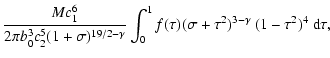
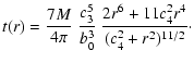
| s(r) | = | ![$\displaystyle \frac{Mc_{1}^{6}}{4\pi b_{0}^{3}}\ \frac{r^{2}\left[8r^{2}+8(10-\gamma)rc_{2}+\gamma(9-\gamma)c_{2}^{2}\right]}{r^{\gamma}(c_{2}+r)^{10-\gamma}}$](/articles/aa/full/2003/17/aah3724/img56.gif) |
(17) |
![$\displaystyle t(r) = \frac{Mc_{3}^{6}}{4\pi b_{0}^{3}}\ \frac{r^{2}\left[8r^{2}...
...)rc_{4}+\gamma(9-\gamma)c_{4}^{2}\right]}{r^{\gamma}(c_{4}+r)^{10-\gamma}}\cdot$](/articles/aa/full/2003/17/aah3724/img57.gif) |
(18) |
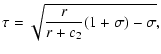
As an another example of triaxial models, we take u(r) to be the potential of the spherical modified Hubble model, defined by the choice
![$\displaystyle u(r)=-\frac{MG}{r}\left\{ln\left[\frac{r}{b_{0}}+\sqrt{1+\frac{r^{2}}{b_{0}^{2}}} \right]\right\} ,$](/articles/aa/full/2003/17/aah3724/img58.gif) |
(19) |
 |
(20) |
 |
(21) |
 |
(22) |
 |
(23) |
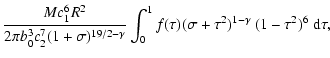
| f(r) | = | (24) | |
| g(r) | = |  |
(25) |
| h(r) | = |  |
(26) |
| s(r) | = | 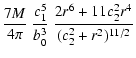 |
(27) |
 |
(28) |
We find that even when
![]() and
and
![]() are considered, the axial ratios of constant-
are considered, the axial ratios of constant-![]() surfaces fall short of p and q, at intermediate radii (see Fig. 1). Confining ourselves to the case where
surfaces fall short of p and q, at intermediate radii (see Fig. 1). Confining ourselves to the case where
![]() and
and
![]() ,
we set the values of
c1,...,c4 such that at a large (finite) and at a small (finite) major axis lengths, the axial ratios of constant-
,
we set the values of
c1,...,c4 such that at a large (finite) and at a small (finite) major axis lengths, the axial ratios of constant-![]() surfaces become close to p and q (Appendix A).
surfaces become close to p and q (Appendix A).
We have adopted a form (7) of density distribution and a procedure to determine c1,...,c4. The resulting density figure is nearly ellipsoidal: serious dimples of the fgh model have almost disappeared (see Fig. 2). The method adopted here is different from that adopted by Schwarzschild (1993), who used a form equivalent to a 10 term development in spherical harmonics.
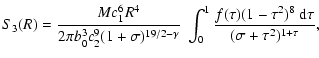
| S1(R) | = |  |
(31) |
| S2(R) | = |  |
(32) |
| S3(R) | = | 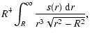 |
(33) |
Although the potential
![]() and the associated density
and the associated density
![]() are the same as in the fgh models studied by earlier workers, we note that
are the same as in the fgh models studied by earlier workers, we note that
![]() is now different from the projected density
is now different from the projected density
![]() of the fgh models. The additional terms with radial functions s(r) and t(r), which are included in the present study, also contribute to
of the fgh models. The additional terms with radial functions s(r) and t(r), which are included in the present study, also contribute to
![]() .
However, the contributions from these additional terms are small compared to those from the terms with radial functions f(r),g(r) and h(r). The functional form of
.
However, the contributions from these additional terms are small compared to those from the terms with radial functions f(r),g(r) and h(r). The functional form of
![]() is same as that of
is same as that of
![]() .
We follow the derivations made in ZC96 and define the position angle
.
We follow the derivations made in ZC96 and define the position angle
![]() of
of
![]() by
by
| (35) |
| (36) |
| (37) |
| |
= | (38) | |
| = | (39) |
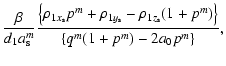
![\begin{figure}
\par\includegraphics[width =8.5cm,clip]{h3724f3.ps}
\end{figure}](/articles/aa/full/2003/17/aah3724/img95.gif) |
Figure 3:
Radial profiles of B4 and A4 for models with p=0.9, q=0.7. Frame a) presents model A with
|
 |
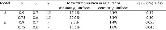
We have obtained the projected density of a family of triaxial mass models which are nearly ellipsoidal. Although the complexity of the problem has led us to some long expressions, the numerical evaluation of these to obtain the projected parameters, in terms of different choices of the model parameters and viewing angles, is straightforward.
Figure 1 shows the axial ratios of constant density surfaces of the models A and B. We find that the axial ratios of constant-![]() surfaces at intermediate radii, vary considerably from their values at asymptotic radii. These variations are relatively small for the constant-
surfaces at intermediate radii, vary considerably from their values at asymptotic radii. These variations are relatively small for the constant-![]() surfaces. For the model A with
p=0.75, q=0.6,
surfaces. For the model A with
p=0.75, q=0.6,
![]() ,
the maximum relative change in the axial ratios of constant-
,
the maximum relative change in the axial ratios of constant-![]() surfaces is
surfaces is ![]() 25.0%, which drops to
25.0%, which drops to ![]() 8.3% for constant-
8.3% for constant-![]() surfaces. For the same choice of p and q, the model B exhibits the maximum relative change in the axial ratios of
surfaces. For the same choice of p and q, the model B exhibits the maximum relative change in the axial ratios of ![]() 11.6% for constant-
11.6% for constant-![]() surfaces and
surfaces and ![]() 1.6% for constant-
1.6% for constant-![]() surfaces. For the rounder models, e.g. with
p=0.9, q=0.7 these variations are relatively small.
surfaces. For the rounder models, e.g. with
p=0.9, q=0.7 these variations are relatively small.
In Fig. 2, we present the sections of constant density surfaces of the models and the ellipsoids, with the same p and q, in the (x-z) plane. While the constant-![]() is dimpled (peanut-shaped), the constant-
is dimpled (peanut-shaped), the constant-![]() is relatively smooth and closer to the ellipsoid.
is relatively smooth and closer to the ellipsoid.
In Sect. 3, we have defined
![]() and
and
![]() ,
which are related to high-order residuals on constant-
,
which are related to high-order residuals on constant-
![]() contours. The surface photometry data of elliptical galaxies are obtained by considering variations around the best-fitting ellipse. In order to compare the model with data, we use the standard routines of ellipse-fitting based on the algorithm of Jedrzejewski (1987), and obtain the parameters of the best-fitting ellipses on
contours. The surface photometry data of elliptical galaxies are obtained by considering variations around the best-fitting ellipse. In order to compare the model with data, we use the standard routines of ellipse-fitting based on the algorithm of Jedrzejewski (1987), and obtain the parameters of the best-fitting ellipses on ![]() and the high-order residuals A3, B3, A4, B4 on the ellipses. We find that B4 is positive when viewed almost along the (x-y) plane and it is negative when viewed at narrow angles with respect to the
and the high-order residuals A3, B3, A4, B4 on the ellipses. We find that B4 is positive when viewed almost along the (x-y) plane and it is negative when viewed at narrow angles with respect to the ![]() directions. At intermediate viewing angles, B4 is partly positive and partly negative. A4 is small compared to B4, and the residuals A3 and B3 are negligible.
directions. At intermediate viewing angles, B4 is partly positive and partly negative. A4 is small compared to B4, and the residuals A3 and B3 are negligible.
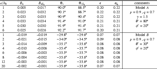
Figure 3 and Table 1 present the radial profiles of B4 and A4 to a radial distance of nearly four times the effective radius of each model. Table 1 also presents the profiles of basic parameters, namely, the position angle
![]() of the major axis and the ellipticity
of the major axis and the ellipticity ![]() of the best-fitting ellipse, and the corresponding parameters
of the best-fitting ellipse, and the corresponding parameters
![]() and
and
![]() of the constant-
of the constant-
![]() contour. It is seen that the basic parameters of the best-fitting ellipses are very close to those of the
constant-
contour. It is seen that the basic parameters of the best-fitting ellipses are very close to those of the
constant-
![]() contours. Finally, we find the centres of the best-fitting ellipses coincide with the centre of
contours. Finally, we find the centres of the best-fitting ellipses coincide with the centre of ![]() .
.
Models A and B appear to be either boxy or pointy, depending upon the viewing direction. Regions of these viewing directions are shown in Fig. 4. We find that the model A exhibits three distinct regions of viewing angles producing boxy (region 1), partly boxy and partly pointy (region 2) and pointy (region 3) isophotes. On the other hand the model B shows regions 1 and 2 only.
To understand this feature, we perform the following numerical experiment. We obtain the residuals on the best-fitting ellipses on
![]() .
The isophotes of
.
The isophotes of
![]() are found to be boxy in all the viewing directions. It follows that the pointy isophotes of
are found to be boxy in all the viewing directions. It follows that the pointy isophotes of ![]() arise only from the s and t terms in
arise only from the s and t terms in ![]() (see Eqs. (B.2) and (B.3)). A measure of the contributions from the s and t terms in
(see Eqs. (B.2) and (B.3)). A measure of the contributions from the s and t terms in ![]() ,
may be the average of the ratio
(s+t)/(g+h). Further, note that the terms s and t were added to reduce the variations in the axial ratios of the fgh models (cf. Fig. 1). Therefore, it is expected that the contributions from the s and t terms should be related to the variations in the axial ratios. Table 1 presents these parameters. It is seen that <
(s+t)/(g+h)> is smaller in model B than in model A. Consistently, the variation in axial ratios in model B is smaller than in model A.
,
may be the average of the ratio
(s+t)/(g+h). Further, note that the terms s and t were added to reduce the variations in the axial ratios of the fgh models (cf. Fig. 1). Therefore, it is expected that the contributions from the s and t terms should be related to the variations in the axial ratios. Table 1 presents these parameters. It is seen that <
(s+t)/(g+h)> is smaller in model B than in model A. Consistently, the variation in axial ratios in model B is smaller than in model A.
The isophotes of elliptical galaxies with disks have been found to exhibit similar behavior (Scorza & Bender 1995; Rix & White 1990). Using a model with an exponential disk embedded in an oblate spheroid, Rix and White have found that B4 is positive, which is the photometric signature of the disk, only when the angle i of the disk from the line of sight is less than
![]() .
In the mass models presented here, the radial functions s(r) and t(r) decay faster than the other radial functions, both at small and at large radii. The terms in
.
In the mass models presented here, the radial functions s(r) and t(r) decay faster than the other radial functions, both at small and at large radii. The terms in ![]() with these radial functions, appear to mimic a disc in projection.
with these radial functions, appear to mimic a disc in projection.
The analytical formulation gives us some insight. We find that the fourth order residuals
![]() and
and
![]() arise, only from the fourth order spherical harmonic terms in
arise, only from the fourth order spherical harmonic terms in ![]() ,
and no third order or higher order residuals are present in our analytical formulation. Our results of the ellipse-fitting algorithm are consistent with these analytical findings. We also note that the projected density has the symmetry
,
and no third order or higher order residuals are present in our analytical formulation. Our results of the ellipse-fitting algorithm are consistent with these analytical findings. We also note that the projected density has the symmetry
![]() .
The radial coordinate of the points on an ellipse, with centre as origin, also has this symmetry. We may anticipate that the centre of the best-fitting ellipse should coincide with the center of
.
The radial coordinate of the points on an ellipse, with centre as origin, also has this symmetry. We may anticipate that the centre of the best-fitting ellipse should coincide with the center of ![]() .
This is found to be true.
.
This is found to be true.
Although,
![]() can not be compared with the observations, it can still be used for a qualitative estimate of the variation in the high-order residual with the viewing direction. Only for the rounder models with
p=0.9, q=0.7,
can not be compared with the observations, it can still be used for a qualitative estimate of the variation in the high-order residual with the viewing direction. Only for the rounder models with
p=0.9, q=0.7,
![]() is close to B4 (see Table 1). However, the ellipticity and position angle of the best-fitting ellipse are quite close to the ellipticity and position angle of
is close to B4 (see Table 1). However, the ellipticity and position angle of the best-fitting ellipse are quite close to the ellipticity and position angle of
![]() ,
for any semi major axis length, even for the flatter models with
p=0.75, q=0.6.
,
for any semi major axis length, even for the flatter models with
p=0.75, q=0.6.
Acknowledgements
DKC, a Visiting Associate of the Inter-University Centre for Astronomy and Astrophysics (IUCAA), Pune, India, and MD express their sincere thanks to IUCAA for providing local hospitality and support during IUCAA visits. Partial support is also provided through the CSIR project grant No. 03(0807)/97/EMR-II, which is gratefully acknowledged. We are very grateful to the anonymous referee for his critical comments and useful suggestions, which helped us to improve the paper enormously.
We expand s(r) and t(r) at large and at small r and retain the terms of highest orders only, in ![]() .
Requiring that at a large and at a small major axis lengths, denoted
.
Requiring that at a large and at a small major axis lengths, denoted ![]() and
and ![]() ,
respectively, axial ratios of constant-
,
respectively, axial ratios of constant-![]() surfaces are same as p and q, we obtain
surfaces are same as p and q, we obtain
| c1n | = | 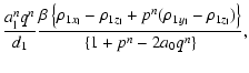 |
(A.1) |
| c3n | = | 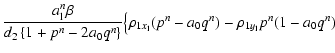 |
|
| (A.2) |
| |
= |  |
(A.3) |
| = | |||
| (A.4) |
Integrating ![]() along the line of sight, we obtain
along the line of sight, we obtain
| |
= | ||
| (B.1) |
| E1 | = | 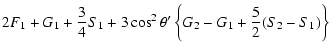 |
|
 |
|||
| (B.2) |
| E2 | = | ||
| E3 | = | ||
| E4 | = | ||
| E5 | = | ||
| E6 | = | ||
| E7 | = | ||
| E8 | = | ||
| E9 | = | (B.3) |
| P0 | = | ||
| P2 | = | ||
| P3 | = | ||
| P4 | = | ||
| P5 | = | (B.4) |
The radial functions S1, S2, S3, T1, T2, T3, H1, H2, G1, G2 and F1 in
P0...P5 can be evaluated analytically. The integrands can be cast as integral powers of
![]() which can be integrated easily. Writting
which can be integrated easily. Writting
| I1 | = | R6t1+3R4t2+3R2t3+t4, | |
| I2 | = | R4t1+2R2t2+t3, | |
| I3 | = | R2t1+t2 |
| I4 = t1, | (C.1) |
we have
| S1(R) | = | ||
| S2(R) | = | 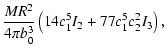 |
|
| S3(R) | = | 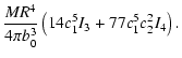 |
(C.2) |
The formulae given in (31)-(33) are not very useful for numerical computations because of the infinite integration intervals and singularities of the integrands. Following Dehnen (1993) and Thakur & Chakraborty (2001), we put
 |
(D.1) |
| |
= | ||
| (D.5) |
Similar forms for integrals F1, G1 and G2 are reported in Thakur & Chakraborty (2001).
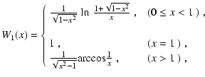
For integer ![]() ,
the integral F1, G1, G2, S1,
S2 and S3 can be written in terms of functions Wn(x), which are
defined as follows (ZC96):
,
the integral F1, G1, G2, S1,
S2 and S3 can be written in terms of functions Wn(x), which are
defined as follows (ZC96):
and
In Table E.1, we present the functions S1, S2 and S3, expressed in terms of Wn(x). Functions F1, G1, G2 in terms of Wn(x) are reported in ZC96.
![\begin{table}
\par
\begin{tabular*}{135mm}%
{@{\extracolsep{\fill}}ll}\hline\hli...
...})+39W_{7}(R/c_{2})+21W_{8}(R/c_{2})]$\space \\ \hline
\end{tabular*}\end{table}](/articles/aa/full/2003/17/aah3724/img158.gif) |
![\begin{figure}
\par\mbox{\includegraphics[width=6.5cm,clip]{h3724f2a.ps}\hspace*{0.5cm}
\includegraphics[width=6.5cm,clip]{h3724f2b.ps} }\end{figure}](/articles/aa/full/2003/17/aah3724/img59.gif)
![\begin{figure}
\par\mbox{\includegraphics[width=6.4cm,clip]{h3724f4a.ps}\hspace*{0.9cm}
\includegraphics[width =6.4cm,clip]{h3724f4b.ps} }\end{figure}](/articles/aa/full/2003/17/aah3724/img98.gif)