We consider now the motions excited by torques of low
frequencies (
![]() ). The potentials responsible for these
torques are of type (n,0). The nutations produced are below our
cut-off level of 0.05
). The potentials responsible for these
torques are of type (n,0). The nutations produced are below our
cut-off level of 0.05 ![]() asamplitude for all n>4.
asamplitude for all n>4.
The Chandler resonance plays a major role in the wobble response to
forcing in this band; so the value of ![]() which appears in the
Chandler frequency assumes significance. The effects of mantle
anelasticity and ocean tides on nutations can be dealt with by taking
into account the complex increments that they produce to the values
of
which appears in the
Chandler frequency assumes significance. The effects of mantle
anelasticity and ocean tides on nutations can be dealt with by taking
into account the complex increments that they produce to the values
of ![]() and other compliances, a fact that was exploited by
Mathews et al. (2002) in their treatment of low frequency nutations
and retrograde diurnal wobbles. In that context, the anelasticity
contribution was practically independent of frequency while the
ocean tide admittances were strongly frequency dependent, not only
due to the FCN resonance, but also because of other aspects of ocean
dynamics. In the low frequency tidal band that we are concerned with
now, the ocean tides are believed to be essentially equibrium tides,
with a constant admittance; but the anelasticity effect varies
strongly with frequency across the band, making the anelasticity
contribution to
and other compliances, a fact that was exploited by
Mathews et al. (2002) in their treatment of low frequency nutations
and retrograde diurnal wobbles. In that context, the anelasticity
contribution was practically independent of frequency while the
ocean tide admittances were strongly frequency dependent, not only
due to the FCN resonance, but also because of other aspects of ocean
dynamics. In the low frequency tidal band that we are concerned with
now, the ocean tides are believed to be essentially equibrium tides,
with a constant admittance; but the anelasticity effect varies
strongly with frequency across the band, making the anelasticity
contribution to ![]() strongly dependent on the forcing
frequency. So the apparent frequency of the Chandler resonance,
strongly dependent on the forcing
frequency. So the apparent frequency of the Chandler resonance,
![]() cpsd, is itself a function of the
excitation frequency
cpsd, is itself a function of the
excitation frequency ![]() .
More precisely, the polar motion
response (37) to forcing at
.
More precisely, the polar motion
response (37) to forcing at ![]() cpsd is as if there is a resonance
at
cpsd is as if there is a resonance
at
![]() .
The Chandler eigenfrequency
.
The Chandler eigenfrequency
![]() (i.e. the frequency of the free Chandler wobble mode) is not
variable, of course. It is given by the value of
(i.e. the frequency of the free Chandler wobble mode) is not
variable, of course. It is given by the value of
![]() for
the specific excitation frequency
for
the specific excitation frequency ![]() at which Re
at which Re
![]() .
Another aspect that cannot be ignored is that the imaginary part
of the anelasticity contribution to
.
Another aspect that cannot be ignored is that the imaginary part
of the anelasticity contribution to ![]() has to be taken with
a sign opposite to that of the forcing frequency: positive for
retrograde wobbles and negative for prograde ones. This is
required for ensuring that the tidal deformation lags behind the
tidal forcing; see Mathews et al. (2002), Appendix C, for
details.
has to be taken with
a sign opposite to that of the forcing frequency: positive for
retrograde wobbles and negative for prograde ones. This is
required for ensuring that the tidal deformation lags behind the
tidal forcing; see Mathews et al. (2002), Appendix C, for
details.
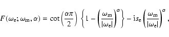
The anelasticity model adopted in this work is the one employed by
Mathews et al. (2002). It belongs to the class of models that
Wahr & Bergen (1986)
refer to as the ![]() model of
Sailor & Dziewonski
(1978). The essential feature of these models is that the value of a
deformational response parameter (e.g.,
model of
Sailor & Dziewonski
(1978). The essential feature of these models is that the value of a
deformational response parameter (e.g., ![]() )
of the anelastic
Earth to harmonic excitation at some frequency
)
of the anelastic
Earth to harmonic excitation at some frequency
![]() differs from the
elastic-Earth value at a reference frequency
differs from the
elastic-Earth value at a reference frequency
![]() by an amount
proportional to
by an amount
proportional to
 |
(39) |
It is evident, however, that the model (39) cannot remain valid
down to zero frequency: F would become infinite at ![]() ,
leading to
an infinite anelasticity contribution. The zero frequency term
present in the (4, 0) tidal potential presents, therefore, an
exception that cannot be handled by the above procedure. The
deformational responses to an incessantly acting potential
should actually be characterized by the so-called secular or
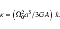
fluid Love numbers. Now, the compliance
,
leading to
an infinite anelasticity contribution. The zero frequency term
present in the (4, 0) tidal potential presents, therefore, an
exception that cannot be handled by the above procedure. The
deformational responses to an incessantly acting potential
should actually be characterized by the so-called secular or
fluid Love numbers. Now, the compliance ![]() is known to have
a simple relation to the k Love number (see, for example,
Sasao et al. 1980):
is known to have
a simple relation to the k Love number (see, for example,
Sasao et al. 1980):
 |
(40a) |
 |
(40b) |
This finding has interesting consequences. One sees trivially that
with ![]() and
and
![]() ,
the frequency domain Eqs. (32) lead to the unphysical result that
,
the frequency domain Eqs. (32) lead to the unphysical result that
![]() is infinite.
One has to go back therefore to the time domain Eqs. (29),
with
is infinite.
One has to go back therefore to the time domain Eqs. (29),
with
![]() and
and
![]() replaced by the expressions (31), noting
that the
replaced by the expressions (31), noting
that the
![]() terms drop out since m=0 the present case.
One sees
immediately that the terms proportional to
terms drop out since m=0 the present case.
One sees
immediately that the terms proportional to
![]() in Eq. (29a)
cancel out as a consequence of the vanishing of
in Eq. (29a)
cancel out as a consequence of the vanishing of ![]() ,
and that
in the entirely adequate approximation wherein terms of
,
and that
in the entirely adequate approximation wherein terms of
![]() are neglected, the two equations then take the forms
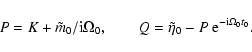
are neglected, the two equations then take the forms
![]() and
and
![]() ,
with
,
with
![]() .
Subtraction of one from the other yields
.
Subtraction of one from the other yields
![]() ,
which is a constant in the present case since
,
which is a constant in the present case since
![]() is.
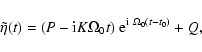
The solution for
is.
The solution for
![]() is then immediate:
is then immediate:
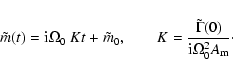 |
(41) |
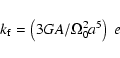
The initial value
![]() of
of
![]() is arbitrary. The value of K in
the case of the (4, 0) potential may be obtained from Eqs. (28) and (27):
is arbitrary. The value of K in
the case of the (4, 0) potential may be obtained from Eqs. (28) and (27):
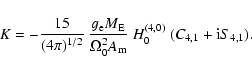 |
(42) |
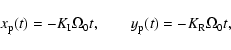
The solution (41) describes a secular motion, relative to the pole of
maximum moment of inertia, of the Earth's instantaneous rotation pole.
The associated nutation
![]() ,
obtained by integrating
Eq. (11) after introducing (41), is
,
obtained by integrating
Eq. (11) after introducing (41), is
 |
(43) |
 |
(44) |
| (45) |
 |
(46) |
Copyright ESO 2003