2 Wobble, nutation, and polar motion: Kinematics

2.1 Wobbles

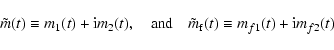
The wobbles of the mantle and the fluid core are described by  ${\vec m}(t)$ and  ${\vec m}_{\rm f}(t)$, defined in terms of the instantaneous angular velocity vectors ${\vec \Omega}, {\vec \Omega}_{\rm f}$ of the respective regions by

$${\vec \Omega}\!=\!\Omega_0~\left[(1+m_3)~{\vec i}_3+ {\vec m}... ...!\Omega_0~\left[m_{f3}~ {\vec i}_3+{\vec m}_{\rm f}(t)\right],$$ (1)

where ${\vec i}_3$ is the axis of maximum moment of inertia of the Earth, $\Omega_0$ is mean angular velocity of Earth rotation, equivalent to 1 cpsd, and m₃ and (m₃+m_f3) represent the fractional variations in the axial spin rates of the mantle and the core, respectively. As is well known, use of the complex combinations

$$\tilde m(t)\equiv m_1(t)+{\rm i}m_2(t), \quad{\rm and}\quad \tilde m_{\rm f}(t)\equiv m_{f1}(t)+{\rm i}m_{f2}(t)$$ (2)

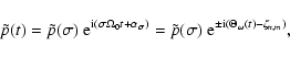
of the components of ${\vec m}(t)$ and ${\vec m}_{\rm f}(t)$ helps to express the dynamical equations of the wobbles compactly. Their individual spectral components have the forms

$$\tilde m(t)= \tilde m(\sigma)\ {\rm e}^{{\rm i}(\sigma\Omega_... ... f}(\sigma)\ {\rm e}^{{\rm i}(\sigma\Omega_0t+\alpha_\sigma)},$$ (3)

where $\sigma$ is the frequency (in cpsd) and  $\alpha_\sigma$ is the phase, of the wobble; $\sigma$ is positive (negative) for prograde (retrograde) wobbles.

The phase of a wobble due to lunisolar forcing is related, of course, to the argument of the relevant spectral component of the lunisolar potential. In the convention of Cartwright & Tayler (1971), the potential of spherical harmonic type (n,m) and frequency $\omega$ at the point with colatitude $\theta$ and longitude $\lambda$ at a geocentric distance r is expressed as

$$V_{\omega}^{(n,m)}({\vec r};t) = g_{\rm e} H^{(n,m)}_\omega~(... ...a,\lambda)~ {\rm e}^{{\rm i}(\Theta_\omega(t)-\zeta_{n,m})}~],$$ (4)

where $a_{\rm e}$ is the Earth's equatorial radius, $g_{\rm e}=GM_{\rm E}/a_{\rm e}^2$ ($M_{\rm E}$ being the Earth's mass), and $H^{(n,m)}_\omega$ is the amplitude (expressed as a height) and  $\Theta_\omega(t)$ is the argument of this spectral component of the tidal potential. The role of $\zeta_{n,m}$, defined by

$$\zeta_{n,m} 0 \quad {\rm for}\ (n-m)\ {\rm even} \quad {\rm and}$$ =

$$\zeta_{n,m} \pi/2 \quad {\rm for}\ (n-m)\ {\rm odd},$$ = (5)

is to ensure that the potential involves $\cos\Theta_\omega(t)$ or $\sin\Theta_\omega(t)$ according as (n-m) is even or odd, in conformity with the Cartwright-Tayler convention. The argument  $\Theta_\omega(t)$ is expressed as a linear combination, with integer coeffients, of the Doodson's fundamental tidal arguments $(\tau-\lambda, s, h, p, N', p_s)$, with m as the coefficient of the first of these. It is useful to note that $\tau+s-\lambda= GMST+\pi$, GMST being the Greenwich Mean Sidereal Time (in radians). For all practical purposes, $\Theta_\omega(t)$ is a linear function of time, and

$$\omega= {{\rm d} \Theta_\omega(t)\over {\rm d}t},$$ (6)

with $\omega$ confined, for given m, to the interval

$$0\le \omega< (1/2)~\Omega_0,\quad (m=0); \quad {\rm and}$$

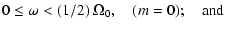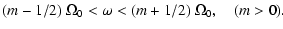$$(m-1/2)~\Omega_0<\omega<(m+1/2)~\Omega_0, \quad (m>0).$$ (7)

The torque exerted by the potential (4) on the Earth, which is considered in detail in the next section, has both prograde and retrograde components. The relation between the argument $\Theta_\omega(t)$ and the phases $(\sigma\Omega_0t+\alpha_\sigma)$ of the wobbles produced by the respective components of the torque is

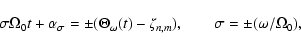$$\sigma\Omega_0t+\alpha_\sigma= \pm (\Theta_\omega(t)-\zeta_{n,m}), \qquad \sigma=\pm(\omega/\Omega_0),$$ (8)

wherein the upper (lower) signs are for the prograde (retrograde) wobbles. As we shall show in Sect. 6, an unusual situation arises in the case of the nonrigid Earth if the driving torque is time independent ($\sigma=0$): the solution is then not a special case of (3), but is linear in t:

$$\tilde m(t)={\rm i}\Omega_0~Kt+K'.$$ (9)

2.2 Nutations

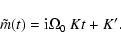
The complex nutation variable $\tilde\eta(t)$, defined by

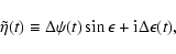$$\tilde\eta(t)\equiv \Delta\psi(t)\sin\epsilon+ {\rm i}\Delta\epsilon(t),$$ (10)

is kinematically related to the mantle wobble variable $\tilde m(t)$:

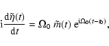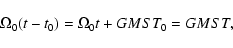
$${\rm i}{{\rm d}\tilde\eta(t)\over {\rm d}t} = \Omega_0~\tilde m(t)~{\rm e}^{{\rm i}\Omega_0(t-t_0)} ,$$ (11)

where -t₀ (or $-\Omega_0t_0$ in angle units) is GMST₀, the Greenwich Mean Sidereal Time (GMST) at the epoch chosen as the origin of time (t=0). It is conventional, in both tidal and nutation theories, to take this epoch to be J2000, i.e., 12 hrs UT1 on January 1, 2000, and we follow this convention.

$$\Omega_0(t-t_0) = \Omega_0t+GMST_0 = GMST,$$ (12)

where GMST₀=4.894961212 radians.

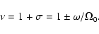
Equation (11) is a linear approximation to the exact relation, and is entirely adequate for the present purposes. Taken together with Eqs. (3) and (12), it implies that a wobble of frequency $\sigma$ cpsd ( $\sigma\ne -1$ or 0) has the associated nutation of frequency $\nu$ cpsd:

$$\tilde\eta(t) -{\tilde m(\sigma)\over 1+\sigma}\ {\rm e}^{{\rm i}[~\nu\Omega_0t+\alpha_\sigma+ GMST_0~]}$$ =

$$-{\tilde m(\sigma)\over 1+\sigma}\ {\rm e}^{{\rm\pm i}(\Theta_\omega(t)- \zeta_{n,m})+{\rm i} GMST},$$ = (13)

where, in view of the second of Eqs. (8),

$$\nu=1+\sigma=1\pm \omega/\Omega_0.$$ (14)

The plus (minus) sign in the above equation is for prograde (retrograde) wobbles.

Now, the conventional argument $\Xi_\nu$ of a nutation of frequency $\nu$ is related to the argument $\Theta_\omega(t)$ of the tide which excites the nutation through

$$\Xi_\nu =\pm(\Theta_\omega(t)-m\pi)+GMST,$$ (15a)

$${\rm e}^{{\rm i}\Xi_\nu}= (-1)^m~{\rm e}^{{\rm\pm i}\Theta_\omega(t)+{\rm i} GMST}.$$ (15b)

Therefore the expression (13) for $\tilde\eta(t)$ becomes, for a nutation excited by a tidal potential of order m,

$$\tilde\eta(t) (-1)^m \tilde\eta(\nu){\rm e}^{{\rm i}\Xi_\nu(t)\mp {\rm i}\zeta_{n,m}},$$ = (16)

$$\tilde\eta(\nu) {-\tilde m(\sigma)\over 1+\sigma}\cdot$$ = (17)

The relations (15) give rise to the factor (-1)^m which appears in (16). This factor which would have been missed if the constants in the phases of the wobbles and nutations were not explicitly kept track of, and the factor e $^{{\rm\mp i}\zeta_{n,m}}$ (which is 1 or $\rm\mp i$ according as n-m is even or odd), play essential roles in correctly identifying the coefficients of  $\cos\Xi_\nu(t)$ and  $\sin\Xi_\nu(t)$ computed from the tidal potential, and in ensuring that they have the correct signs.

The special case $\sigma= -1$ leads to a secularly varying $\tilde\eta(t)$, representing precession:

$$\tilde\eta(t)= \tilde m(-1)~{\rm i}\Omega_0t+\tilde\eta(0).$$ (18)

2.3 Polar motion

Polar motion is represented by

$$\tilde p(t)\equiv x_{\rm p}(t)-{\rm i}y_{\rm p}(t)=-\tilde\eta(t){\rm e}^{{\rm -i} GMST},$$ (19)

as has been made explicit by Gross (1992) and Brzezinski & Capitaine (1993). It is evident that its frequency is $(\nu-1)=\sigma$ cpsd, i.e., the same as that of the associated wobble. One obtains, on using (13),

$$\tilde p(t)= \tilde p(\sigma) ~{\rm e}^{{\rm i}(\sigma\Omega_... ... p(\sigma)~{\rm e}^{{\rm\pm i}(\Theta_\omega(t)-\zeta_{n,m})},$$ (20)

$$\tilde p(\sigma) = {\tilde m(\sigma)\over(1+\sigma)}\cdot$$ (21)

In the special case when the torque is time independent ($\sigma=0$), one finds on integrating Eq. (11) with  $\tilde m(t)$ taken from (9), and then using (19), that

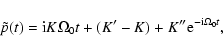$$\tilde p(t)= {\rm i}K\Omega_0t+(K'-K)+K'' {\rm e}^{{\rm -i}\Omega_0t},$$ (22a)

where K' and K'' involve the intial values of $\tilde m$ and $\tilde p$. The specifics of this case are dealt with in Sect. 6. The nutation corresponding to (22a) is

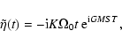$$\tilde\eta(t) = -{\rm i}K\Omega_0t~ {\rm e}^{{\rm i}GMST},$$ (22b)

with the omission of the initial value terms. A nutation of this type, which is periodic but with an amplitude varying linearly with time, appears to have been not encountered before.