5 Clustering properties of bright lumps: Cluster dimensions on scales of a few 100 pc

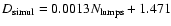
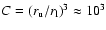
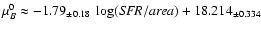
Figure 7: Left: cumulative number vs. aperture radius for the detected lumps within selected galaxies. Logarithms are given to base $\sqrt {2}$. The slope of the straight parts gives the cluster dimension. Fat lines represent large-scale length (and high-lump number) galaxies, thin lines short-scale length (and low-lump number) galaxies. Right: reduced bright-lump cluster dimension vs. extrapolated central surface brightness. The symbol size indicates the number of lumps used for the determination of the observed (non-reduced) cluster dimension. The line corresponds to a bisector fit to the data (equation given in the text).

Star-forming complexes in dwarf galaxies form non-random point patterns also in a sense different from that discussed in Sect. 4.3. Their positions correlate according to a self-similar (fractal) arrangement. In this section we substantiate this claim studying an index devoted to spatial statistics, namely the correlation or clustering dimension, as applied to two-dimensional bright-lump distributions.

As observed by Elmegreen & Elmegreen (2001), the distribution of bright-lump center positions on a kiloparsec scale in spiral and irregular galaxies obey a power-law behaviour similar to the fractal structure of the interstellar gas with fractal dimension D₃=2.3. Thus the center positions of star-forming aggregates within isolated areas of large galaxies are fractal. Here we address the question whether star-forming complexes that are scattered over the entire disks of dwarf galaxies are non-randomly distributed as well. We restrict our inquiry to the dwarfs of our sample that exhibit more than 20 bright lumps. Given our photometry with image scales of typically well above 10 parsecs/pixel and seeing conditions of a few pixels we expect to only dissolve structures larger than about 100 parsecs. Thus small-scale clustering and the accompagning blending effects (Elmegreen & Elmegreen 2001) are of no concern to our study. To quantify the spatial clustering of the position patterns we adopt the cumulative distance method (Hastings & Sugihara 1996): a power law relationship $N(r) \propto r^D$ is assumed for the cumulative number of points N(r) within a distance r around each point. If the distribution is (at least partially) self-similar this will be manifested in a $\log(N)$-$\log(r)$ diagram as a straight line with slope D, called the cluster (or correlation) dimension,

$$D= \frac{{\rm d}~\log N(r)}{{\rm d}~\log r}\cdot$$

The more highly clustered the points (at all relevant scales), the lower the cluster dimension. For a random or Poissonian distribution of points on a two-dimensional plane one has $D\approx2$, independent of the number of points involved, which only governs the error estimate. The graphs for six observed galaxies with 20-30 lumps and for five galaxies with about 200-300 lumps are shown in Fig. 7, left, plotted with thin and thick lines, respectively. For both groups the relevant scaling range, i.e. the straight part of the curve, lies between about 100 ($\approx$ $\sqrt{2}^{13}$) and 1000 ($\approx$ $\sqrt{2}^{20}$) parsecs. The galaxies with lower lump numbers exhibit smaller cluster dimensions ( $D\approx1.5$) than the galaxies with many detected lumps ( $D\approx1.9$). However, plotting D versus $N_{\rm lumps}$ for all our data (not shown), no clear relation between the two quantities is seen anymore. There nevertheless is a hidden dependence between the two variables: it emerges from the non-uniform distribution of lumps in exponential-disk systems (as discussed in Sect. 4), and it is to be corrected for. We do so by, first, simulating point patterns with exponential radial number density distributions and indeed are recovering the observed dependence of the cluster dimension on the number of lumps. In particular, accepting a linear regression we obtain $D_{\rm simul}=0.0013 N_{\rm lumps}+1.471$. Actually, a function converging asymptotically toward D=2 for large lump numbers would be more appropriate; having no clue as to its exact form, though, we stay within the linear approximation. Then, second, instead of using the observed cluster dimensions as inferred from galaxy images, we introduce reduced cluster dimensions defined by $D\equiv D_{\rm obs}-0.0013 N_{\rm lumps}$, i.e. all measured cluster dimensions are made comparable by formally adjusting them to the common number $N_{\rm lumps}=0$. Other values could have been chosen; however, the adopted value (or other low values, say $N_{\rm lumps}\la 50$) yields consistently cluster dimensions of about or below the theoretical maximum value of two. We show in Fig. 7, right, the reduced cluster dimension as a function of the extrapolated central surface brightness for all galaxies. There is a weak but significant trend that fainter dwarf galaxies exhibit lower cluster dimensions, i.e. more strongly clustered star-forming regions, than brighter dwarf galaxies. The same statement holds if instead of central surface brightness we take the absolute magnitude of the galaxy.

We have also determined the cluster dimensions for 15 selected sub-galactic areas (consisting of about 30 lumps within a circle of about 1.5 kpc diameter) within larger galaxies (each with a total of more than about 200 lumps). With a mean of $D \approx 1.85$ and a scatter of only about 0.1, these areas show relatively high cluster dimensions that are typically lying above their galaxies' values. It furthermore implies that cluster dimensions for local lump aggregates scatter less than those for entire galaxies.

We now attempt to give an interpretation of the reduced cluster dimension in terms of intragalactic gas porosity and star formation rate. The volume filling factor f of the empty or low-density regions of a self-similar medium, the porosity, can be related to the medium's fractal dimension in three dimensions, D₃, by

$$f=1-\left(\frac{r_{\rm l}}{r_{\rm u}}\right)^{3-D_3},$$

where $r_{\rm l}$ and $r_{\rm u}$ are the lower and upper boundary of the relevant scaling range (e.g., Turcotte 1992). From Fig. 7, left, and as mentioned above, we infer $r_{\rm l}\approx 100$ pc and $r_{\rm u}\approx 1000$ pc. This approach to galaxy porosity is analogous to Elmegreen's (1997) treatment of fractal interstellar gas clouds, the porosity of which was characterized by $f_{\rm ICM}=1-C^{(D_3/3)-1}$, with a maximum density contrast of $C\approx10^3$-10⁴ for the intracloud gas. The two approaches are formally and numerically similar if we identify $C=(r_{\rm u}/r_{\rm l})^3\approx 10^3$. Qualitatively, dwarf irregular galaxies may thus be considered as huge star-forming clouds similar to fractal intragalactic star-forming clouds. Solving for the dimension, we obtain

$$D_3 \approx 3 + \log(1-f).$$ (3)

Interpreting Fig. 7, right, in terms of galaxy porosity, we have to take into account that the scaling dimension of a projected isotropic self-similiar object is one less than the true dimension (Elmegreen & Elmegreen 2001), thus D₃=D+1. We then learn that on average fainter galaxies with on average lower cluster dimensions, i.e. with stronger clustering properties, are also more porous ( $D\approx1.5$, $f\approx0.7$) than brighter galaxies ( $D\approx1.9$, $f\approx0.2$).

Theoretically porosity is thought to be crucial for the self-regulation of disks, and one expects an increasing star-formation rate to be accompagnied with decreasing porosity (Silk 1997, Eq. (7)). This holds empirically as well, as we will sketch now. For dwarf irregular galaxies the area-normalized star formation rate is correlated with the galaxy's extrapolated central surface brightness: from Fig. 7a in van Zee (2001) we infer $\mu_B^0\approx -1.79_{\pm 0.18}~\log({\it SFR/area}) + 18.214_{\pm 0.334}$, with $area\equiv\pi (1.5 R_{\rm d})^2$ and $R_{\rm d}$ being the exponential-model scale length in kpc. On the other hand, an ordinary least-squares bisector fit (Isobe et al. 1990) to the data of Fig. 7, right, yields $\mu_B^0= -3.25_{\pm 1.01}~D + 26.862_{\pm 1.560}$, shown as line in the figure. Equating the two expressions, inserting Eq. (3), and remembering D=D₃-1, we finally deduce

$$SFR~[{M}_\odot ~{\rm yr}^{-1}] \approx 0.45~(1-f)^{1.8}~(R_{\rm d}~[{\rm kpc}])^2.$$ (4)

Within our model treatment of dwarf irregular galaxies being self-similar objects we thus have semi-empirically established a statistical relation between SFR, scale length, and porosity, in the sense that for a given scale length galaxies with higher SFRs are also less porous. Note that for a given scale length, Eq. (4) predicts a maximum SFR. However, porosity as defined above has to be understood as a conceptual parameter and not as a quantity describing reality in detail. The parameters possibly influencing the mean porosity of a galaxy are manyfold (gas density, gas pressure or velocity dispersion, gas metallicity, supernova energy release), forming an intricate, interdependent parameter set (Silk 1997; Oey & Clarke 1997).