A&A 396, 345-352 (2002)
DOI: 10.1051/0004-6361:20021371
P. Riaud 1,2 - A. Boccaletti 1 - S. Gillet 2,5 - J. Schneider 3 - A. Labeyrie 2,5 - L. Arnold 4 - J. Baudrand 1 - O. Lardière 2,5 - J. Dejonghe 2,5 - V. Borkowski 2,5
1 - LESIA, Observatoire de Paris-Meudon, 5 place J. Janssen, 92195 Meudon, France
2 -
LISE-Observatoire de Haute-Provence, 04870 St Michel l'Observatoire, France
3 -
LUTH, Observatoire de Paris-Meudon, 5 place J. Janssen, 92195 Meudon, France
4 -
Observatoire de Haute-Provence, 04870 St Michel l'Observatoire, France
5 - Collège de France, 11 place M. Berthelot, 75321 Paris, France
Received 23 May 2002 / Accepted 23 August 2002
Abstract
Following the idea developed in Boccaletti et al. (2000), a snapshot imaging interferometer is proposed as an alternative to the nulling interferometer for the NASA Origin project, "Terrestrial Planet Finder". This concept is based on hypertelescope, i.e. densified-pupil, imaging (Labeyrie 1996) and phase-mask coronagraphy (Rouan et al. 2000) to combine a very high angular resolution and a deep attenuation of starlight (10-8) as required to image extra-terrestrial planets. This article aims at presenting thorough estimations of the signal to noise ratio for different classes of stars (from F0V to M5V) and includes several sources of background noise (zodiacal and exozodiacal lights for instance). In addition, numerical simulations have been carried out and are compared to the analytical results. We find that the image of Earth-like planets can be formed with a large hypertelescope (![]() 80 m) in the thermal infra-red for about 73% of the stars within 25pc.
80 m) in the thermal infra-red for about 73% of the stars within 25pc.
Key words: instrumentation: interferometers - techniques: high angular resolution - methods: numerical - stars: planetary systems
Searching for Earth-like planets is the challenging goal of NASA's Terrestrial Planet Finder (TPF hereafter) space mission. The original instrument concept is based upon the idea of a nulling interferometer, according to Bracewell's option (Bracewell 1978; Bracewell & McPhie 1979) of using a beam-splitter to produce a destructive interference in the star's wavefront received from a pair of apertures. Recent theoretical work in interferometry (Labeyrie 1996) provided us with a new concept for the instrument, the hypertelescope, for which numerical simulations and signal/noise ratio calculations have been presented in Boccaletti et al. (2000). These calculations have shown that such multi-aperture snapshot imaging interferometers outperform the former nulling interferometer concept for the search for exo-planets. Indeed, with the direct image obtained, the hypertelescope is less affected by the zodiacal and exozodiacal contamination than the nulling interferometer, in which the single-pixel detector is matched to a sub-aperture's diffraction lobe.
The present article describes our recent progress in this respect. We first calculate the signal to noise ratio (S/N in the following) to derive the theoretical performance of the hypertelescope with a Roddier coronagraph (Roddier & Roddier 1997). We then show the results of more realistic numerical simulations, incorporating several sources of noise that were not accounted for in our earlier simulations (Boccaletti et al. 2000), i.e. mainly the zodiacal and exozodiacal contamination but also co-phasing errors among the sub-apertures and the thermal emission of mirrors. In addition, these simulations are performed with a new version of the phase-mask coronagraph (Rouan et al. 2000), the Four-Quadrant Phase Mask, which improves significantly the detection of faint circumstellar sources (Riaud et al. 2001) with respect to the former Roddier's phase-mask (Roddier & Roddier 1997). One of our goal was to provide a preliminary budget of errors for each source of noise to investigate the concept feasibility. Other coronagraphic masks are also applicable with densified pupil imaging like the Roddier dot plus apodized pupil first developed by Guyon & Roddier (2000), (Guyon & Roddier 2002). An analytical function for apodization problem can be determined rigorously with a square aperture (Aime et al. 2002) (the Prolate functions).
The concept of the hypertelescope imaging interferometer is briefly outlined in Sect. 2 and a more practical approach of the S/N is given in Sect. 3 and in the Appendix. Section 4 presents the theoretical results of exo-planet detectability and detailed numerical simulations are shown in Sect. 5. In Sect. 6, the hypertelescope concept is compared to designs using Bracewell nulling.
The theory and practice of densified-pupil imaging has been described in the litterature (Labeyrie 1996; Boccaletti et al. 2000; Riaud et al. 2002). An interferometer based on this concept is called a "hypertelescope". Here, we briefly review the process of image formation to illustrate the applicability and performance of hypertelescopes for stellar coronagraphy and exo-planet imaging.
The general relation describing the image formation in a hypertelescope, considered as a modified Fizeau interferometer having a densified pupil where the pattern of aperture centers is preserved, is given by the following pseudo-convolution if the densification factor is large (Labeyrie 1996):
| (1) |
The beam-splitter based beam combiner adopted for the original TPF concept cannot provide a direct high-resolution image. The planet's light, together with the stellar residue and the zodiacal plus exo-zodiacal emission from a sky patch matching the sub-aperture's diffraction lobe, are all received by a single detector pixel. This is less favorable for discriminating the planet than in the high-resolution image given by a hypertelescope with coronagraph since it separates spatially most of the non-planet light. The signals from zodiacal and exozodiacal light are diluted in several resels while the planet is contained in a single resel thus improving significantly the S/N.
The hypertelescope has several hexagonal sub-apertures located on a virtual paraboloïdal or spherical surface according to a periodic hexagonal pattern, suitable for full densification in the exit pupil.
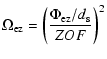
The field size being proportional to N, enough apertures are needed for fitting the observed planetary systems within the ZOF. The much wider HOF is also usable to retrieve planet images with full S/N if a multi-spectral imaging camera and software are used to remove the peak dispersion.
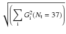
A reasonable trade-off between field size and the number of free-flyers needed involves 37 apertures. The densified pupil then resembles the aperture of a single Keck telescope, with its central obscuration removed. This optimal number N is however strongly technology-dependant. If economical ways of producing and controlling small free-flyers are developed, it may become of interest to use a larger number of smaller mirrors. With a given total collecting area, the planet/zodiacal contrast in the image does not depend on N or mirror sizes. For an exo-zodiacal cloud of size between that of the ZOF and the HOF, the planet's contrast improves with N. This follows from the expressions of signal and noise derived below. The simulations assume 37 sub-apertures, ensuring a sufficient field of view for the ZOF (
![]() with B the baseline) to image a solar system up to 25 pc in the thermal IR. A possible optical concept is described in Labeyrie (1999).
with B the baseline) to image a solar system up to 25 pc in the thermal IR. A possible optical concept is described in Labeyrie (1999).
As originally realized by Bracewell & McPhie (1978), the emission maximum of a 300 K blackbody like the Earth being close to ![]() m, this infra-red range improves the planet/star contrast. It requires a baseline of 40 to 100 m to angularly separate the planet from its star.
A coronagraphic device can be attached to the hypertelescope imager for attenuating the starlight and thus enhancing the visibility of the planet's image.
Various novel coronagraphic schemes were proposed in the past few years
for exo-planet detection (phase-mask (Roddier & Roddier 1997) or Achromatic Interfero-Coronagraph (Gay & Rabbia 1996) for instance).
In our context, we considered the Four-Quadrant Phase-Mask (FQ-PM hereafter) to be most efficient in terms of starlight rejection.
The focal plane is divided into 4 equal areas with 2 quadrants providing a
m, this infra-red range improves the planet/star contrast. It requires a baseline of 40 to 100 m to angularly separate the planet from its star.
A coronagraphic device can be attached to the hypertelescope imager for attenuating the starlight and thus enhancing the visibility of the planet's image.
Various novel coronagraphic schemes were proposed in the past few years
for exo-planet detection (phase-mask (Roddier & Roddier 1997) or Achromatic Interfero-Coronagraph (Gay & Rabbia 1996) for instance).
In our context, we considered the Four-Quadrant Phase-Mask (FQ-PM hereafter) to be most efficient in terms of starlight rejection.
The focal plane is divided into 4 equal areas with 2 quadrants providing a
![]() phase-shift (Rouan et al. 2000; Riaud et al. 2001) and as a result the bright star cancels out in the axial direction if its Airy disk is exactly centered on the mask.
A destructive interference occurs inside the geometric pupil, where an appropriate Lyot stop can block most of the diffracted starlight.
Phase-mask coronagraphy is in principle achievable with a hypertelescope
since the properties of the densified-pupil image within the ZOF are the same as for a monolithic telescope.
phase-shift (Rouan et al. 2000; Riaud et al. 2001) and as a result the bright star cancels out in the axial direction if its Airy disk is exactly centered on the mask.
A destructive interference occurs inside the geometric pupil, where an appropriate Lyot stop can block most of the diffracted starlight.
Phase-mask coronagraphy is in principle achievable with a hypertelescope
since the properties of the densified-pupil image within the ZOF are the same as for a monolithic telescope.
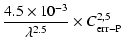
An exo-planet peak in the densified-pupil image at ![]() angular distance from the star, with
angular distance from the star, with ![]() photo-events detected per second
and per resolution element (resel) is thus contaminated by:
photo-events detected per second
and per resolution element (resel) is thus contaminated by:
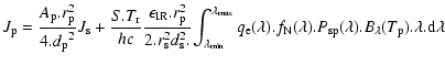
We also take into account the attenuation by the coronagraph (Fig. 1) on both the star and the planet (see Fig. 1) and also the transmission by the ZOF envelope (the diffraction lobe of a sub-pupil). Each flux is calculated in a resel ![]() .
In our calculation of the thermal and readout noise from the FPA we considered that each resel is sampled by four pixels (Shannon sampling). The global transmission includes a quantum efficiency of 45% for the detector (Rockwell Si:As detector), the filter transmission (N band
.
In our calculation of the thermal and readout noise from the FPA we considered that each resel is sampled by four pixels (Shannon sampling). The global transmission includes a quantum efficiency of 45% for the detector (Rockwell Si:As detector), the filter transmission (N band
![]() m) and an optical transmission of
m) and an optical transmission of ![]() (based on the number of mirrors reflecting 90%).
(based on the number of mirrors reflecting 90%).
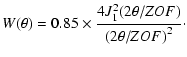
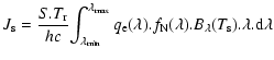
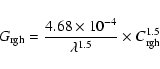
The expression of the ![]() terms are fully detailed in the Appendix. Finally, the S/N can be written as:
terms are fully detailed in the Appendix. Finally, the S/N can be written as:
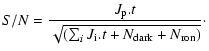 |
(2) |
Based on Eq. (2) we investigate in this section the S/N for the detection of an
Earth-like planet located in the "habitable zone", i.e. with an effective temperature
![]() K, one of the TPF ultimate goals. As a result, the distance between the star and the planet depends on the star's temperature. Since the ZOF of a hypertelescope is very small (
K, one of the TPF ultimate goals. As a result, the distance between the star and the planet depends on the star's temperature. Since the ZOF of a hypertelescope is very small (![]()
![]() in our concept), the spectral type must be considered to derive an accurate sample of target stars. For instance, an Earth-like planet orbiting around a G2V star located at 20 pc lies within the ZOF while the same planet around a F0V star will be twice farther away from the star, as will be the case also for a G2V star at 10 pc. As explained in Sect. 2.2, a planet lying outside the ZOF still provides a small spectrum in the ZOF and it is therefore important to
exploit these higher-order dispersed peaks to allow the detection of terrestrial planets for any type of stars and at any distances.
Table A.2 gives the flux then remaining in the dispersed peaks when the bandwidth is reduced to accomodate the peak dispersion (in one resel) from order 0 (inside the ZOF) to order 7.
As the planet moves away from the ZOF, the flux per resel of a higher-order peak decreases linearly owing to the spectral dispersion, while the planet's intrinsic luminosity varies as the inverse square of its distance to the observer. As a consequence, for a given spectral type, the S/N of a terrestrial planet located in the HOF is larger than in the ZOF (as seen in Fig. 2 for the F0V type).
in our concept), the spectral type must be considered to derive an accurate sample of target stars. For instance, an Earth-like planet orbiting around a G2V star located at 20 pc lies within the ZOF while the same planet around a F0V star will be twice farther away from the star, as will be the case also for a G2V star at 10 pc. As explained in Sect. 2.2, a planet lying outside the ZOF still provides a small spectrum in the ZOF and it is therefore important to
exploit these higher-order dispersed peaks to allow the detection of terrestrial planets for any type of stars and at any distances.
Table A.2 gives the flux then remaining in the dispersed peaks when the bandwidth is reduced to accomodate the peak dispersion (in one resel) from order 0 (inside the ZOF) to order 7.
As the planet moves away from the ZOF, the flux per resel of a higher-order peak decreases linearly owing to the spectral dispersion, while the planet's intrinsic luminosity varies as the inverse square of its distance to the observer. As a consequence, for a given spectral type, the S/N of a terrestrial planet located in the HOF is larger than in the ZOF (as seen in Fig. 2 for the F0V type).
![\begin{figure}
\par\includegraphics[width=7cm,clip]{MS2726f3.ps}\end{figure}](/articles/aa/full/2002/46/aa2726/img52.gif) |
Figure 3: Distribution of stars closer than 25 pc for only nine spectral types (M5V to F0V). The vertical scale at left gives the spectral type and at right the total number of stars for each spectral type. For the whole sample of 389 stars, the distances and spectral types were obtained from the Hipparcos catalogue (the Hipparcos and Tycho Catalogues 1997). |
Figure 2 shows the S/N estimated from Eq. (2) for stars belonging to 3 spectral types (F0V, G2V and M5V) located at any distance up to 25 pc. The planet peak (whatever the order of the peak) is attenuated by the windowing function towards the edge of the ZOF and by the coronagraph towards the center of the field (Fig. 1), as apparent in the S/N profiles presented in Fig. 2. Therefore, given the star's distance and spectral type the detection is optimal for a specific order. In the case of Fig. 2, Earth-like planets are detectable in order 0 for M5V stars, in order 0 and 1 for G2V stars, and from order 1 to order 5 for F0V stars.
![\begin{figure}
\par\includegraphics[width=8cm,clip]{MS2726f4.ps}\end{figure}](/articles/aa/full/2002/46/aa2726/img53.gif) |
Figure 4: Signal to noise ratio obtained for the sample of Fig. 3 with a baseline of 80 m and a zodiacal flux of 10.8 mag/''2. Earth-like planets are potentially detectable around 12% of the stars (47 stars). The exo-zodiacal flux is 10 times brighter than the zodi. |
![\begin{figure}
\par\includegraphics[width=8cm,clip]{MS2726f5.ps}\end{figure}](/articles/aa/full/2002/46/aa2726/img54.gif) |
Figure 5: Signal to noise ratio obtained for the sample of Fig. 3 with a baseline of 80 m and a zodiacal flux of 13.0 mag/''2. Earth-like planets are potentially detectable around 67% of the stars (262 stars). The exo-zodiacal flux is 10 times brighter than the zodi. |
We now consider a sample of 389 main-sequence stars (M5, M0, K5, K0, G5, G2, G0, F5 and F0) contained in the Hipparcos catalog (ESA, 1997) (see Fig. 3). The theoretical S/N obtained at
![]() m is shown in Figs. 4 and 5 with respectively a zodiacal flux of 10.8 mag/''2 (median value) and 13.0 mag/''2 (median value at the ecliptic pole). We assume a baseline of 80 m, 10 h of integration time and an exo-zodiacal cloud 10 times brighter than our zodiacal cloud. As expected, the number of potentially detectable planets is considerably affected by the intensity of the zodiacal cloud. The S/N can be larger than 10 for stars closer than 15 pc and as large as
m is shown in Figs. 4 and 5 with respectively a zodiacal flux of 10.8 mag/''2 (median value) and 13.0 mag/''2 (median value at the ecliptic pole). We assume a baseline of 80 m, 10 h of integration time and an exo-zodiacal cloud 10 times brighter than our zodiacal cloud. As expected, the number of potentially detectable planets is considerably affected by the intensity of the zodiacal cloud. The S/N can be larger than 10 for stars closer than 15 pc and as large as ![]() 300 for a nearby K0V star (
300 for a nearby K0V star (![]() Centauri). In the favorable case (Fig. 5), terrestrial planets could be detected around 67% of stars in our sample.
Centauri). In the favorable case (Fig. 5), terrestrial planets could be detected around 67% of stars in our sample.
This first sample of stars is of course biased by the selection of only 9 spectral types but was useful to investigate the optimal baseline and the effect of the zodiacal light. Then to derive realistic performance, we also carried out the same calculation for any F, G, K and M main-sequence stars (667 targets) within 25 pc with an optimal baseline of 80 m. In Table 1, we show the full sample completude in the N band (assuming each star has an Earth-like planet in orbit). Earth-like planets are potentially detectable around 73% of nearby stars in that case.
| Spectral type | F | G | K | M |
| number of stars | 62 | 217 | 193 | 195 |
| detectivity | 45% | 98% | 80% | 46% |
The interferometer baseline has also an important impact on the detectivity. Figure 6 shows the completude of the sample (fraction of detected planets) as a function of the baseline and a function of several intensities of the zodiacal cloud. As the flux of the zodiacal light decreases, the hypertelescope becomes obviously more sensitive to fainter stars, thus improving the sample completude.
The dependance with the baseline is somewhat more complex and is correlated with the zodiacal flux. The number of positive detections reaches a maximum for an optimal baseline which depends on the zodiacal flux.
For a fainter zodiacal flux (Lz=14.74 mag/2), planets are becoming detectable around fainter stars, i.e. late-type stars or distant stars. However, late-type stars are most numerous and a larger baseline (90 m) is then required to angularly separate the terrestrial planets. The maxima of the curves is then moving towards large baselines if the zodiacal flux decreases. For instance, with Lz=13 mag/''2, the maximum of detection is achieved for a baseline of ![]() 80 m and for G-type and K-type stars. With a much brighter zodi (Lz=10.8 mag/''2) the curve is almost flat because only planets around the brightest stars are detected, which means F and G stars for small baselines (
80 m and for G-type and K-type stars. With a much brighter zodi (Lz=10.8 mag/''2) the curve is almost flat because only planets around the brightest stars are detected, which means F and G stars for small baselines (![]() 40 m) and K and M nearby stars for large baselines (
40 m) and K and M nearby stars for large baselines (![]() 100 m).
100 m).
![\begin{figure}
\par\includegraphics[width=8cm,clip]{MS2726f6.ps}\end{figure}](/articles/aa/full/2002/46/aa2726/img57.gif) |
Figure 6: Percentage of detected Earth-like planets as a function of the baseline (ranging from 40 m to 100 m) and for a zodiacal flux of 10.8, 12.0, 12.7, 13.0, and 14.74 mag/''2 (Boulanger & Pérault 1988). |
Finally, we were able to estimate the most limiting source of noise in the planet's resel thanks to the calculation done in the Appendix, and we found the following noise level according to several spectral types of stars:
Some promising numerical simulations using the principle of densified-pupil imaging have been presented in Boccaletti et al. (2000). Snapshot imaging of a solar system observed from 20 pc was generated by combining the light from 36 small telescopes (
![]() cm,
cm,
![]() m) and the starlight cancellation was achieved with a phase-dot mask (Roddier & Roddier 1997).
Here we perform similar numerical simulations but using a FQ-PM to attenuate the central star. Zodiacal and exo-zodiacal backgrounds are included in the image together with co-phasing defects and mirror roughness. Figure 7 presents the result obtained with 37 telescopes, and 80 m of baseline.
The phase-mask is assumed perfectly achromatic and the interferometer has no central obscuration, which is achievable in practice by slightly off-setting the combiner optics at the focus of a large diluted mosaic mirror, whether paraboloidal or spherical.
m) and the starlight cancellation was achieved with a phase-dot mask (Roddier & Roddier 1997).
Here we perform similar numerical simulations but using a FQ-PM to attenuate the central star. Zodiacal and exo-zodiacal backgrounds are included in the image together with co-phasing defects and mirror roughness. Figure 7 presents the result obtained with 37 telescopes, and 80 m of baseline.
The phase-mask is assumed perfectly achromatic and the interferometer has no central obscuration, which is achievable in practice by slightly off-setting the combiner optics at the focus of a large diluted mosaic mirror, whether paraboloidal or spherical.
The central G2V star (mv=6.33, mN=4.70) provides a photon flux of
![]() events/s in the N filter (
events/s in the N filter (
![]() m) for a total transmission of 46%. Venus, the Earth, and Mars were added in the ZOF, Jupiter is added in the HOF. The luminosity of the zodiacal light is
m) for a total transmission of 46%. Venus, the Earth, and Mars were added in the ZOF, Jupiter is added in the HOF. The luminosity of the zodiacal light is
![]() W/(m2 sr
W/(m2 sr ![]() m) corresponding to
14.07 - 13 - 12.5 mag/''2 for respectively 8.4-10.2-12
m) corresponding to
14.07 - 13 - 12.5 mag/''2 for respectively 8.4-10.2-12 ![]() m (see Table A.4).
m (see Table A.4).
The exo-zodiacal cloud is modelled as a pair of concentric toroïdal rings with an inner diameter of
![]() AU and an outer diameter of
AU and an outer diameter of
![]() AU (see Fig. A.2) with a total intensity of 10 times the zodiacal light. The N band filter is split in three narrow-band filters (
AU (see Fig. A.2) with a total intensity of 10 times the zodiacal light. The N band filter is split in three narrow-band filters (
![]() m,
m,
![]() m and
m and
![]() m).
As seen in Fig. 7, the FQ-PM provides a sufficient rejection rate for the snapshot detection of Venus, the Earth and the dispersed peak of Jupiter with 37 sub-apertures in a total integration time of 10 hours. Mars would require a longer integration time (12 hours).
Once compared to the simulations reported in Boccaletti et al. (2000),
the FQ-PM provides a much better sensitivity than a simple phase dot for the detection of exo-planets with an hypertelescope.
Moreover, the frame subtraction of a reference star is no longer required since the diffracted light from the FQ-PM is mostly centrosymmetrical.
The opposite quadrants can be subtracted to remove a signicant part of symmetrical sources of noise (speckle pattern, or zodiacal and exo-zodiacal background).
m).
As seen in Fig. 7, the FQ-PM provides a sufficient rejection rate for the snapshot detection of Venus, the Earth and the dispersed peak of Jupiter with 37 sub-apertures in a total integration time of 10 hours. Mars would require a longer integration time (12 hours).
Once compared to the simulations reported in Boccaletti et al. (2000),
the FQ-PM provides a much better sensitivity than a simple phase dot for the detection of exo-planets with an hypertelescope.
Moreover, the frame subtraction of a reference star is no longer required since the diffracted light from the FQ-PM is mostly centrosymmetrical.
The opposite quadrants can be subtracted to remove a signicant part of symmetrical sources of noise (speckle pattern, or zodiacal and exo-zodiacal background).
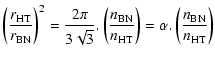
In a multi-aperture Bracewell interferometer, the beams coming out from each sub-aperture are spatially filtered and combined with beam splitters in the pupil plane. A single detector pixel receives the combined sub-aperture lobes, containing the attenuated star and the planet. The Bracewell interferometer is adjusted to provide a central dark minimum in its angular transmission map, to attenuate the star somewhat like a coronagraph does. The nulling is obtained with appropriate phase-shifts (made achromatic if possible) among the sub-apertures. A high-resolution transmission field map can then be reconstructed by rotating the interferometer around the pointing direction.
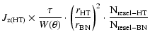
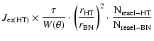
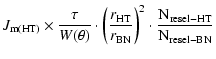
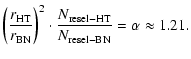
The transmission map is not uniform and we adopt an average value of
![]() (Absil 2002). This corresponds to the highest value proposed for a Bracewell nuller.
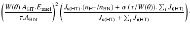
Boccaletti et al. (2000) have given analytical expressions of S/N for comparing the performance of such beam-split interferometers and hypertelescopes. We now refine the comparison by using Eq. (2).
In the following, the noise contributions in the Bracewell nuller (BN) are expressed as a function of the J terms calculated for the hypertelescope (HT). Most of the corrective factors are geometrical. The contribution of the speckle noise (
(Absil 2002). This corresponds to the highest value proposed for a Bracewell nuller.
Boccaletti et al. (2000) have given analytical expressions of S/N for comparing the performance of such beam-split interferometers and hypertelescopes. We now refine the comparison by using Eq. (2).
In the following, the noise contributions in the Bracewell nuller (BN) are expressed as a function of the J terms calculated for the hypertelescope (HT). Most of the corrective factors are geometrical. The contribution of the speckle noise (
![]() )
is not considered since it is negligible.
)
is not considered since it is negligible.
Assuming the same collecting area for both designs, the sub-aperture radii (r) are given by:
 |
(3) |
The planet flux now becomes:
 |
(4) |
The stellar level is:
 |
(5) |
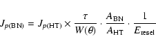
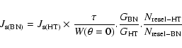
To derive the contributions of extended sources in the BN mode from the HT mode, we took into account
![]() for similar reasons as above. Also, the ratio of the sub-aperture solid angle
for similar reasons as above. Also, the ratio of the sub-aperture solid angle
![]() as well as the ratio of number of resels
as well as the ratio of number of resels
![]() .
Finally, the J terms become:
.
Finally, the J terms become:
| = |  |
(6a) | |
| = |  |
(6b) | |
| = |  |
(6c) | |
| = |  |
(6d) |
| = | (7a) | ||
| = | (7b) |
 |
(8) |
| = |  |
(9a) | |
 |
(9b) |
| Spectral type | F0V | F5V | G0V | G2V |
| maximum gain | 28 | 32 | 22 | 20 |
| Spectral type | G5V | K0V | K5V | M0V | M5V |
| maximum gain | 22 | 50 | 30 | 34 | 42 |
In this case the baseline of the hypertelescope is not optimized for all spectral types. However, as seen in Table 2, the gain in exposure time is significant with respect to the Bracewell nuller. The gain arises from
many differents points. First, the capability of the hypertelescope to spatially separate the planet peak from the background halo owing to the angular resolution, because this interferometric configuration has a wider field of view than a Bracewell nuller. The zodiacal and exo-zodiacal light is therefore much brighter than any exo-planets. To overcome this problem of FOV, the nuller has to be rotated to perform a synchronous detection assuming that the zodiacal and exo-zodiacal light is centrosymmetrical, unlike the planet peak. However, the observation of many disks does not confirm these possible centrosymmetrical exo-zodiacal clouds (see for instance the warp of ![]() Pic, Mouillet et al. 1997). With a synchronous detection, the Bracewell nuller does not always detect the planet contribution because the lower intensity of starlight residue in the transmission map must correspond to the planet peak position. The global efficiency with this type of detection is
Pic, Mouillet et al. 1997). With a synchronous detection, the Bracewell nuller does not always detect the planet contribution because the lower intensity of starlight residue in the transmission map must correspond to the planet peak position. The global efficiency with this type of detection is
![]() where
where
![]() is the number of sub-apertures of the Bracewell interferometer. The exposure time increases with the number of apertures. However, with the hypertelescope concept we have demonstrated that behaviour is exactly the opposite. Second, the attenuation factor for the planet peak
is the number of sub-apertures of the Bracewell interferometer. The exposure time increases with the number of apertures. However, with the hypertelescope concept we have demonstrated that behaviour is exactly the opposite. Second, the attenuation factor for the planet peak
![]() is always higher than
is always higher than
![]() ,
when the nulling varies as
,
when the nulling varies as ![]() ,
however with coronagraphic device the variation is in
,
however with coronagraphic device the variation is in ![]() ,
where
,
where ![]() is the angular separation of the planet compared to the parent star.
is the angular separation of the planet compared to the parent star.
As already demonstrated in Boccaletti et al. (2000) the numerical simulations presented in this article confirm that a hypertelescope with coronagraph can achieve exo-planet detection in the mid-IR, and be more sensitive than interferometers using beam-splitters in their combiner. This new series of simulations bring out some additional conclusions with respect to our previous work.
First, we show that the main drawback, the field of view limitation, can be overcome if exo-planets are detected using their secondary dispersed peaks. This makes it unnecessary to vary the array size for zooming the image, as suggested before. One can define an optimal fixed baseline according to the most frequent stellar spectral types to be observed. For instance, with a baseline of 80 m an Earth-like planet is potentially detectable around 73% of target stars in 10 hours.
Second, the comparison between the coronagraphic hypertelescope and the Bracewell nuller has been performed in more detail than in Boccaletti et al. (2000). We similarly find that the hypertelescope can be more efficient than a Bracewell nuller by at least 1 order of magnitude, in terms of the exposure time needed to detect exo-planets (see Table 2). However, it requires more sub-apertures, the size of which is smaller if equal collecting areas are considered.
Finally, the signal to noise ratio estimation presented in the Appendix is usefull to investigate the effect of each background component. We find that the dominant sources of noise when searching Earth-like planets in the mid-IR are the exo-zodiacal and zodiacal clouds. The stellar residuals, with the speckles generated by phase errors are fainter if the starlight rejection is larger than 105.
Phase-mask coronagraphy is well suited to hypertelescopes. Some ongoing experiment are addressing the technology readiness of these devices. Miniature versions of these have been tested at Observatoire de Haute-Provence, both in the laboratory and on the sky. They use diffractive Pedretti et al. (2000) or geometric-optics Gillet et al. (2002, submitted) methods of pupil densification. A four-quadrant phase mask coronagraph is also being tested. Some of us are also involved in the NGST European consortium for the study of a phase-mask coronagraph to be implemented in the imager of MIRI (mid-IR instrument) (Dubreuil et al. 2002), and obviously the issues for NGST and TPF are very similar. A first prototype was manufactured for visible wavelengths and succesfully tested on an optical bench allowing starlight rejection ![]() 45 000 in the central resel (Riaud et al. to be published) and a contrast as large as 106 at
45 000 in the central resel (Riaud et al. to be published) and a contrast as large as 106 at
![]() .
A simple phase mask, having a chromatic response, is used but achromatized versions were also recently proposed (Riaud et al. 2001 for instance) and are being studied in our group.
.
A simple phase mask, having a chromatic response, is used but achromatized versions were also recently proposed (Riaud et al. 2001 for instance) and are being studied in our group.
A subsequent step which we are preparing is the testing of a hypertelescope with a phase-mask coronagraph. Given the sensitivity gain with respect to previous forms of nulling, a hypertelescope version of the TPF should now be considered, and more detailed comparisons can be made. The direct imaging capability is also of obvious interest for a broad range of science, including the deep-field imaging of remote galaxies. Because deployable structures will be difficult to use for arrays larger than 50 or 100 m, we further explore the use of free-flyer elements driven by solar sails. Solar sails are attractive in terms of accuracy but require low masses (of less than 25 kg). The hypertelescope concept with its small mirror elements (60-70 cm) seems to be adapted to this technology. Sails also serving as multi-layer sunshields can keep the mirror elements below 40-60 K. For cost reasons, one can start with a modest hypertelescope having 7 mirror elements and then later add sub-apertures to increase the field of view and the full sample completude.
Acknowledgements
We wish to thank the DARWIN team: Alain Léger principal investigator, Alain Labèque chief enginer, Marc Ollivier and Pedrag Sékulic for helpful discussions. And also we wish to thank the referee Olivier Guyon for useful comments and corrections.
This Appendix presents additional information to derive the detailed calculation of the signal to noise ratio of an hypertelescope in the context of extra-terrestrial planets detection. In particular, we assess the terms of Eq. (2): ![]() ,
,
![]() ,
,
![]() ,
,
![]() ,
,
![]() ,
,
![]() ,
,
![]() ,
,
![]() and
and
![]() .
.
In this paper we have considered 2 possible designs using 7 and 37 sub-apertures. Several parameters of these configurations are listed in Table A.1.
| Configuration | hexagonal | |
| Number of sub-apertures | 7 | 37 |
|
Sub-aperture diameter (in m) |
1.53 | 0.66 |
| Total surface (in m2) | 10.60 | |
| Baseline (B) (in m) | 40-100 | |
|
Field of View diameter in |
|
|
|
Number of resels in the ZOF (
|
21 | 115 |
|
Energy in interference peak
|
0.65 | 0.81 |
|
Energy in
|
0.51 | 0.63 |
 |
(A.1) |
| order | 0 | 1 | 2 | 3 |
| Flux in % | 100 | 98.5 | 85.5 | 66.4 |
| Flux (spectrum) in % | 86 | 84.3 | 74 | 56.4 |
|
|
6 | 7.65 | 8.5 | 8.925 |
|
|
14 | 12.75 | 11.9 | 11.475 |
| order | 4 | 5 | 6 | 7 |
| Flux in % | 53.2 | 44.3 | 38.1 | 32.9 |
| Flux (spectrum) in % | 43.9 | 35.6 | 30.8 | 26.6 |
|
|
9.18 | 9.35 | 9.47 | 9.56 |
|
|
11.22 | 11.05 | 10.93 | 10.08 |
The star flux is obtained with the classical black-body relation (
![]() )
integrated in the N filter (
)
integrated in the N filter (
![]() m,
m,
![]() m) with a maximum transmission of 70% (
m) with a maximum transmission of 70% (
![]() ).
Assuming a Si: As Rockwell detector in the FPA with
).
Assuming a Si: As Rockwell detector in the FPA with
![]() the quantum efficiency,
the quantum efficiency, ![]() (
(
![]() )
is given by:
)
is given by:
 |
(A.2) |
Using the coronagraph, the residual starlight is:
| (A.3) |
The Earth-like spectrum results from a combination between the reflected light from the star at visible wavelength and a black-body emission in the thermal IR.
For an averaged temperature
![]() K, the distance of the planet to the star scales with the star spectral type (i.e. temperature
K, the distance of the planet to the star scales with the star spectral type (i.e. temperature ![]() and radius
and radius ![]() ):
):
 |
(A.4) |
 |
(A.5) |
Then, the flux of the planet is attenuated by the windowing function and by the coronagraph radial transmission which becomes significant for Earth-like planets around M0V since they are angularly very close:
| (A.6) |
| (A.7) |
| spectral type | F0 | F5 | G0 |
| 7240 | 6540 | 5920 | |
|
|
|
|
|
|
|
|
|
|
|
|
0.1009 | 0.1010 | 0.1011 |
|
|
18.84 | 18.32 | 17.65 |
|
|
2.792 | 1.896 | 1.207 |
| spectral type | G2 | G5 | K0 |
| 5780 | 5610 | 5240 | |
|
|
|
|
|
|
|
|
|
|
|
|
0.1011 | 0.1012 | 0.1012 |
|
|
17.31 | 17.16 | 16.66 |
|
|
1 | 0.891 | 0.642 |
| spectral type | K5 | M0 | M5 |
| 4410 | 3920 | 3120 | |
|
|
|
|
|
|
|
|
|
|
|
|
0.1013 | 0.1015 | 0.1021 |
|
|
16.25 | 15.46 | 14.76 |
|
|
0.416 | 0.245 | 0.130 |
The zodiacal light brightness observed from the Earth is given by Table 17 of
Leinert et al. (1997). Towards the ecliptic pole, the brightness is
![]() or
or
![]() mag/''2 in the N filter
and the median value is
mag/''2 in the N filter
and the median value is ![]()
![]() or
or
![]() mag/''2.
The zodiacal light is a uniform background contained within the lobe of the sub-aperture (solid angle
mag/''2.
The zodiacal light is a uniform background contained within the lobe of the sub-aperture (solid angle
![]() ), but the total energy is concentrated in
), but the total energy is concentrated in
![]() inside the ZOF owing to the densification process and is modulated by the windowing function.
The zodiacal flux in photon/s and per resel is thus given by:
inside the ZOF owing to the densification process and is modulated by the windowing function.
The zodiacal flux in photon/s and per resel is thus given by:
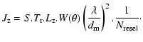 |
(A.8) |
| mag/''2 | M Jy/sr | 0 mag in Jy | |
| 8.4 | 14.07 | 18.1 | 58 |
| 10.6 | 13 | 28.8 | 36.5 |
| 12 | 12.50 | 37.0 | 28 |
| 20 | 10.33 | 102.6 | 10.4 |
| 21 | 10.11 | 113.2 | 9.4 |
![\begin{figure}
\par\includegraphics[width=8.8cm,clip]{MS2726f9.ps}\end{figure}](/articles/aa/full/2002/46/aa2726/img194.gif) |
Figure A.1:
Zodiacal background observed from the Earth (Leinert et al. 1997) in
|
The characteristics of the exo-zodiacal cloud is similar to that of the zodiacal cloud except that its extension is restricted to
![]() .
In addition, the emissivity in the thermal infra-red can be locally more important especially if the cloud is seen edge-on or contains some inhomogeneities.
The cloud is seen from the Earth with a solid angle:
.
In addition, the emissivity in the thermal infra-red can be locally more important especially if the cloud is seen edge-on or contains some inhomogeneities.
The cloud is seen from the Earth with a solid angle:
 |
(A.9) |
| (A.10) |
 |
(A.11) |
![\begin{figure}
\par\includegraphics[width=8cm,clip]{MS2726f10.ps}\hspace*{2cm}
\end{figure}](/articles/aa/full/2002/46/aa2726/img200.gif) |
Figure A.2: Exo-zodiacal intensity profile adopted in this work. The positions of Earth-like planets are shown for nine spectral type (main sequence stars). |
Cold interstellar dust (![]() K) might also be a possible source of noise. Therefore, we have verified that its effect is negligible in that context.
Its contribution in the range
K) might also be a possible source of noise. Therefore, we have verified that its effect is negligible in that context.
Its contribution in the range
![]() m is about
(0.01-1) M Jy/sr i.e. less than 3% of the zodi flux (13 mag/''2).
The interstellar dust flux (photon/s) is then:
m is about
(0.01-1) M Jy/sr i.e. less than 3% of the zodi flux (13 mag/''2).
The interstellar dust flux (photon/s) is then:
| (A.12) |
Thermal emissivity from the optical devices also contributes to the background noise. In the following, we take into account the thermal emission from the sub-apertures (
![]() ).
).
| = |  |
(A.13) | |
| = |  |
(A.14) |
| Temperature in K | 30 | 40 | 50 |
| Flux in |
|
|
|
| Temperature in K | 60 | 70 | 80 |
| Flux in |
0.16 | 3.0 | 27.5 |
The full well depth of the mid-IR camera Si:As or InSb is ![]()
![]() and is coded on 16 bits. The gain
and is coded on 16 bits. The gain ![]() is then
is then ![]()
![]() (Analog Digital Unit). Actually, at the temperature of liquid helium (4 K), the Si:As Focal Plane Array has an appreciable dark current with
(Analog Digital Unit). Actually, at the temperature of liquid helium (4 K), the Si:As Focal Plane Array has an appreciable dark current with
![]() ,
amouting to
,
amouting to
![]() or
or
![]() Zodi (
Zodi (
![]() )
for 10 hours of exposure time. Assuming a Gaussian statistic and 4 pixels per resel, we obtain:
)
for 10 hours of exposure time. Assuming a Gaussian statistic and 4 pixels per resel, we obtain:
| (A.15) |
In the thermal infra-red, existing focal plane arrays have a large readout noise (
![]() )
that can be reduce by
)
that can be reduce by ![]() if the pixel is read n times non-destructively. The readout noise can be written as
if the pixel is read n times non-destructively. The readout noise can be written as
| (A.16) |
 |
(A.17) |
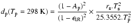
Now, it is very important to take into account the fact that with a long baseline, the star's disk is somewhat resolved even in the thermal infra-red.
For example, a F0V star at 3 pc appears with an angular
diameter of
![]() whereas a M 5 spectral type at 3 pc is only
whereas a M 5 spectral type at 3 pc is only
![]() .
The coronagraphic impact is strictly similar than for pointing errors.
The effect of pointing errors on the Four Quadrant Phase-Mask was already discussed by Rouan et al. (2000) and scales with
.
The coronagraphic impact is strictly similar than for pointing errors.
The effect of pointing errors on the Four Quadrant Phase-Mask was already discussed by Rouan et al. (2000) and scales with ![]() .
The effect of the stellar diameter is then:
.
The effect of the stellar diameter is then:
 |
(A.18) |
![]() is the function describing the stellar disc.
To simplify the calculus, we consider a star without limb darkening,
this approximation being pessimistic. The result for a G2V a star at 10 pc corresponds to a global degradation factor of
is the function describing the stellar disc.
To simplify the calculus, we consider a star without limb darkening,
this approximation being pessimistic. The result for a G2V a star at 10 pc corresponds to a global degradation factor of
![]() .
This term corresponds to the fraction of the incoming starlight
that leaks through the coronagraph.
.
This term corresponds to the fraction of the incoming starlight
that leaks through the coronagraph.
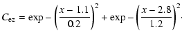
In perfect conditions, the rejection of the coronagraph can be as large as 108. This performance is degraded by the speckle noise originating from both intra-aperture phase aberrations (mirror bumpiness and tip-tilt errors) and inter-aperture piston errors. For a densified pupil, the interference peak is degraded. Its Airy rings are broken into brighter speckles and the first-order peaks at the edge of the Zero Order Field are intensified, both before and after the coronagraph.
After each cophasing adjustement, the pattern of residual speckles changes
randomly. The amplitude pattern over the pupil, including the virtual shadow pattern caused by unequal Strehl values among the sub-pupils, also creates fixed speckles in the coronagraphic image.
Numerical simulations were used to evaluate the degraded coronagraphic gain vesrus the differential piston and tip-tilt of mirror elements (
![]() and
and
![]() ), the mirror bumpiness (
), the mirror bumpiness (
![]() )
and the lack of amplitude uniformity (
)
and the lack of amplitude uniformity (
![]() ). The results are shown in Figs. A.4a, A.4b, A.3a and A.3b respectively. Power law fits are given in the following for 19 and 37 sub-apertures.
). The results are shown in Figs. A.4a, A.4b, A.3a and A.3b respectively. Power law fits are given in the following for 19 and 37 sub-apertures.
| = | (A.19a) | ||
| = |  |
(A.19b) |
| = | (A.20a) | ||
| = | (A.20b) |
 |
(A.21) |
| (A.22) | |
| (A.23) |
| = |  |
(A.24a) | |
| = | (A.24b) |
![]() has been explained above. It is the contribution of stellar diameter
and also the residual telescope jitter. We can consider in a first approximation, that the effects of
has been explained above. It is the contribution of stellar diameter
and also the residual telescope jitter. We can consider in a first approximation, that the effects of
![]() is globaly shifted by
is globaly shifted by
![]() .
The coefficient
.
The coefficient
![]() is the major contribution to the degradation factor.
is the major contribution to the degradation factor.
Finally, ![]() is the angular distance between the planet and the parent star.
is the angular distance between the planet and the parent star.
![\begin{figure}
\par\includegraphics[width=7cm,clip]{MS2726f1.ps}\end{figure}](/articles/aa/full/2002/46/aa2726/img44.gif)
![\begin{figure}
\par\includegraphics[width=7cm,clip]{MS2726f2.ps}\end{figure}](/articles/aa/full/2002/46/aa2726/img51.gif)
![\begin{figure}
\par\mbox{\includegraphics[width=5.5cm,clip]{MS2726f7.ps}\hspace{4mm}
\includegraphics[width=5.5cm,clip]{MS2726f8.ps} }\end{figure}](/articles/aa/full/2002/46/aa2726/img69.gif)
![\begin{figure}
\par\includegraphics[width=7cm,clip]{MS2726f11.ps}\hspace*{4mm}
\includegraphics[width=7cm,clip]{MS2726f12.ps}\end{figure}](/articles/aa/full/2002/46/aa2726/img221.gif)
![\begin{figure}
\par\includegraphics[width=7cm,clip]{MS2726f13.ps}\hspace*{4mm}
\includegraphics[width=7cm,clip]{MS2726f14.ps}\end{figure}](/articles/aa/full/2002/46/aa2726/img232.gif)