Osipkov (1979) and Merritt (1985) developed an inversion technique
for a special class of distribution functions that only depend on
energy and angular momentum through the combination
 |
(42) |
 |
(44) |
 |
(45) |
 |
(46) |
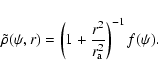
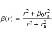
The Osipkov-Merritt models were generalized by Cuddeford (1991),
who considered models which correspond to an augmented density of
the form
 |
(47) |
 |
(48) |
| m | = |  |
(49b) |
| = |  |
(49c) |
The most interesting cases are those where ![]() is either
integer or half-integer. For integer values of
is either
integer or half-integer. For integer values of ![]() ,
the
general formula (49abc) reduces to
,
the
general formula (49abc) reduces to
For the Hernquist potential-density pair (2ab), the
augmented density corresponding to the Cuddeford formalism is
readily calculated. We obtain
First of all, it is obvious that the models with
![]() will not correspond to non-negative
distribution functions: the distribution function is already too
radial for
will not correspond to non-negative
distribution functions: the distribution function is already too
radial for ![]() (Sect. 4.2.1), and will become
even more radial for larger
(Sect. 4.2.1), and will become
even more radial for larger ![]() .
We can therefore limit the
subsequent discussion to
.
We can therefore limit the
subsequent discussion to
![]() .
Now consider
such a fixed value
.
Now consider
such a fixed value ![]() ,
and consider all Cuddeford models
corresponding to this central anisotropy. For
,
and consider all Cuddeford models
corresponding to this central anisotropy. For
![]() ,
the Cuddeford model reduces to the model
with constant anisotropy
,
the Cuddeford model reduces to the model
with constant anisotropy ![]() ,
which is physically acceptable
(Sect. 4.2.1). For
,
which is physically acceptable
(Sect. 4.2.1). For
![]() ,
the
distribution function will only consist of radial orbits, for
which the distribution function is not positive. It can therefore
be expected that, for a given value of
,
the
distribution function will only consist of radial orbits, for
which the distribution function is not positive. It can therefore
be expected that, for a given value of
![]() ,
a range of
,
a range of ![]() 's is allowed, starting from 0 up to a certain
's is allowed, starting from 0 up to a certain
![]() .
.
|
|
|
|
|
|
0.000 | |
| -1.375 | 1.764 | 0.753 |
| -1.250 | 3.598 | 0.527 |
| -1.125 | 5.550 | 0.424 |
| -1.000 | 7.582 | 0.363 |
| -0.875 | 9.680 | 0.321 |
| -0.750 | 11.83 | 0.291 |
| -0.625 | 14.02 | 0.267 |
| -0.500 | 16.23 | 0.248 |
| -0.375 | 18.51 | 0.232 |
| -0.250 | 20.57 | 0.220 |
| -0.125 | 22.61 | 0.210 |
| 0.000 | 24.42 | 0.202 |
| 0.125 | 25.87 | 0.197 |
| 0.250 | 26.70 | 0.194 |
| 0.375 | 26.42 | 0.195 |
| 0.500 | 24.00 | 0.204 |
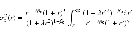
Next, we have to investigate how
![]() varies
with
varies
with ![]() ,
i.e. which anisotropy radii are allowed for a
given central anisotropy? Distribution functions with a strong
central tangential anisotropy and a small anisotropy radius are
likely to be negative. Indeed, consider the orbital structure of
such a galaxy. Because the outer regions of the galaxy
,
i.e. which anisotropy radii are allowed for a
given central anisotropy? Distribution functions with a strong
central tangential anisotropy and a small anisotropy radius are
likely to be negative. Indeed, consider the orbital structure of
such a galaxy. Because the outer regions of the galaxy
![]() are strongly radially anisotropic, the vast majority of the
stars there must be on nearly radial orbits. These stars also pass
through the central regions, where they will contribute to the
central density and radial velocity dispersion as well. The
smaller the value of
are strongly radially anisotropic, the vast majority of the
stars there must be on nearly radial orbits. These stars also pass
through the central regions, where they will contribute to the
central density and radial velocity dispersion as well. The
smaller the value of ![]() ,
i.e. the larger the value of
,
i.e. the larger the value of ![]() ,
the stronger the contribution of stars on such nearly
radial orbits. In order to create a core where the anisotropy is
tangential, a large number of stars hence have to be added which
move on tightly bound nearly circular orbits. But we are limited
from keeping on adding such stars, because we cannot exceed the
spatial density of the Hernquist profile, which has only a fairly
weak r-1 divergence. We therefore expect that no Cuddeford
models will exist beyond a certain minimal
,
the stronger the contribution of stars on such nearly
radial orbits. In order to create a core where the anisotropy is
tangential, a large number of stars hence have to be added which
move on tightly bound nearly circular orbits. But we are limited
from keeping on adding such stars, because we cannot exceed the
spatial density of the Hernquist profile, which has only a fairly
weak r-1 divergence. We therefore expect that no Cuddeford
models will exist beyond a certain minimal ![]() (except for
the degenerate case of the constant anisotropy models, which have
no radial anisotropy at large radii). Moreover, it can be expected
that for models with a tangential central anisotropy, the range of
anisotropy radii is more restricted than for models with a radial
or isotropic central anisotropy, i.e. that
(except for
the degenerate case of the constant anisotropy models, which have
no radial anisotropy at large radii). Moreover, it can be expected
that for models with a tangential central anisotropy, the range of
anisotropy radii is more restricted than for models with a radial
or isotropic central anisotropy, i.e. that
![]() is a increasing function of
is a increasing function of ![]() .
.
| |
Figure 3:
The region in
|
By numerical evaluation of the integral in Eq. (49a),
we calculated
![]() for a number of
values for
for a number of
values for ![]() (Table 1). The region in
parameter space where the Cuddeford-Hernquist models are physical
is shown in Fig. 3. Notice that all models with
(Table 1). The region in
parameter space where the Cuddeford-Hernquist models are physical
is shown in Fig. 3. Notice that all models with
![]() and
and ![]() are negative at some
point in phase space and are thus unphysical: the Hernquist
potential-density pair can support no (non-degenerate)
distribution functions of the Cuddeford type with a central
anisotropy
are negative at some
point in phase space and are thus unphysical: the Hernquist
potential-density pair can support no (non-degenerate)
distribution functions of the Cuddeford type with a central
anisotropy
![]() .
.
We are primarily interested in those models where the distribution
function can be expressed in terms of elementary functions. This
is of course possible for all half-integer values of ![]() ,
because the calculation of the distribution function involves no
integrations. Also for the integer values of
,
because the calculation of the distribution function involves no
integrations. Also for the integer values of ![]() ,
the
distribution function can be calculated analytically, through the
formula (50). Because of the limited region in
,
the
distribution function can be calculated analytically, through the
formula (50). Because of the limited region in
![]() space where Cuddeford models are non-negative,
this leaves us with four models with analytical distribution
functions, corresponding to
space where Cuddeford models are non-negative,
this leaves us with four models with analytical distribution
functions, corresponding to
![]() ,
0,
,
0,
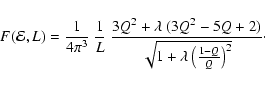
![]() and -1. The most simple of them is the case
and -1. The most simple of them is the case
![]() ,
for which we obtain
,
for which we obtain
![$\displaystyle F({\cal{E}},L)
=
\frac{1}{8\sqrt{2}\pi^3}
\left\{
\frac{3\arcsin\...
...2}}
+
\sqrt{Q}~(1-2Q)
\left[\frac{8Q^2-8Q-3}{(1-Q)^2}+8\lambda\right]
\right\},$](/articles/aa/full/2002/38/aa2799/img163.gif) |
(55) |
In Fig. 4 we show the distribution function of
the Cuddeford type for four different models. The models on the
top row have a radial central anisotropy, whereas those in the
bottom panels have a tangential anisotropy in the center. The left
and right column correspond to two different values of the
anisotropy radius. The dotted distribution functions on the
background are the distribution functions with a constant
anisotropy ![]() .
.
The character of the Cuddeford models can directly be interpreted
from these figures. Compared to the constant anisotropy models,
the Cuddeford models have a much larger fraction of stars on
radial orbits, visible for both models with radial and tangential
central anisotropy. The most conspicuous feature of each of the
Cuddeford distribution functions is that the right part of the
(r-,r+) diagram is completely empty, i.e. at large radii only
the most radial orbits are populated, which is necessary to
sustain the radial anisotropy. The boundary of the region in
turning point space beyond which no orbits are populated can be
calculated by translating the equation Q=0 in terms of the
turning points r- and r+.
 |
(56) |
| 0 | (57) | ||
| r- | 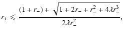 |
(58) |
 |
(59) |
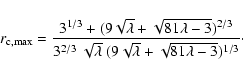
In order to calculate the radial velocity dispersion associated
with models of the Cuddeford type, we use the general formula (8a).
After some manipulation, we obtain
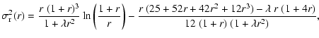 |
(61) |
In the top panels of Fig. 5 we plot the radial
velocity dispersion profiles for Hernquist-Cuddeford models, for
varying ![]() and varying
and varying ![]() (left and right panels
respectively). The behavior of
(left and right panels
respectively). The behavior of
![]() as a function of
as a function of
![]() is predictable. At small radii, the different models
have a different behavior, with the largest dispersion for the
most centrally radial models. At large radii they all have a
similar, purely radial, orbital structure, and as a consequence
their dispersion profiles all converge towards a single profile.
This limiting profile is the radial velocity dispersion profile
that corresponds to the (hypothetical) model with a completely
radial orbital structure, which we can obtain by either setting
is predictable. At small radii, the different models
have a different behavior, with the largest dispersion for the
most centrally radial models. At large radii they all have a
similar, purely radial, orbital structure, and as a consequence
their dispersion profiles all converge towards a single profile.
This limiting profile is the radial velocity dispersion profile
that corresponds to the (hypothetical) model with a completely
radial orbital structure, which we can obtain by either setting
![]() in the expression (32), or setting
in the expression (32), or setting
![]() in the expression (60),
in the expression (60),
The bottom panels of Fig. 5 show the
line-of-sight velocity dispersion of the Hernquist-Cuddeford
models. These profiles had to be calculated numerically. The
dependence of the line-of-sight dispersion upon ![]() and
and
![]() can be easily interpreted. In particular, the
line-of-sight dispersion profiles of the Cuddeford models tend
towards the line-of-sight dispersion profile of the hypothetical
purely radial Hernquist model, which reads
can be easily interpreted. In particular, the
line-of-sight dispersion profiles of the Cuddeford models tend
towards the line-of-sight dispersion profile of the hypothetical
purely radial Hernquist model, which reads
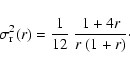
| (63) |
Copyright ESO 2002
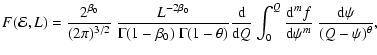
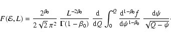
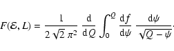
![\begin{displaymath}F({\cal{E}},L)
=
\frac{2^{\beta_0}}{(2\pi)^{3/2}}~
\frac{L...
...0}f}{{\rm d}\psi^{\frac{3}{2}-\beta_0}}
\right]_{\psi=Q}\cdot
\end{displaymath}](/articles/aa/full/2002/38/aa2799/img139.gif)
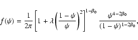
![\begin{figure}
\par\includegraphics[width=14cm,clip]{aa2799f4corr.eps}\end{figure}](/articles/aa/full/2002/38/aa2799/img157.gif)
![\begin{figure}
\par\includegraphics[width=13.4cm,clip]{MS2799f5.eps}\end{figure}](/articles/aa/full/2002/38/aa2799/img172.gif)