A&A 393, 485-497 (2002)
DOI: 10.1051/0004-6361:20021064
M. Baes![]() - H. Dejonghe
- H. Dejonghe
Sterrenkundig Observatorium, Universiteit Gent, Krijgslaan 281-S9, 9000 Gent, Belgium
Received 17 June 2002 / Accepted 12 July 2002
Abstract
Simple analytical models, such as the Hernquist model,
are very useful tools to investigate the dynamical structure of
galaxies. Unfortunately, most of the analytical distribution
functions are either isotropic or of the Osipkov-Merritt type, and
hence basically one-dimensional. We present three different
families of anisotropic distribution functions that
self-consistently generate the Hernquist potential-density pair.
These families have constant, increasing and decreasing anisotropy
profiles respectively, and can hence represent a wide variety of
orbital structures. For all of the models presented, the
distribution function and the velocity dispersions can be written
in terms of elementary functions. These models are ideal tools for
a wide range of applications, in particular to generate the
initial conditions for N-body or Monte Carlo simulations.
Key words: galaxies: kinematics and dynamics - galaxies: structure
From a stellar dynamical point of view, the most complete
description of a stellar system is the distribution function
![]() ,
which gives the probability density for the stars
in phase space. In this paper, we will concentrate on the problem
of constructing anisotropic equilibrium distribution functions
that self-consistently generate a given spherical mass density
profile
,
which gives the probability density for the stars
in phase space. In this paper, we will concentrate on the problem
of constructing anisotropic equilibrium distribution functions
that self-consistently generate a given spherical mass density
profile ![]() .
In the assumption of spherical symmetry, the
mass density of a stellar system can easily be derived from the
observed surface brightness profile, at least if we assume that
the mass-to-light ratio is constant and that dust attenuation is
negligible. And as the surface brightness of a galaxy (or bulge or
cluster) is fairly cheap and straightforward to observe, compared
to other dynamical observables which require expensive
spectroscopy, the problem we will deal with is relevant and
important.
.
In the assumption of spherical symmetry, the
mass density of a stellar system can easily be derived from the
observed surface brightness profile, at least if we assume that
the mass-to-light ratio is constant and that dust attenuation is
negligible. And as the surface brightness of a galaxy (or bulge or
cluster) is fairly cheap and straightforward to observe, compared
to other dynamical observables which require expensive
spectroscopy, the problem we will deal with is relevant and
important.
The first step in the construction of self-consistent models is
the calculation of the gravitational potential ![]() ,
which
can immediately be determined through Poisson's equation. The
second step, the actual construction of the distribution function,
is less straightforward. Basic stellar dynamics theory (see e.g. Binney & Tremaine 1987) learns that steady-state distribution
functions for spherical systems can generally be written as a
function of binding energy and angular momentum. We hence have to
determine a distribution function
,
which
can immediately be determined through Poisson's equation. The
second step, the actual construction of the distribution function,
is less straightforward. Basic stellar dynamics theory (see e.g. Binney & Tremaine 1987) learns that steady-state distribution
functions for spherical systems can generally be written as a
function of binding energy and angular momentum. We hence have to
determine a distribution function
![]() ,
such that the
zeroth order moment of this distribution function equals the
density, i.e. we have to solve the integral equation
,
such that the
zeroth order moment of this distribution function equals the
density, i.e. we have to solve the integral equation
Particularly interesting are models for which the distribution function and its moments can be computed analytically. Such models have many useful applications, which can roughly be divided into two classes. On the one hand, they can improve our general understanding of physical processes in galaxies in an elegant way. For example, they can serve as simple galaxy models, in which it is easy to generate the starting conditions for N-body or Monte Carlo simulations, or to test new data reduction or dynamical modelling techniques. A quick look at the overwhelming success of simple analytical models, such as the Plummer sphere (Plummer 1911; Dejonghe 1987), the isochrone sphere (Hénon 1959, 1960), the Jaffe model (Jaffe 1983) and the Hernquist model (Hernquist 1990), provides enough evidence. On the other hand, analytical models are also useful for the detailed dynamical modelling of galaxies. For example, in modelling techniques such as the QP technique (Dejonghe 1989), a dynamical model for an observed galaxy is built up as a linear combination of components, for each of which the distribution function and its moments are known analytically. As a result, the distribution function and the moments of the final model are also analytical, which obviously has a number of advantages.
Unfortunately, the number of dynamical models for which the distribution function is known analytically is rather modest. Moreover, most of them consist of distribution functions that are isotropic or of the Osipkov-Merritt type, and therefore basically one-dimensional. An exception is the completely analytical family of anisotropic models described by Dejonghe (1987). These models self-consistently generate the Plummer potential-density pair, a simple yet useful model for systems with a constant density core.
During the last decade, however, it has become clear that, at
small radii, elliptical galaxies usually have central density
profiles that behave as
![]() with
with
![]() (Lauer et al. 1995; Gebhardt et al. 1996). Such galaxies can
obviously not be adequately modelled with a constant density core.
This has stimulated the quest for simple potential-density pairs,
and corresponding distribution functions, with a central density
cusp. The first effort to construct such models was undertaken by
Ciotti (1991) and Ciotti & Lanzoni (1997), who discussed the the
dynamical structure of stellar systems following the R1/m law
(Sérsic 1968), a natural generalization of the empirical
R1/4 law of de Vaucouleurs (1948). A major drawback of this
family, however, is that the spatial density and the distribution
function can not be written in terms of elementary functions (see
Mazure & Capelato 2002). A more useful family is formed by the
so-called
(Lauer et al. 1995; Gebhardt et al. 1996). Such galaxies can
obviously not be adequately modelled with a constant density core.
This has stimulated the quest for simple potential-density pairs,
and corresponding distribution functions, with a central density
cusp. The first effort to construct such models was undertaken by
Ciotti (1991) and Ciotti & Lanzoni (1997), who discussed the the
dynamical structure of stellar systems following the R1/m law
(Sérsic 1968), a natural generalization of the empirical
R1/4 law of de Vaucouleurs (1948). A major drawback of this
family, however, is that the spatial density and the distribution
function can not be written in terms of elementary functions (see
Mazure & Capelato 2002). A more useful family is formed by the
so-called ![]() -models (Dehnen 1993; Tremaine et al. 1994),
characterized by a density proportional to r-4 at large radii
and a divergence in the center as
-models (Dehnen 1993; Tremaine et al. 1994),
characterized by a density proportional to r-4 at large radii
and a divergence in the center as
![]() with
with
![]() .
The dynamical structure of models with this
potential-density pair has been extensively investigated (e.g. Carollo et al. 1995; Ciotti 1996; Meza &
Zamorano 1997), but only for isotropic or Osipkov-Merritt type
distribution functions. Simple analytical models with a more
general anisotropy structure are still lacking.
.
The dynamical structure of models with this
potential-density pair has been extensively investigated (e.g. Carollo et al. 1995; Ciotti 1996; Meza &
Zamorano 1997), but only for isotropic or Osipkov-Merritt type
distribution functions. Simple analytical models with a more
general anisotropy structure are still lacking.
In this paper we construct a number of families of completely
analytical anisotropic dynamical models that self-consistently
generate the Hernquist (1990) potential-density pair. It is a
special case of the family of ![]() -models, corresponding to
-models, corresponding to
![]() .
In dimensionless units, the Hernquist
potential-density pair is given by 010
.
In dimensionless units, the Hernquist
potential-density pair is given by 010
As the density diverges as 1/r for
![]() ,
the surface
brightness I(R) will diverge logarithmically for
,
the surface
brightness I(R) will diverge logarithmically for
![]() .
More precisely, the surface brightness profile
has the form
.
More precisely, the surface brightness profile
has the form
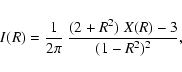 |
(3) |
A general discussion on the inversion of the fundamental Eq. (1),
and hence on the construction anisotropic
distribution functions for a given spherical potential-density
pair, is presented by Dejonghe (1986). The key ingredient of the
inversion procedure is the concept of the augmented mass density
![]() ,
which is a function of potential and
radius, such that the condition
,
which is a function of potential and
radius, such that the condition
Besides providing a nice way to generate a distribution function
for a given potential-density pair, the augmented density is also
very useful to calculate the moments of the distribution function.
The anisotropic moments are defined as
By means of these functions, we can define the anisotropy
![]() as
as
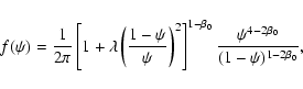
The simplest dynamical models are those where the augmented
density is a function of the potential only,
![]() .
For such models, the
distribution function is only a function of the binding energy,
i.e. the distribution function is isotropic. In this case, the
integral Eq. (1) can be inverted to find the
well-known Eddington relation
.
For such models, the
distribution function is only a function of the binding energy,
i.e. the distribution function is isotropic. In this case, the
integral Eq. (1) can be inverted to find the
well-known Eddington relation
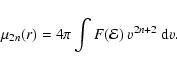 |
(13) |
The isotropic model that corresponds to the potential-density pair (2ab)
is described in full detail by Hernquist (1990).
We restrict ourselves by resuming the most important results, for
a comparison with the anisotropic models discussed later in this
paper. The augmented density reads
 |
(18) |
| |
= | ||
| (21) |
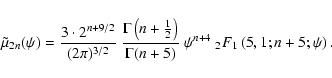
A special family of distribution functions that can easily be
generated using the technique outlined in Sect. 2 corresponds to
models with a density that depends on r only through a factor
![]() ,
i.e.
,
i.e.
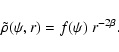 |
(22) |
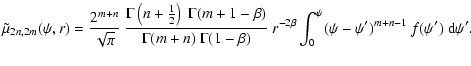 |
(25) |
![\begin{figure}
\par\includegraphics[width=13.4cm,clip]{MS2799f1.eps}\end{figure}](/articles/aa/full/2002/38/aa2799/img81.gif) |
Figure 1:
The distribution function of the Hernquist models with a
constant anisotropy, represented as isoprobability contours in
turning point space. The distribution functions in solid lines
represent a radial model with
|
| Open with DEXTER | |
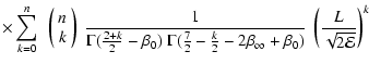
Applying the formula (23) to the Hernquist
potential-density pair (2ab) yields
It is no surprise that the distribution function is not positive
for the largest possible values of ![]() ,
because models where
only the radial orbits are populated can only be supported by a
density profile that diverges as r-2 or steeper in the center
(Richstone & Tremaine 1984). It turns out that the distribution
function (28) is everywhere non-negative for
,
because models where
only the radial orbits are populated can only be supported by a
density profile that diverges as r-2 or steeper in the center
(Richstone & Tremaine 1984). It turns out that the distribution
function (28) is everywhere non-negative for
![]() .
.
For all integer and half-integer values of ![]() ,
the
hypergeometric series in (28) can be expressed in terms
of elementary functions. Very useful are half-integer values of
,
the
hypergeometric series in (28) can be expressed in terms
of elementary functions. Very useful are half-integer values of
![]() ,
because the energy-dependent part of the distribution
function can then be written as a rational function of
,
because the energy-dependent part of the distribution
function can then be written as a rational function of
![]() .
For integer values of
.
For integer values of ![]() ,
the hypergeometric
series can be written as a function containing integer and
half-integer powers of
,
the hypergeometric
series can be written as a function containing integer and
half-integer powers of ![]() and
and
![]() and a factor
and a factor
![]() ,
similar to the isotropic distribution
function (17).
,
similar to the isotropic distribution
function (17).
The limiting model
![]() is particularly simple. It
has an augmented density that is a power law of potential and
radius,
is particularly simple. It
has an augmented density that is a power law of potential and
radius,
 |
(29) |
In Fig. 1 we compare the distribution functions
of the radial model with
![]() and the tangential
model with
and the tangential
model with ![]() with the distribution function of the
isotropic Hernquist model. The distribution functions are shown by
means of their isoprobability contours in turning point space,
which can easily be interpreted in terms of orbits. Compared to
the isotropic model, the radial model prefers orbits on the upper
left side of the diagram, with an apocenter much larger than the
pericenter, i.e. elongated orbits. The isoprobability contours of
tangential models on the other hand lean towards the diagonal axes
where pericenter and apocenter are equal, i.e. nearly-circular
orbits are preferred.
with the distribution function of the
isotropic Hernquist model. The distribution functions are shown by
means of their isoprobability contours in turning point space,
which can easily be interpreted in terms of orbits. Compared to
the isotropic model, the radial model prefers orbits on the upper
left side of the diagram, with an apocenter much larger than the
pericenter, i.e. elongated orbits. The isoprobability contours of
tangential models on the other hand lean towards the diagonal axes
where pericenter and apocenter are equal, i.e. nearly-circular
orbits are preferred.
By means of substituting the expression (27) into the
general formula (7), we can derive an analytical
expression for all moments of the distribution function,
| |
= |  |
|
| (31) |
![\begin{figure}
\par\includegraphics[width=6.3cm,clip]{MS2799f2.eps}\end{figure}](/articles/aa/full/2002/38/aa2799/img105.gif) |
Figure 2:
The velocity dispersion of the Hernquist models with a
constant anisotropy. The upper and lower panels show the radial
velocity dispersions
|
| Open with DEXTER | |
Particular cases are the models that correspond to the most radial
and tangential distribution functions. On the one hand, the limit
case
![]() has the simple velocity dispersion
profiles
has the simple velocity dispersion
profiles
 |
(35) |
The line-of-sight velocity dispersion for anisotropic models is
found through the formula
 |
(36) |
| |
= | ||
| (39) |
| |
= |  |
|
| (40) |
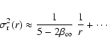
In the bottom panel of Fig. 2 we plot the
line-of-sight dispersion profiles for a number of different values
of ![]() .
The behavior of the individual profiles is analogous
to the spatial dispersion profiles: except for the
.
The behavior of the individual profiles is analogous
to the spatial dispersion profiles: except for the
![]() model, which has a finite central dispersion,
the
model, which has a finite central dispersion,
the
![]() profiles start at zero in the center, rise strongly
until a certain maximum and then decrease smoothly towards zero at
large projected radii. The behavior for
profiles start at zero in the center, rise strongly
until a certain maximum and then decrease smoothly towards zero at
large projected radii. The behavior for ![]() can be quantified
if we introduce the asymptotic expansion (33) into the
formula (38),
can be quantified
if we introduce the asymptotic expansion (33) into the
formula (38),
Osipkov (1979) and Merritt (1985) developed an inversion technique
for a special class of distribution functions that only depend on
energy and angular momentum through the combination
 |
(42) |
 |
(44) |
 |
(45) |
 |
(46) |
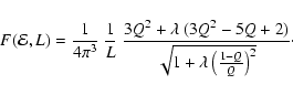
The Osipkov-Merritt models were generalized by Cuddeford (1991),
who considered models which correspond to an augmented density of
the form
 |
(47) |
 |
(48) |
| m | = |  |
(49b) |
| = |  |
(49c) |
The most interesting cases are those where ![]() is either
integer or half-integer. For integer values of
is either
integer or half-integer. For integer values of ![]() ,
the
general formula (49abc) reduces to
,
the
general formula (49abc) reduces to
For the Hernquist potential-density pair (2ab), the
augmented density corresponding to the Cuddeford formalism is
readily calculated. We obtain
First of all, it is obvious that the models with
![]() will not correspond to non-negative
distribution functions: the distribution function is already too
radial for
will not correspond to non-negative
distribution functions: the distribution function is already too
radial for ![]() (Sect. 4.2.1), and will become
even more radial for larger
(Sect. 4.2.1), and will become
even more radial for larger ![]() .
We can therefore limit the
subsequent discussion to
.
We can therefore limit the
subsequent discussion to
![]() .
Now consider
such a fixed value
.
Now consider
such a fixed value ![]() ,
and consider all Cuddeford models
corresponding to this central anisotropy. For
,
and consider all Cuddeford models
corresponding to this central anisotropy. For
![]() ,
the Cuddeford model reduces to the model
with constant anisotropy
,
the Cuddeford model reduces to the model
with constant anisotropy ![]() ,
which is physically acceptable
(Sect. 4.2.1). For
,
which is physically acceptable
(Sect. 4.2.1). For
![]() ,
the
distribution function will only consist of radial orbits, for
which the distribution function is not positive. It can therefore
be expected that, for a given value of
,
the
distribution function will only consist of radial orbits, for
which the distribution function is not positive. It can therefore
be expected that, for a given value of
![]() ,
a range of
,
a range of ![]() 's is allowed, starting from 0 up to a certain
's is allowed, starting from 0 up to a certain
![]() .
.
|
|
|
|
|
|
0.000 | |
| -1.375 | 1.764 | 0.753 |
| -1.250 | 3.598 | 0.527 |
| -1.125 | 5.550 | 0.424 |
| -1.000 | 7.582 | 0.363 |
| -0.875 | 9.680 | 0.321 |
| -0.750 | 11.83 | 0.291 |
| -0.625 | 14.02 | 0.267 |
| -0.500 | 16.23 | 0.248 |
| -0.375 | 18.51 | 0.232 |
| -0.250 | 20.57 | 0.220 |
| -0.125 | 22.61 | 0.210 |
| 0.000 | 24.42 | 0.202 |
| 0.125 | 25.87 | 0.197 |
| 0.250 | 26.70 | 0.194 |
| 0.375 | 26.42 | 0.195 |
| 0.500 | 24.00 | 0.204 |
Next, we have to investigate how
![]() varies
with
varies
with ![]() ,
i.e. which anisotropy radii are allowed for a
given central anisotropy? Distribution functions with a strong
central tangential anisotropy and a small anisotropy radius are
likely to be negative. Indeed, consider the orbital structure of
such a galaxy. Because the outer regions of the galaxy
,
i.e. which anisotropy radii are allowed for a
given central anisotropy? Distribution functions with a strong
central tangential anisotropy and a small anisotropy radius are
likely to be negative. Indeed, consider the orbital structure of
such a galaxy. Because the outer regions of the galaxy
![]() are strongly radially anisotropic, the vast majority of the
stars there must be on nearly radial orbits. These stars also pass
through the central regions, where they will contribute to the
central density and radial velocity dispersion as well. The
smaller the value of
are strongly radially anisotropic, the vast majority of the
stars there must be on nearly radial orbits. These stars also pass
through the central regions, where they will contribute to the
central density and radial velocity dispersion as well. The
smaller the value of ![]() ,
i.e. the larger the value of
,
i.e. the larger the value of ![]() ,
the stronger the contribution of stars on such nearly
radial orbits. In order to create a core where the anisotropy is
tangential, a large number of stars hence have to be added which
move on tightly bound nearly circular orbits. But we are limited
from keeping on adding such stars, because we cannot exceed the
spatial density of the Hernquist profile, which has only a fairly
weak r-1 divergence. We therefore expect that no Cuddeford
models will exist beyond a certain minimal
,
the stronger the contribution of stars on such nearly
radial orbits. In order to create a core where the anisotropy is
tangential, a large number of stars hence have to be added which
move on tightly bound nearly circular orbits. But we are limited
from keeping on adding such stars, because we cannot exceed the
spatial density of the Hernquist profile, which has only a fairly
weak r-1 divergence. We therefore expect that no Cuddeford
models will exist beyond a certain minimal ![]() (except for
the degenerate case of the constant anisotropy models, which have
no radial anisotropy at large radii). Moreover, it can be expected
that for models with a tangential central anisotropy, the range of
anisotropy radii is more restricted than for models with a radial
or isotropic central anisotropy, i.e. that
(except for
the degenerate case of the constant anisotropy models, which have
no radial anisotropy at large radii). Moreover, it can be expected
that for models with a tangential central anisotropy, the range of
anisotropy radii is more restricted than for models with a radial
or isotropic central anisotropy, i.e. that
![]() is a increasing function of
is a increasing function of ![]() .
.
| |
Figure 3:
The region in
|
| Open with DEXTER | |
![\begin{figure}
\par\includegraphics[width=14cm,clip]{aa2799f4corr.eps}\end{figure}](/articles/aa/full/2002/38/aa2799/img157.gif) |
Figure 4:
Comparison of the distribution function corresponding to
Hernquist models of the Cuddeford type and Hernquist models with a
constant anisotropy. The distribution functions are represented as
isoprobability contours in turning point space. The solid lines
correspond to the Cuddeford distribution functions, with the
parameters |
| Open with DEXTER | |
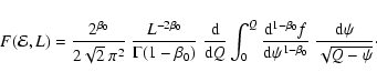
By numerical evaluation of the integral in Eq. (49a),
we calculated
![]() for a number of
values for
for a number of
values for ![]() (Table 1). The region in
parameter space where the Cuddeford-Hernquist models are physical
is shown in Fig. 3. Notice that all models with
(Table 1). The region in
parameter space where the Cuddeford-Hernquist models are physical
is shown in Fig. 3. Notice that all models with
![]() and
and ![]() are negative at some
point in phase space and are thus unphysical: the Hernquist
potential-density pair can support no (non-degenerate)
distribution functions of the Cuddeford type with a central
anisotropy
are negative at some
point in phase space and are thus unphysical: the Hernquist
potential-density pair can support no (non-degenerate)
distribution functions of the Cuddeford type with a central
anisotropy
![]() .
.
We are primarily interested in those models where the distribution
function can be expressed in terms of elementary functions. This
is of course possible for all half-integer values of ![]() ,
because the calculation of the distribution function involves no
integrations. Also for the integer values of
,
because the calculation of the distribution function involves no
integrations. Also for the integer values of ![]() ,
the
distribution function can be calculated analytically, through the
formula (50). Because of the limited region in
,
the
distribution function can be calculated analytically, through the
formula (50). Because of the limited region in
![]() space where Cuddeford models are non-negative,
this leaves us with four models with analytical distribution
functions, corresponding to
space where Cuddeford models are non-negative,
this leaves us with four models with analytical distribution
functions, corresponding to
![]() ,
0,
,
0,
![]() and -1. The most simple of them is the case
and -1. The most simple of them is the case
![]() ,
for which we obtain
,
for which we obtain
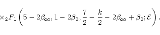
![$\displaystyle F({\cal{E}},L)
=
\frac{1}{8\sqrt{2}\pi^3}
\left\{
\frac{3\arcsin\...
...2}}
+
\sqrt{Q}~(1-2Q)
\left[\frac{8Q^2-8Q-3}{(1-Q)^2}+8\lambda\right]
\right\},$](/articles/aa/full/2002/38/aa2799/img163.gif) |
(55) |
In Fig. 4 we show the distribution function of
the Cuddeford type for four different models. The models on the
top row have a radial central anisotropy, whereas those in the
bottom panels have a tangential anisotropy in the center. The left
and right column correspond to two different values of the
anisotropy radius. The dotted distribution functions on the
background are the distribution functions with a constant
anisotropy ![]() .
.
The character of the Cuddeford models can directly be interpreted
from these figures. Compared to the constant anisotropy models,
the Cuddeford models have a much larger fraction of stars on
radial orbits, visible for both models with radial and tangential
central anisotropy. The most conspicuous feature of each of the
Cuddeford distribution functions is that the right part of the
(r-,r+) diagram is completely empty, i.e. at large radii only
the most radial orbits are populated, which is necessary to
sustain the radial anisotropy. The boundary of the region in
turning point space beyond which no orbits are populated can be
calculated by translating the equation Q=0 in terms of the
turning points r- and r+.
 |
(56) |
| 0 | (57) | ||
| r- |  |
(58) |
 |
(59) |
![\begin{figure}
\par\includegraphics[width=13.4cm,clip]{MS2799f5.eps}\end{figure}](/articles/aa/full/2002/38/aa2799/img172.gif) |
Figure 5:
The radial (upper panels) and line-of-sight (lower
panels) velocity dispersion profiles of the Hernquist-Cuddeford
models. The different curves in the two left panels correspond to
models with the same anisotropy radius |
| Open with DEXTER | |
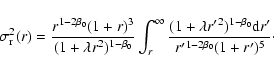
In order to calculate the radial velocity dispersion associated
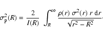
with models of the Cuddeford type, we use the general formula (8a).
After some manipulation, we obtain
 |
(61) |
In the top panels of Fig. 5 we plot the radial
velocity dispersion profiles for Hernquist-Cuddeford models, for
varying ![]() and varying
and varying ![]() (left and right panels
respectively). The behavior of
(left and right panels
respectively). The behavior of
![]() as a function of
as a function of
![]() is predictable. At small radii, the different models
have a different behavior, with the largest dispersion for the
most centrally radial models. At large radii they all have a
similar, purely radial, orbital structure, and as a consequence
their dispersion profiles all converge towards a single profile.
This limiting profile is the radial velocity dispersion profile
that corresponds to the (hypothetical) model with a completely
radial orbital structure, which we can obtain by either setting
is predictable. At small radii, the different models
have a different behavior, with the largest dispersion for the
most centrally radial models. At large radii they all have a
similar, purely radial, orbital structure, and as a consequence
their dispersion profiles all converge towards a single profile.
This limiting profile is the radial velocity dispersion profile
that corresponds to the (hypothetical) model with a completely
radial orbital structure, which we can obtain by either setting
![]() in the expression (32), or setting
in the expression (32), or setting
![]() in the expression (60),
in the expression (60),
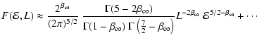
The bottom panels of Fig. 5 show the
line-of-sight velocity dispersion of the Hernquist-Cuddeford
models. These profiles had to be calculated numerically. The
dependence of the line-of-sight dispersion upon ![]() and
and
![]() can be easily interpreted. In particular, the
line-of-sight dispersion profiles of the Cuddeford models tend
towards the line-of-sight dispersion profile of the hypothetical
purely radial Hernquist model, which reads
can be easily interpreted. In particular, the
line-of-sight dispersion profiles of the Cuddeford models tend
towards the line-of-sight dispersion profile of the hypothetical
purely radial Hernquist model, which reads
| (63) |
In order to construct dynamical models with a decreasing
anisotropy, i.e. with a tangentially anisotropic halo, no special
inversion techniques exist, such that we have to rely on the
general formulae of Dejonghe (1986) to invert the fundamental
integral Eq. (1). A disadvantage is that these
formulae are numerically unstable. Their usefulness is therefore
actually restricted to analytical models. But this is not
straightforward: a direct application of the inversion formulae to
an arbitrary analytical augmented density
![]() ,
even if its looks rather simple, can result in a cumbersome
mathematical exercise, because the inversion formulae are quite
elaborate.
,
even if its looks rather simple, can result in a cumbersome
mathematical exercise, because the inversion formulae are quite
elaborate.
A useful strategy to construct models with a tangential halo
without the need to cope with the complicated general formulae, is
to profit from the linearity of the integral
Eq. (1). In particular, it is very interesting to generate
augmented densities
![]() ,
which can be expanded
in a series of functions
,
which can be expanded
in a series of functions
![]() ,
which depend on
r only through a power law,
,
which depend on
r only through a power law,
Equivalently, the moments of the distribution function can be derived from the series expansion.
For every potential ![]() ,
we can create an infinite number of
functions
,
we can create an infinite number of
functions ![]() which satisfy the identity
which satisfy the identity
![]() .
For the Hernquist potential, we can easily
create such a one-parameter family of functions
.
For the Hernquist potential, we can easily
create such a one-parameter family of functions
![]() ,
,
![\begin{displaymath}Z_n(\psi,r)
=
\left[\psi~(1+r)\right]^n
\equiv
1,
\end{displaymath}](/articles/aa/full/2002/38/aa2799/img188.gif) |
(66) |
with
![]() .
The reason why we chose
.
The reason why we chose ![]() and
and
![]() as parameters becomes clear when we look at the
expression for the anisotropy corresponding to this family of
density functions - for the moment being without bothering
whether the density corresponds to a physically acceptable
distribution function. By means of the formula (11),
we obtain
as parameters becomes clear when we look at the
expression for the anisotropy corresponding to this family of
density functions - for the moment being without bothering
whether the density corresponds to a physically acceptable
distribution function. By means of the formula (11),
we obtain
 |
(70) |
![\begin{figure}
\par\includegraphics[width=6.5cm,clip]{MS2799f6.eps}\end{figure}](/articles/aa/full/2002/38/aa2799/img200.gif) |
Figure 6:
Comparison of the distribution function corresponding to
Hernquist model with increasing anisotropy with
|
| Open with DEXTER | |
We can calculate the distribution function of these models by
applying the recipe (65b) to each of the components (69ab).
We obtain after some algebra
An interesting characteristic of these models is revealed when we
look at the asymptotic behavior of the distribution function at
large radii, i.e. for
![]() .
The term
corresponding to k=n will contribute the dominant term in the
sum (71), such that we obtain
.
The term
corresponding to k=n will contribute the dominant term in the
sum (71), such that we obtain
Finally, notice that there is no analogue for this behavior at
small radii: not all models with a fixed ![]() will have a
similar behavior for
will have a
similar behavior for
![]() ,
i.e. at small
radii.
,
i.e. at small
radii.
![\begin{figure}
\par\includegraphics[width=6.3cm,clip]{MS2799f7.eps}\end{figure}](/articles/aa/full/2002/38/aa2799/img210.gif) |
Figure 7:
The radial (upper panel) and line-of-sight (lower panel)
velocity dispersion profiles of Hernquist models with a decreasing
anisotropy. All models have the same tangential outer anisotropy
|
| Open with DEXTER | |
In order to calculate the velocity dispersion profiles of the
models of this type, we have various possibilities. We can either
calculate the dispersion for each of the n terms (69a)
through formula (26) and sum the
results, or directly apply the general recipe (8ab)
on the expression (68). In either case, we obtain an
expression very akin to the expression (32) of the
models with constant anisotropy,
 |
(73) |
Not as a surprise, the asymptotic expressions for
![]() for
for ![]() read
read
 |
(74) |
The calculation of the line-of-sight velocity dispersion is also
similar to the case of constant anisotropy. It is found that
![]() can be written in terms of elementary functions for
all integer and half-integer values of
can be written in terms of elementary functions for
all integer and half-integer values of ![]() ,
and that the
asymptotic behavior for
,
and that the
asymptotic behavior for ![]() reads
reads
 |
(75) |
Three new families of anisotropic dynamical models have been presented that self-consistently generate the Hernquist potential-density pair. For all models, in particular for the Cuddeford models of Sect. 5, we checked the conditions on the adopted parameters such that the distribution is positive, and hence physically acceptable, in phase space.
They host a wide variety of orbital structures: in general, the models presented can have an arbitrary central anisotropy, and a outer halo with the same anisotropy, a purely radial orbital structure, or an arbitrary, but more tangential, anisotropy. In order to produce models that have an arbitrary anisotropy in the central regions, and a more radial, but not purely radial, anisotropy at large radii, the most cost-effective way seems to construct a linear combination of a number of `component' dynamical models, such as the ones presented here. This technique has been adopted for several years in the QP formalism (Dejonghe 1989, for an overview see Dejonghe et al. 2001), where most of the components in the program libraries have an intrinsically tangential orbital structure.
For all of the presented models, we have analytical expressions for the distribution function and the velocity dispersions in terms of elementary functions. They are hence ideal tools for a wide range of applications, for example to generate the initial conditions for N-body or Monte Carlo simulations. At this point, a number of remarks are appropriate.
First, very few elliptical galaxies are perfectly spherical; actually, various observational and theoretical evidence suggests that many elliptical galaxies are at least moderately triaxial (Dubinski & Carlberg 1991; Hernquist 1993; Tremblay & Merritt 1995; Bak & Statler 2000). Unfortunately, an extension of the presented techniques to construct analytical axisymmetric or triaxial systems is not obvious, because the internal dynamics of such stellar systems is much more complicated than in the spherical case. Nevertheless, our models can be used as an onset to construct numerical axisymmetric of triaxial distribution functions with different internal dynamical structures, for example by the adiabatic squeezing technique presented by Holley-Bockelmann et al. (2001).
Second, the models presented here are self-consistent models,
whereas it is nowadays believed that most elliptical galaxies
contain dark matter, either in the form of a central black hole
(Merritt & Ferrarese 2001 and references therein) and/or a dark
halo (Kronawitter et al. 2000; Magorrian & Ballantyne 2001).
When constructing dynamical models with dark matter, an extra
component must be added to the gravitational potential. For
example, Ciotti (1996) constructed analytical two-component models
in which both the stellar and dark matter components have a
Hernquist density profile and an Osipkov-Merritt type distribution
function. The models presented in this paper can also be extended
to contain a dark halo or a central black hole. Indeed, the
adopted inversion techniques are perfectly suitable for this,
because the augmented density functions
![]() do
not necessarily need to satisfy the self-consistency condition (5).
Adding an extra term to the potential does not
conceptually change the character of the inversion, but it might
complicate the mathematical exercise.
do
not necessarily need to satisfy the self-consistency condition (5).
Adding an extra term to the potential does not
conceptually change the character of the inversion, but it might
complicate the mathematical exercise.
Third, we have not discussed stability issues for the presented
models. The study of the stability of anisotropic stellar systems
is difficult, and a satisfactory criterion can not easily be
given. For stability against radial perturbations, we can apply
the sufficient criterions of Antonov (1962) or Dorémus & Feix
(1973), but numerical simulations have shown that these criteria
are rather crude (Dejonghe & Merritt 1988; Meza & Zamorano
1997). Moreover, the only instability that is thought to be
effective in realistic galaxies is the so-called radial orbit
instability, an instability that drives galaxies with a large
number of radial orbits to forming a bar (Hénon 1973; Palmer &
Papaloizou 1987; Cincotta et al. 1996). The behavior of
galaxy models against perturbations of this kind can only be
tested with detailed N-body simulations or numerical linear
stability analysis. Meza & Zamorano (1997) used N-body
simulations to investigate the radial orbit instability for a
number of spherical models of the Osipkov-Merritt type, including
the Hernquist model. They found that the models are unstable for
![]() ,
which significantly restricts the set of models
that correspond to positive distribution functions (see Table 1).
It would be interesting to extend this
investigation to the three families of Hernquist models presented
in this paper, but this falls beyond the scope of this paper.
,
which significantly restricts the set of models
that correspond to positive distribution functions (see Table 1).
It would be interesting to extend this
investigation to the three families of Hernquist models presented
in this paper, but this falls beyond the scope of this paper.
Acknowledgements
The authors are grateful to Andrés Meza for a careful check on the formulae derived in this paper. Fortran codes to evaluate the internal and projected dynamics of the presented models are available from the authors.
![$\displaystyle \tilde{\mu}_{2n,2m}(\psi,r)
=
\frac{2^{m+n}}{\sqrt{\pi}}~
\frac{\...
...m}}{({\rm d}r^2)^{m}}
\left[
r^{2m}~\tilde{\rho}(\psi',r)
\right]
{\rm d}\psi'.$](/articles/aa/full/2002/38/aa2799/img47.gif)
![$\displaystyle \frac{2}{\rho(r)}
\int_0^{\psi(r)}
\frac{{\rm d}}{{\rm d}r^2}
\left[r^2~\tilde{\rho}(\psi',r)\right]
{\rm d}\psi'.$](/articles/aa/full/2002/38/aa2799/img51.gif)
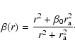
![\begin{displaymath}\beta(r)
=
1-\frac{1}{g(r)}~\frac{{\rm d}}{{\rm d}r^2}
\left[r^2~g(r)\right],
\end{displaymath}](/articles/aa/full/2002/38/aa2799/img55.gif)
![$\displaystyle F({\cal{E}})
=
\frac{1}{8\sqrt{2}\pi^3}
\left[
\frac{\sqrt{{\cal{...
...cal{E}})^2}
+
\frac{3\arcsin\sqrt{{\cal{E}}}}{(1-{\cal{E}})^{5/2}}
\right]\cdot$](/articles/aa/full/2002/38/aa2799/img63.gif)
![\begin{displaymath}F({\cal{E}},L)
=
\frac{2^{\beta_0}}{(2\pi)^{3/2}}~
\frac{L...
...0}f}{{\rm d}\psi^{\frac{3}{2}-\beta_0}}
\right]_{\psi=Q}\cdot
\end{displaymath}](/articles/aa/full/2002/38/aa2799/img139.gif)