Appendix C: 2D log-normal cascade

For any function , f can be written under the form

$$f(x,y)=\sum ^{N}_{j=0}~ \sum ^{2^{N-j}-1}_{m,n=0}~ \sum ^{3}_{k=0}c_{j,m,n}^{k}\psi _{j,m,n}^{k}(x,y).$$

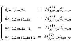
The construction rule is the following: one generates the modulus of the wavelet coefficients in a recursive way by:

$$\left\{ \begin{array}{lcr} d_{j-1,2m,2n} & = & M^{(1)}_{j,m,n... ...,2m+1,2n+1} & = & M^{(4)}_{j,m,n}d_{j,m,n}. \end{array}\right.$$

M_j,m,n follows the prescribed log-normal law .

The wavelet coefficients themselves are computed via two angles :

$$\left\{ \begin{array}{lcl} c^{1}_{j,m,n} & = & \cos(\phi )\co... ...m] c^{3}_{j,m,n} & = & \sin(\phi )d_{j,m,n} \end{array}\right.$$

where is randomly chosen between and is randomly chosen between where satisfies

$$\frac{\sin \left( 2\phi ^{*}\right) }{4\phi ^{*}}=\frac{2^{\tau (2)/2+3}}{1+2^{\tau (2)/2+3}}-\frac{1}{2}$$

with

$$\tau (q)=-\frac{\sigma ^{2}}{2}q^{2}-mq-2.$$

Finally, isotropy follows from adjusting the weights at the largest scale:

c¹_0,0,0 = d_0,0,0, c²_0,0,0 = d_0,0,0, and $c^{3}_{0,0,0} = 2^{-(\tau (2)/4+1)}d_{0,0,0}$ (see Decoster et al. 2000 for all details).