

Up: HD 152248: Evidence for interaction
Subsections
The inspection of our data reveals that the spectra of the primary and secondary are very similar and that every absorption line detected is present in both spectra. Several lines are further present in emission and we will discuss them later in this paper.
Table 2:
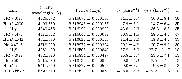
List of the absorption lines used to compute the orbital solution together with the adopted effective wavelengths. Column 3 gives the best-fit period value as deduced from the different RV data sets. The errors quoted were computed using the Wolfe, Horak & Storer algorithm. The primary and secondary apparent systemic velocities derived are respectively listed in Cols. 4 and 5. The last
column provides the number of RV points associated with each line data set
|
|
We selected eleven pure absorption lines in the spectrum of HD152248 to compute the orbital elements of the system. These lines were chosen according to the following criteria: the intensity of the line, the fact that they do not suffer a heavy blend with another neighbouring line at large RV separation phases (e.g. H ,
C IV
,
C IV
 5801-12) and the requirement that they should be free from pollution by any ISM lines (e.g. H
 )
or telluric lines (e.g. He I
)
or telluric lines (e.g. He I 7065). The selected lines are listed in Table 2. We measured the Doppler shifts by fitting two Gaussians at phases where the separation between the lines of both stars was sufficient. We then used the cross-correlation like method described in Rauw et al. (2000) to attempt to disentangle the blended lines. As HD152248 is an eclipsing binary, we used the light curve of PGB to achieve a rough first order correction of the relative line intensity at eclipsing phases. The observed lines are further affected by slight intensity and/or profile variations; we assumed, from our experience, that the errors on Doppler shifts measured in this way are about 2.5 times larger than the errors on the two-Gaussian fit results. For those phases where the lines were too heavily blended for the latter method to give reliable results, we adopted the RV obtained with a single Gaussian fit. We estimated, from the FWHM of the blend, that the accuracy on the line position in this latter case could be ten times lower than the one reached at large separation phases (i.e. with the two-Gaussian fit method). While computing the orbital solution, we thus attributed a relative weight of 1.0, 0.15 and 0.01 to the RVs respectively measured with the two-Gaussian fit, the cross-correlation like and the single Gaussian fit methods. Ruling out the single Gaussian fit points provides orbital parameters that are only marginally different.
We adopted the effective wavelengths for O stars listed in Table 2 to compute the barycentric RVs. These effective wavelengths are from Conti et al. (1977) below 5000 Å, and from Underhill (1994) above. As our spectra taken with different instruments cover different wavelength ranges, the number of RV points associated with the different lines is variable. We report this number in
Col. 6 of Table 2. The He I4471 line provides the largest data set with 47 RV points. These measurements are listed in Table 1.
Our orbital solution computation code is based on a modified version of the Wolfe, Horak & Storer algorithm (see Wolfe et al. 1967,
for the method; and Rauw et al. 2000, for the modifications implemented) and requires a previous knowledge of the orbital period to be run.
The best (i.e. with the smallest rms error) estimate of the period from the literature is
 days as given by ST96.
As the He I4471 RVs are the most numerous among our RV data, we first used this set to investigate the period value. For this purpose we applied the Lafler & Kinman method (Lafler & Kinman 1965) and the generalized spectrogramme Fourier technique (Heck et al. 1985). The results obtained with both methods lie within
5 10-4 days of the value of ST96, which is one order of magnitude smaller than the error estimated from the width of the peak in the periodogramme. We then iteratively ran our code, allowing for a differential correction of the orbital period. The convergence was reached in each case after a few iterations at most. This provides us with the period value which yields the orbital solution that best matches the observations (i.e. with the lowest rms residual) of the considered data set. Column 3 of Table 2 lists the period values obtained. Their weighted mean is
days as given by ST96.
As the He I4471 RVs are the most numerous among our RV data, we first used this set to investigate the period value. For this purpose we applied the Lafler & Kinman method (Lafler & Kinman 1965) and the generalized spectrogramme Fourier technique (Heck et al. 1985). The results obtained with both methods lie within
5 10-4 days of the value of ST96, which is one order of magnitude smaller than the error estimated from the width of the peak in the periodogramme. We then iteratively ran our code, allowing for a differential correction of the orbital period. The convergence was reached in each case after a few iterations at most. This provides us with the period value which yields the orbital solution that best matches the observations (i.e. with the lowest rms residual) of the considered data set. Column 3 of Table 2 lists the period values obtained. Their weighted mean is
 days, which is very close to the He I4471 value and contains both ST96 and Mayer et al. (1992) values within a
 interval. The very small uncertainty of the ST96 period determination results from the large time base of their IUE data set (
 5860 days) which is almost exactly four times ours. However, the HD152248 system is most probably undergoing an apsidal motion of a few degrees per year (see below and Mayer et al. 2001) and the large time base of ST96 could actually bias their period determination. In the following, we choose to adopt our mean value
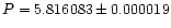
P = 5.816032 days for the orbital period.
5860 days) which is almost exactly four times ours. However, the HD152248 system is most probably undergoing an apsidal motion of a few degrees per year (see below and Mayer et al. 2001) and the large time base of ST96 could actually bias their period determination. In the following, we choose to adopt our mean value
P = 5.816032 days for the orbital period.
As a first step, we computed an orbital solution for each of the 11 absorption line data sets. Accounting for the error bars, the computed orbital elements do agree with each other, except for the apparent systemic velocities  and
and  (respectively associated with the primary and secondary star). Though the
and
values are in
acceptable agreement with each other for the same line (see Table 2), their values as deduced from the different lines are indeed significantly different. This illustrates the well-known effect that different lines might reflect different systemic velocities. This might stem from the fact that these lines are formed at different depths in the atmosphere and thus at different outward velocities, resulting in slightly different apparent systemic velocities.
(respectively associated with the primary and secondary star). Though the
and
values are in
acceptable agreement with each other for the same line (see Table 2), their values as deduced from the different lines are indeed significantly different. This illustrates the well-known effect that different lines might reflect different systemic velocities. This might stem from the fact that these lines are formed at different depths in the atmosphere and thus at different outward velocities, resulting in slightly different apparent systemic velocities.
In order to combine the RVs obtained from the different lines, we had to refer all the RV measurements to a ``zero systemic velocity'' reference frame. For this purpose, we simply subtracted the corresponding weighted mean between
and
from the individual RVs of the considered line. We then computed a weighted RV mean from all the RV data obtained at the same observing date.
These mean RVs in the zero systemic velocity reference frame are listed in Cols. 5 and 6 of Table 1.
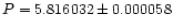
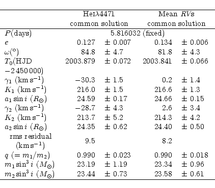
The computed orbital solutions from the He I4471 RV and the mean RV sets are both presented in Table 3. These two solutions are in excellent agreement with each other. Our way of combining the RVs from the different lines is further justified by the fact that the apparent systemic velocities computed from the mean data lie well within 1 of the zero velocity. We also tested the value of the period found by ST96. This does not affect the rms residual by more than a few tenths of kms-1 and the difference between the computed orbital elements is not significant.
Table 3:
Computed orbital solution for HD152248 using the RVs of the He I4471 absorption lines (left) or the mean RVs (right). T0 is the time of the periastron passage
|
|
![\begin{figure}
\par\includegraphics[height=7.5cm,width=7.9cm,clip]{MS10575f1.ps}\end{figure}](/articles/aa/full/2001/16/aa10575/Timg58.gif) |
Figure 1:
Radial velocity curve of the HD152248 binary system as computed from the He I4471 line plotted against the phase ( ). Different symbols refer to different instruments: ). Different symbols refer to different instruments:
 , ,
 , ,
 , ,
 .
Different sizes indicate different weights assigned to the data points in the computation of the orbital solution. Open symbols stand for the primary, while filled symbols indicate the secondary's RVs .
Different sizes indicate different weights assigned to the data points in the computation of the orbital solution. Open symbols stand for the primary, while filled symbols indicate the secondary's RVs |
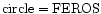
The He I4471 velocity curve is plotted in Fig. 1. This solution deduced from the optical wavelength domain is in good general agreement with the previous determination by ST96 from the UV domain. Our apparent systemic velocity is however 12kms-1 more positive than theirs. This difference might result from the zero velocity point in their cross-correlation method, but it is probable too that the optical and the UV domains reflect different apparent systemic velocities. Though the primary parameters from both our and their solution are very close, a more intriguing discrepancy is the difference between the mass ratios deduced. Indeed, our mass ratio (q=0.990) is much closer to unity than the ST96 value (q=0.941), and this manifests in the fact that our secondary component parameters K2 and  are larger. The minimal masses we derive are also larger than the values inferred by ST96 and PGB. Adopting the PGB value for the inclination
 yields absolute masses of
 and
and
 for the primary and the secondary respectively. We used Eggleton's formula (Eggleton 1983) to estimate the radii of the Roche lobe (RRL) for both components. Again assuming
yields respectively
for the primary and the secondary respectively. We used Eggleton's formula (Eggleton 1983) to estimate the radii of the Roche lobe (RRL) for both components. Again assuming
yields respectively
 and
and
 if we neglect the effect of the eccentricity (however see below). Thus if we adopt
 and
and
 ,
this result confirms the assertion of PGB that the system should not be undergoing a Roche lobe overflow (RLOF) mass transfer. However, Mayer et al. (2001) reported a lower value for the inclination (
,
this result confirms the assertion of PGB that the system should not be undergoing a Roche lobe overflow (RLOF) mass transfer. However, Mayer et al. (2001) reported a lower value for the inclination (
 )
and larger radii (
)
and larger radii (
 and
and
 ). In this latter case, the primary and secondary are respectively filling 72 and 91% of their Roche lobe volume at periastron. If these preliminary results of Mayer et al. (2001) for the radii are confirmed, we then expect the system to be very unstable near periastron passage and important mass transfer or mass loss could be initiated.
While recomputing the orbital solution from previously published RV data at different epochs in order to check the consistency of our method, we were led to suspect the presence of an apsidal motion within the binary system HD152248. In the following investigation, we considered three sets of data that are summarized in Table 4. We decided to ignore the complementary data obtained by HCB near
JD  440000 because their very poor phase coverage did not allow us to derive any significant constraint on the longitude of periastron.
Keeping the value of the orbital period and the eccentricity fixed at our new value, we have fitted the RV data from the literature. Table 4 lists the
440000 because their very poor phase coverage did not allow us to derive any significant constraint on the longitude of periastron.
Keeping the value of the orbital period and the eccentricity fixed at our new value, we have fitted the RV data from the literature. Table 4 lists the  values that provide the best fit to the various data sets. From these results, it is clear that the system is undergoing an apsidal motion. A simple linear regression yields a rate for the apsidal motion of about 3.4
 yr-1. A more detailed study by Mayer et al. (2001) based on new recent photometric results is currently underway. These authors independently discovered the presence of an apsidal motion in HD152248 and they estimate a period of 132 years, in acceptable agreement with our value.
Table 4:
Summary of the investigation we undertook to estimate the apsidal motion of the HD152248 system. Second to fourth columns list respectively the approximative mean JD in format JD
 ,
the time interval (expressed in days) and the number of RV points in the set. Column 5 reports the values of the angle of periastron passage ()
which provide the best fit. The last column lists the rms residual
between the best fit and the data
,
the time interval (expressed in days) and the number of RV points in the set. Column 5 reports the values of the angle of periastron passage ()
which provide the best fit. The last column lists the rms residual
between the best fit and the data
|
- 1.
Struve (1944); also described in HCB.
|
![\begin{figure}
\par\includegraphics[width=6.6cm,height=6.4cm,clip]{MS10575f2.ps}\end{figure}](/articles/aa/full/2001/16/aa10575/Timg72.gif) |
Figure 2:
Illustration of the variation of the He I4471 line strength. Note that the primary is on the blue side of the spectra at phases
 and 0.288 while it is on the red side of the spectra at the phases shown in the right panel. The depletion in the red wing of the spectrum at
 is the blue shifted secondary
 4481 line 4481 line |
![\begin{figure}
\par\includegraphics[width=7.5cm,height=6.3cm,clip]{MS10575f3.ps}\end{figure}](/articles/aa/full/2001/16/aa10575/Timg73.gif) |
Figure 3:
Primary to secondary ratios of the mean EWs of the He I lines in each quadrant. Downwards triangles = He I4026, circles = He I4471, diamonds = He I4713, squares = He I4922, upright triangles = He I5016 |
![\begin{figure}
\par\includegraphics[width=7.5cm,height=6.3cm,clip]{MS10575f4.ps}\end{figure}](/articles/aa/full/2001/16/aa10575/Timg74.gif) |
Figure 4:
Primary to secondary ratios of the mean EWs of the Balmer and the O III (upper panel) lines and of the He II (lower panel) lines in each quadrant. Upper panel: circles = H ,
diamonds = H ,
diamonds = H ,
upright triangles = O III 5592. Lower panel: squares = He II4200, circles = He II4542, downwards triangles = He II5411 ,
upright triangles = O III 5592. Lower panel: squares = He II4200, circles = He II4542, downwards triangles = He II5411 |
Up: HD 152248: Evidence for interaction
Copyright ESO 2001
![\begin{figure}
\par\includegraphics[height=7.5cm,width=7.9cm,clip]{MS10575f1.ps}\end{figure}](/articles/aa/full/2001/16/aa10575/img58.gif)
![\begin{figure}
\par\includegraphics[width=6.6cm,height=6.4cm,clip]{MS10575f2.ps}\end{figure}](/articles/aa/full/2001/16/aa10575/img72.gif)
![\begin{figure}
\par\includegraphics[width=7.5cm,height=6.3cm,clip]{MS10575f3.ps}\end{figure}](/articles/aa/full/2001/16/aa10575/img73.gif)
![\begin{figure}
\par\includegraphics[width=7.5cm,height=6.3cm,clip]{MS10575f4.ps}\end{figure}](/articles/aa/full/2001/16/aa10575/img74.gif)