| Issue |
A&A
Volume 709, May 2026
|
|
|---|---|---|
| Article Number | A264 | |
| Number of page(s) | 23 | |
| Section | Catalogs and data | |
| DOI | https://doi.org/10.1051/0004-6361/202557136 | |
| Published online | 22 May 2026 | |
S2D2: Small-scale, significant-substructure DBSCAN detection
II. Tracing episodes and gradients of star formation activity
1
Universidad Internacional de Valencia (VIU),
C/Pintor Sorolla 21,
46002
Valencia,
Spain
2
Univ. Grenoble Alpes, CNRS, IPAG,
38000
Grenoble,
France
3
Laboratoire d’astrophysique de Bordeaux, Univ. Bordeaux,
CNRS, B18N, all.e Geoffroy Saint-Hilaire,
33615
Pessac,
France
★ Corresponding author: This email address is being protected from spambots. You need JavaScript enabled to view it.
Received:
7
September
2025
Accepted:
12
March
2026
Abstract
Context. The spatial analysis of young stellar objects (YSOs) has proven very valuable to describe and analyse star-forming regions and to understand the star formation process.
Aims. This work aims to provide a homogeneous catalogue of small, significant substructures (henceforth NESTs) extracted from the spatial distribution of YSOs in a large, consistent sample of star-forming regions. The catalogue allowed us to explore the relevance of small-scale spatial substructure and discuss the interpretation of NESTs as tracers of star formation activity and remnants of the star formation process.
Methods. We applied our procedure to consistent catalogues of YSOs to obtain NESTs in a sample of star-forming regions. We applied a photometric classification scheme to obtain the evolutionary stage of YSOs and statistically explore the distribution of Class 0/I objects as a proxy of recent star formation activity.
Results. The region sample is diverse (in distance, size, structure, and global evolutionary stage), and we consequently found different structural properties and star formation histories. Most NESTs in regions with relevant recent star formation activity showed even higher levels of activity. Moreover, the proportion of NESTs with more activity than the region average increased with the global level of activity of the region. In approximately half of the regions, we also found significant spans in the evolutionary stages of the NESTs, consistently with gradients and episodes of star formation.
Conclusions. The combination of NESTs with a statistical exploration of the star formation history within each region provides robust and powerful insights into the star formation process. Our results support the role of NESTs as pristine remnants of star formation in highly active regions, highlighting the role of fragmentation. The combination of small structures with large-scale spatio-evolutionary patterns suggests hierarchical, prolonged, dynamic, and complex star formation scenarios.
Key words: methods: statistical / catalogs / open clusters and associations: general
© The Authors 2026
 Open Access article, published by EDP Sciences, under the terms of the Creative Commons Attribution License (https://creativecommons.org/licenses/by/4.0), which permits unrestricted use, distribution, and reproduction in any medium, provided the original work is properly cited.
This article is published in open access under the Subscribe to Open model. This email address is being protected from spambots. You need JavaScript enabled to view it. to support open access publication.
1 Introduction
Star formation (SF) is a complex, widespread phenomenon evolving at all spatial scales and timescales due to the rapid variation of diverse environmental factors. These include cloud density and dynamics, and, as SF proceeds, ionisation, heating, and stellar winds, which become particularly significant when massive stars form. Thus, star-forming regions are characterised by intricate spatial patterns across a wide range of scales both in the cloud component and the newly formed young stellar objects (YSOs). This work focuses on the spatial structure of the young object distribution, which shows a hierarchy of structures at scales from individual objects to clusters, complexes, and super-complexes.
Spatial analysis of YSOs is a powerful tool with which to study the formation and evolution of star-forming regions, particularly when combined with age or evolutionary estimates. YSOs can be classified in different evolutionary stages according to the infrared (IR) signatures linked to the accretion process. These are listed below:
Class 0/ I: less evolved objects, characterised by significant IR emission consistent with an accretion envelope with some emission from the protostar and a dense accretion disc in the Class I case.
Class II: YSOs in an intermediate evolutionary state, where the envelope has disappeared, showing photometric IR excess consistent with an accretion disc.
Class III: evolved YSOs, showing very low or no IR excess from an evolved, dissipated disc.
The spatial distribution of YSOs according to their classes or evolutionary stages has long been used to study the evolution of SF within a region (see, e.g. Sung et al. 2009, for the seminal study in NGC2264). The separation of areas of interest is key in such studies, and it is often related to the retrieval of relevant dense substructures. Methods of substructure retrieval often leave out the smaller spatial scales due to resolution limitations and the difficulty of separating them from spurious or random effects. This work focused specifically on small scales, complementing more traditional structure retrieval studies with their small-scale counterparts.
Joncour et al. 2018 (henceforth J18) analysed the small-scale substructures in the YSO distribution from Taurus, ensuring the significance by comparing the sample to complete spatial randomness (CSR). These retrieved significant substructures called nested elementary structures (NESTs), were on an intermediate spatial scale between ultra-wide pairs and loose groups, and their analysis proved very interesting. NESTs were typically associated with the molecular cloud, elongated, and aligned with the main gas filaments. Notably, approximately half of the NESTs (constituting less than 30% of all YSOs) contained 3/4 of all the Class 0/I objects. The work of J18 suggested that NESTs were the pristine remnants of the smallest collapsing gas structures.
In González et al. (2021a) (henceforth Paper I), we automated some steps in J18 for direct and consistent application in different regions, establishing the procedure small-scale, significant-substructure DBSCAN detection (S2D2). S2D2 is a robust procedure for the detection of small substructures, enforcing that the retrieved clusters (which we call NESTs as in J18) are significant compared to CSR. S2D2 reaches the smaller scales and avoids random fluctuations by requiring strict statistical density criteria for parameter selection, which implies that it is not sensitive to large-scale, moderate overdensities. We detail the procedure, highlighting its strengths and limitations, in Section 2.2.
We followed J18 and Paper I and applied S2D2 to a large sample of star-forming regions where all the members were determined homogeneously. We combined the NESTs with evolutionary stage estimates of YSOs to determine the range where NESTs can be considered the spatial imprints of recent SF and their potential as tracers of the SF history within a region.
This paper is structured as follows. In Section 2 we describe the samples and methods applied. We split the results over two sections: Section 3 contains aggregated results highlighting general trends, while in Section 4 we study the spatial distribution of NESTs. In Section 5 we contextualise and explore the role of NESTs as pristine remnants of SF and tracers of SF history, and finally, in Section 6, we summarise our results and conclusions. Additionally, in Appendix A we provide some useful tables (with the characteristics of all regions, acronyms used in this work, and a list of the online complementary material), and in Appendix B we detail the results for each of the regions analysed.
2 Method
In this section, we describe the sample and procedures applied to construct the catalogue of significant substructures that constitute the basis we used to compare SF amongst various regions. Both the use of samples homogeneously obtained and a robust, common method of retrieval are important to ensure that the comparison of substructures retrieved across regions is as fair and unbiased as possible.
2.1 Star-forming region sample: MYStIX and SFiNCs programmes
The MYStIX programme (Feigelson et al. 2013) was an observational project designed to obtain the young stellar population of a sample of massive star-forming regions within 4 kpc of the Sun. The programme complemented near-IR data with X-ray observations (allowing for the detection of a larger number of objects) and curated a list of member candidates for each region while trying to minimise contamination. The final sample of probable members of each region was obtained using Bayesian inference (Broos et al. 2013) by combining data from Spitzer IRAC (Fazio et al. 2004), 2MASS (Skrutskie et al. 2006), UKIDSS (Lawrence et al. 2007), and Chandra (Weisskopf et al. 2000). Known OB stars from the literature were also added to the catalogues.
The SFiNCs programme (Getman et al. 2017) subsequently aimed to extend and complement the MYStIX sample and focused specifically on smaller, nearby regions. The observational advantages of closer regions allowed for a simpler membership and evolutionary stage determination, but the project was designed and implemented to maintain sample consistency between programmes.
These projects provided the community with homogeneous and comparable catalogues of young stellar members of all the studied regions (Broos et al. 2013; Povich et al. 2013, and Getman et al. 2017), suited to spatial structure studies. Despite their age, the MYStIX and SFiNCs catalogues are still relevant and represent some of the most complete samples of YSO candidates in their respective regions, due to the inclusion of selected X-ray sources. We verified this by comparing the samples with the SPICY catalogue, a large YSO candidate catalogue based on IR-excess containing more than 100 000 sources (Kuhn et al. 2021). We only found matches in approximately one-third of the regions. In all them, the number of SPICY members is less than half the number of MYStIX and SFiNCs candidates, and most of them are already in the MYStIX/SFiNCs sample. K14 applied a parametric mixture model of isothermal ellipsoids to detect the substructures present in each of the MYStIX regions, and the same methodology was later extended to the SFiNCs sample (Getman et al. 2018b, henceforth G18). These sub-clusters were used to describe the regions, and their physical, kinematical, and age characteristics were estimated in later studies (Kuhn et al. 2015, Kuhn et al. 2019, and Getman et al. 2018a). In this work, we applied S2D2 to retrieve the NESTs in the MYStIX and SFiNCs catalogues, providing a complementary perspective to those of from the K14 and G18 analyses.
2.2 S2D2: NEST retrieval and calibration
We now briefly describe the S2D2 procedure used to retrieve the NESTs that constitute our catalogue, as described in Appendix A. We refer the reader to Paper I for an extensive description of the method, its calibration and behaviour in both synthetic and observed control regions, and the available public implementations1.
S2D2 selects the parameters of DBSCAN (Ester et al. 1996) using statistical criteria to detect small-scale structures that are significant above random expectation. DBSCAN is a well-known density-based algorithm focused on two parameters: the scale, ε, which defines a local neighbourhood for each star, and a minimum number of neighbours, Nmin. Together, ε and Nmin define a nominal density requirement:  . DBSCAN does not force all the elements of the sample into clusters, nor does it impose a specific number of structures, and it can detect structures of any shape. However, its parameter choice limits its output to a specific density, and it can be weak to gradual density variations, which may lead to spurious separation or the merging of structures.
Appendix C in J18 compares DBSCAN with other clustering methods, but many variations have appeared to improve it in terms of efficiency, parameter dependence, and quality of clusters (Bushra & Yi 2021). Given that S2D2 specifically addresses parameter selection and that the scope of the method covers datasets of moderate size, the most relevant category is the quality of clusters, particularly in datasets characterised by large density ranges such as star-forming regions. Despite being beyond the single-scale focus of this work, the multi-scale variations of OPTICS and HDBSCAN, which probe a range in ε and produce a hierarchy of substructures, are relevant in an SF context. Cánovas et al. (2019) found comparable results for the three algorithms in ρ Ophiuchi, but HDBSCAN is often favoured over OPTICS due to computational speed and because cluster selection is direct. In addition to making it possible to consider datasets with density variations, the high sensitivity of HDBSCAN justified its selection by Hunt & Reffert (2021) to retrieve clusters from Gaia data. The disadvantage of HDB-SCAN is a false positive problem which forces a curation a posteriori of the structures. In some of the tests from Bushra & Yi (2021), HDBSCAN retrieved a larger number of clusters than expected, pointing to the splitting of single structures that did not appear for DBSCAN. The work of Hunt & Reffert (2021) also showed very good precision for DBSCAN, with low levels of false positives. The counterpart showed decreased sensitivity, with DBSCAN failing to detect some structures. The false positive issue is particularly problematic on small scales, which are severely affected by random fluctuations. This justifies the choice of DBSCAN for our work, even at the cost of completeness.
The procedure of S2D2 is to select the parameters of DBSCAN to ensure a theoretical level of significance compared to a random distribution. The retrieval scale, ε, was chosen using the smallest scale that shows a transition from an excess to a defect of stars in the region with respect to random expectation, as shown by the one-point correlation function Ψ (OPCF, described in Joncour et al. 2017). We calculated Nmin using the probability density function of the nth nearest neighbour (J18) to guarantee that the structures retrieved have a significance above 99.75 % with regard to random expectation. The density of the CSR control distribution ρCSR representative of the complete region was calculated using the expression described in Paper I.
In Paper I, we calibrated S2D2 with 90 synthetic regions (10 random realisations of 9 different spatial distributions). The regions followed distributions representing clusters with global fractal substructure (fractal-box models) and large-scale concentrations (radial or Plummer distributions) with various parameters, including fractal and radial approximations of CSR. We found low levels of spurious detection in CSR, and the number of NESTs (as well as the fraction of objects within them) increased with the level of substructure or concentration. In substructured, fractal distributions we retrieved small NESTs all over the region, with a limited fraction of objects within the NESTs. In concentrated distributions we often found groups of NESTs corresponding to a single large-scale structure and comprising a substantial proportion of YSOs.
We also applied S2D2 to observed regions, beyond the boxfractal and radial paradigm to evaluate the performance of the algorithm in real star-forming regions. We analysed an updated sample of Taurus, with ∼ 30% more members than J18, and obtained a similar number, position and size of NESTs. This supported the reliability of the automations in the process and the robustness of the structures retrieved by S2D2. In the Carina region, also using the sample of MYStIX in this work, we recovered NESTs in the areas corresponding to the known clusters Trumpler 15, 14, and 16 and the Treasure Chest, but not Bochum 11, in the south. NESTs were inside or close to the central ellipsoids of the structures retrieved by K14, and all the members of NESTs in Carina were members of K14 clusters. We also found that NESTs were always in zones of high clustering tendencies according to INDICATE (a density-based statistical index that quantifies the degree of spatial clustering or association of each object Buckner et al. 2019). A substantial fraction of structures from K14 in Carina did not have NEST counterparts. Some of them were in zones with significant INDICATE clustering tendencies and known clusters, and they are possibly large structures with densities that S2D2 is insensitive to. Others, however, have low-density values and clustering tendencies and may be background density fluctuations.
To further ensure that NEST retrieval is not affected by binaries and chance alignments, we merged all the stars that are closer than a specified threshold. We chose an angular threshold of 2″, similar to the resolution of the Spitzer IRAC and 2MASS observations, instead of a physical one, because the distance between regions is significant and a limit valid for the farthest regions can excessively degrade the closest ones. This implies that in the farthest regions, we cannot sample spatial scales as small as those in the closer ones.
Paper I analysed the results of S2D2, finding low levels of spurious detection and coherent behaviour in a variety of situations, and supporting our confidence in NESTs. The appearance of groups of NESTs, while out of the initial scope, was consistent along both synthetic and real regions, and provides a way to trace significant large-scale concentrations. However, we need to keep in mind that NESTs cannot produce a complete description of the entire substructure within a region, as S2D2 is insensitive to structures of lower relative density.
2.3 Evolutionary state of YSOs, NESTs, and regions
This section describes the procedure we used to derive evolutionary stage estimates for each NEST. We used NGC2264 (a region long studied with spatial analysis of objects of different evolutionary stages by, e.g. Sung et al. 2009, Rapson et al. 2014, Venuti et al. 2018, and Nony et al. 2021) as a benchmark to evaluate the validity and performance of our approach. In our tests, we find that our procedure provides a consistent global picture for NGC2264 even when we use different samples or evolutionary stage estimates. Detailed results of these tests can be accessed as online complementary material, as indicated in Appendix A.
2.3.1 Evolutionary stage estimates of YSOs
All the objects in the catalogues from K14 and G18 were selected as young stellar members of the regions, based on photometric, statistical, and spatial criteria. For a fraction of these members, estimates of their evolutionary stage were provided. While both relied on IR photometry, the method to estimate the evolutionary stage of YSOs in the MYStIX regions differs from the one applied for SFiNCs. The evolutionary stage classification of YSOs in MYStIX regions was performed by Povich et al. (2013) and relied on spectral-energy-distribution (SED) fitting to calculate the α IR spectral slope index. For the closer, less crowded SFiNCs regions, Getman et al. (2017) provided a simpler classification of members with and without disks based on IR excess.
For the sake of consistency and homogeneity, we reclassified all the objects using the method by Gutermuth et al. (2009) (henceforth G09), which was also applied by Rapson et al. (2014) to NGC2264. Buckner et al. (2019) found that within the objects in common, Rapson et al. (2014) had more unambiguously classified sources than K14.
We briefly describe the classification scheme from G09, which used Spitzer and 2MASS data to retrieve YSOs based on their IR excess. The method works in three steps (phases I, II, and III, following the terminology in G09), and each of them applies some cuts in colour-colour and colour-magnitude diagrams to distinguish YSOs from non-stellar contaminants. Phase I uses the Spitzer-IRAC four-band data to characterise Class 0/I and Class II objects separating them from broad-band AGNs, and shock/PAH-emission sources. In Phase II, objects without IRAC data of sufficient quality are characterised using dereddened 2MASS HJKs photometry. Phase III performs a final check of the catalogue to retrieve some additional Class 0/I objects with Spitzer-MIPS 24-micron data. It also allows for the distinction of Class III from transition-disc objects and more evolved stars and confirm the YSOs detected in previous phases.
The MYStIX and SFINCs datasets do not have MIPS data, and we obtained a very low number of coincidences when crossmatching the YSO catalogue with MIPSGAL sources. Thus, we did not include this information as it would not statistically improve the procedure and could introduce differences in the classifications between regions. We note, however, that without the information from MIPS, we cannot perform phase III, and objects classified as Class III cannot be distinguished from main-sequence stars. All the sources in this work were already selected as young stellar members of the regions by K14 and G18, so we assume that they are Class III objects.
Some objects in the catalogues do not have photometric data of sufficient quality to provide a reliable classification, and others are classified as non-stellar (e.g. AGN, PAH, etc.) in the different phases. All these are discarded from our evolutionary analysis, while the rest will be kept to statistically evaluate the evolutionary status of the region and its NESTs. Each selected object is labelled Class 0/I, Class II, or Class III. This classification, along with the NEST membership on each object, is provided as complementary material.
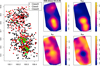 |
Fig. 1 Spatial distribution and relative-risk maps for NGC2264. Left: spatial distribution of objects in NGC2264. Dots represent each source in the complete sample, coloured according to the evolutionary stage classification described in Section 2.3.1 (green for Class 0/I, red for Class II, black for Class III, and empty for unclassified and non-stellar objects). Right: four-panel composite showcasing the associated densities and relative-risk maps. Top left: KDE estimate corresponding to the classified sub-sample in the left panel. Top right: relative-risk maps of Class 0/I objects. Bottom panels: relative-risk maps of Class II and Class III objects. |
2.3.2 Kernel density estimate and relative risk
The proportion of YSOs in each class provides a global average estimate of the evolutionary status within a region. Comparing these ratios in different zones can shed light on the history of SF within a region, accounting for the spatial distribution of the objects of different classes.
While the probable members of MYStIX and SFiNCs provide a large, complete, and homogeneously obtained independent sample of YSOs, an evolutionary stage classification of the full sample is impossible, as many members were detected in X-rays and lack IR photometry of sufficient quality. This prevented us from simply counting the elements of each class, and we instead propose a statistical approach in the following analysis. We illustrate this process for region NGC2264 in Figure 1, which is composed of five panels organised in two rows. In the online complementary materials described in Appendix A, we provide additional tests in this region. The large left panel of Figure 1 shows the spatial distribution of all the sources in the region, coloured according to their class (calculated as described in Section 2.3.1). Green dots stand for Class 0/I, red dots for Class II, black dots for Class III, and empty circles for objects classified as non-stellar or unclassified.
First, we applied a fixed-bandwidth Gaussian kernel density estimate (KDE) for the spatial distribution of YSOs. Since the bandwidth choice problem is related to the bias/variance tradeoff problem, a universally optimal parameter does not exist. As S2D2 computes the relevant small scale of NEST retrieval for each region, ε, we chose the value h = 10 ∙ ε to smooth the distribution. This allowed us to keep the bandwidth scale related to that of the NESTs and consistently use the same approach for all regions.
Our approach is based on the spatial analysis of a sub-sample of the members classified as stellar in each region. To obtain robust results, this stellar sub-sample needs to be representative of the complete population. We flagged all regions where the stellar sub-sample includes less than 50 % of the members as unreliable and excluded them from further evolutionary analysis. We also visually compared the KDE intensity maps from the complete and stellar sample to ensure that both distributions were similar. The top left panel on the right side of Figure 1 shows the KDE of the stellar sample for NGC2264.
Once the stellar sub-sample’s density was deemed representative of the spatial distribution of all members, we used the same bandwidth to compute a non-parametric estimate of relative risk. Relative risk is an exploratory spatial analysis technique widely used in the epidemiological domain (see, e.g. Diggle 2003, and references therein) to evaluate the spatial variation of a case of interest such as occurrences of a disease. Relative risk weights the intensity of the case of interest with that of a control (in our case, the stellar sub-sample). This translates into a quotient of KDEs, providing a continuous and smoothed approach to the ratio of the case of interest within a region. The values of relative risk can be interpreted as the probability of an object at a specific location belonging to the case of interest. In this work, we used the less evolved objects (Class 0/I) as the case of interest, but this approach can be applied to any category.
The top right and bottom panels of the right side of Figure 1 show the relative-risk maps of Class 0/I (left), Class II (middle), and Class III objects in NGC2264. The relative risk maps expose the distribution of objects, showing a complex SF history for this region consistent with the view provided by numerous previous studies (such as Sung et al. 2009; González & Alfaro 2017, Venuti et al. 2018, and Nony et al. 2021). Class 0/I objects are concentrated in the Cone sub-cluster area towards the south, particularly in the Cone (C) and Spikes areas (where we use the common terminology for the sub-regions initially proposed by Sung et al. 2009). The largest proportions of Class II objects are in the Spike sub-region north of Cone-C and the northern S-Mon sub-region. Finally, Class III objects are spread all over, but they constitute the majority of sources in the periphery, comprising the halo and part of S-Mon.
We used R (R Core Team 2023) to apply the relativerisk implementations in spatstat (Baddeley & Turner 2005 and Baddeley et al. 2015), including standard edge corrections and an estimate of the standard error.
2.3.3 NEST evolutionary estimates and significance
We estimated the evolutionary state of each NEST from the values of the relative-risk maps at its position. We took the position of a NEST as the centroid of the minimum spanning ellipsoid of its members, as J18 showed that NESTs are generally small and elongated. The relative risk of Class 0/I objects in each NEST, fC0/I, is a proxy of its recent activity level and evolutionary stage and consistently traces the SF history within each region.
We note that a straightforward interpretation of the relative risk value suffers from similar issues as ratios obtained from direct counting, where low numbers undermine the reliability of an observed ratio, fC0/I. We recommend caution, particularly in areas of low YSO density. This work focused on NESTs, which are by definition of high density and mitigate this problem, but it should be kept in mind when interpreting the complete relative risk distribution. The consistent application of relative-risk maps to different regions in this work will prove that they are a powerful, valuable tool with which to explore the SF history of a region.
The standard-error estimation map for the relative risk was calculated using the variances of the estimated intensities of the analysed point pattern. While this estimate is valuable, and we provide it for each NEST, it is tied solely to the specific analysed pattern, without controlling for significance with regard to a spatial random distribution. We followed the philosophy of the S2D2 procedure and determined a global significance level for the fC0/I values in each region using a random distribution of the class labels.
We redistributed the labels randomly within the stellar subsample and recomputed the corresponding relative-risk maps using the same parameters. For each re-sampling we obtain a distribution of relative-risk values, r, with the average and standard deviations: f̄, σf. We performed this procedure 100 times, obtaining 100 relative-risk maps: fi, i = 1,..., 100. The mean values of their averages and deviations, f̄i, σfi, i = 1,..., 100, were used as the global average and dispersion control values for each region. The value of f̄C0/I is very close to the ratio of Class 0/I objects within a region,  , where NC0/I is the number of Class 0/I objects and Nclass the number of classified objects:
  . The average dispersion, σfC0/I, is a conservative estimate of the uncertainty, as it is at least a factor of two larger than the mean of the relative-risk standard error map in all of the regions in this work.
Given that all sources were extracted from observations with the same instruments, differences in distance are associated with the spatial resolution. We expect an impact on the size of the observed regions, on ε, on the scale of NEST retrieval, and on the values of fC0/I. We explored these biases in the online complementary material described in Appendix A and limited comparisons of fC0/I in NESTs to their host region, which is expected to be fair and independent of distance. A NEST has a significantly high (resp. low) fC0/I value in relation to its host region if  (resp.
  )..
)..
3 Results
The combination of MYStIX and SFiNCs has 39 regions, but we excluded a region with very few members: LDN1251B. In this section, we discuss the results for the sample of 38 regions.
3.1 General structure and characteristics
The main structural characteristics of the regions and spatial analysis results are summarised in Table 1. A complete table with all the individual values is available online and described in Appendix A. The general characteristics of regions portray a very heterogeneous sample, with values of several physical features spanning more than an order of magnitude. Distances range from 235 to 3600 pc, and the number of objects, N ∈ [63, 2790]. Nmerged ∈ [63, 2708], was obtained after merging objects within 2″ to account for multiples and chance alignments that could lead to spurious NEST retrieval. We also calculated a typical size, R, for each region as the radius of the convex hull of its members, which ranges from 0.61 to 21.1 pc. Given the distance range and its associated resolution limit, we studied its influence on some key parameters and results on the online supplementary material separately.
After applying S2D2, we found 254 NESTs, which are not homogeneously distributed amongst regions. The maximum number of NESTs retrieved in a region was reached in Eagle, with 23 NESTs; while in NGC1333 and ONC-Flank N, we did not retrieve any significant structure. We verified the compactness of the NESTs using the relative density. The ratio between the nominal retrieval density of NESTs, ρnom, and that of the region, ρCSR :  . ρrel, is larger than ten for all regions and reached a maximum value of 37.74, confirming the compactness of NESTs in all regions. As for the retrieval characteristics of S2D2, Nmin stays stable, with low values between four and five; and the differences between regions reflect the physical size scale, ε, which ranges from 3.45 to 39.34 kAU and has a relative nominal density of 10.55 ≤ ρrel ≤ 37.74.
As a first global approach to analysing the structure of each region, we calculated the Q parameter, introduced by Cartwright & Whitworth (2004). The Q parameter is a numerical index to evaluate whether regions display substructure or single concentrations or are indistinguishable from CSR within a box-fractal and radial model paradigm. Although limited in terms of discerning capability, it can broadly distinguish sub-structured, clumpy distributions (Q ⪅ 0.7) from large-scale concentrations (Q ⪆ 0.87) and CSR (Q ≈ 0.8). We refer the reader to Parker 2018 and to the appendix in Paper I for a more detailed discussion on the power and limitations of and alternatives to the Q parameter.
Figure 2 shows the relative density values, ρrei, against Q, with the marginal distributions as density profiles in their respective axes. The global structure traced by the parameter Q indicates significant diversity across regions, with 0.43 ≤ Q ≤ 1.01. The distribution of Q is spread out and peaks at 0.85, displaying a shoulder at around 0.65. In Figure 2, we hatched the background of the regions with Q ≤ 0.7 (resp. Q ≥ 0.87), showing clear signs of structure (resp. central concentration) in the box-fractal and radial paradigm. It is noteworthy that those thresholds are close to the quartiles of the Q distribution, meaning that approximately half of the regions are in a range consistent with CSR and low structure levels. As cautioned in Paper I, as Q was calibrated in the box-fractal and radial paradigm, realistic complex regions with substructures can present values of Q consistent with CSR and need to be studied with particular care.
The distribution of ρrel is mainly concentrated between 10 and 20, peaking at around 15. We note three regions with ρrel > 30: NGC1333, ONC-Flank N, and SFO2. The high-density requirement along with values of Q ~ 0.8 in NGC1333 and ONC-Flank N are consistent with the CSR simulations from Paper I, supporting the validity of the lack of significant structure detection in these regions. SFO2 has Q = 0.88, pointing to a large-scale concentration traced by a single NEST.
Other characteristics shown in Table 1 such as the fraction of stars in NESTs fNEST and  , which represents the population of the largest NEST in each region relative to Nmin, also span ample ranges, and their distribution supports the notion that we have a varied sample with significantly different levels of substructure and concentration.
Summary statistics of structural characteristics of regions.
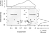 |
Fig. 2 Relative density of NESTs compared to that of the region’s ρrel versus Q structural parameter. The marginal distributions are shown as density profiles on their respective axes. The hatched zones indicate values of Q corresponding unequivocally to sub-structured (Q ⪅ 0.7) and concentrated (Q ⪆ 0.87) distributions. |
3.2 Evolutionary stage classification: Regimes of recent activity
We used the ratio of less evolved objects,  , as a global indicator of recent SF activity and, as explained in Section 2.3, conservatively flagged the classification of all regions where the ratio of classified objects is fclass < 0.5. Regions flagged for classification are Orion, M17, NGC6334, RCW38, NGC1893, and Trifid. These are excluded from all discussions regarding recent SF activity.
The global statistics of the 32 remaining regions involving the evolutionary stage classification, namely fclass and the estimates for the relative-risk average and standard deviation for each class, {f̄A, σfA}, A ∈ C0/I, CII, CIII}, are summarised in Table 2. The values in Table 2 show that C0/I objects are the minority in all regions. This can be explained by the difference in average lifetimes for each kind of objects: 0.5 Myr for Class 0/I and 2 Myr for Class II (Evans et al. 2009). With a constant SF rate, the ratio of C0/I objects fC0/I steadily decreases and drops below 0.5 after 1 Myr and 0.25 at 2 Myr. The ratio fCII increases until 2 Myr and decreases from 2.5 Myr onward, as the oldest Class II objects transition to Class III ones. After only 4.5 Myr, in this toy model the ratios are fC0/I = 0.1, fCII = 0.4, and fCIII = 0.5.
We separated the regions in the sample into three different categories according to fC0/I. This separation into regimes of recent activity allowed us to simplify our discussion by organising all the information derived from our different analyses. We considered using age-based criteria, but there are large differences between estimates by various authors, as well as age variations within regions that prevent an objective, consistent separation (see, e.g. Mendigutía et al. 2022). Despite the limitations of fC0/I this criterion can be applied homogeneously to all sampled regions. The regions are categorised as follows:
High recent activity (HRA): eight regions with f̄C0/I ≥ 0.135
Intermediate recent activity (IRA): 16 regions with 0.04 < f̄C0/I ≤ 0.135
Low recent activity (LRA): eight regions with f̄C0/I ≤ 0.04
The chosen boundaries are quartiles of the f̄C0/I distribution of regions with reliable classification, producing a simple and compatible split with qualitative notions of high-intermediate-low activity, but other choices may also be valid. The purpose of defining these regimes is to functionally and broadly categorise regions consistently and facilitate further analyses.
Figure 3 summarises the results of the global evolutionary stage YSO classification for all regions with a reliable classification. The fractions of objects of different classes are shown as stacked bars, and the regions are ordered in decreasing order according to the value of f̄C0/I. The colours represent the recent regime of SF activity in each region, and the shade of each colour represents each class. Darker bars represent f̄C0/I, medium bars f̄CII, and the lightest colour represents the fraction f̄CII.
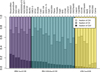 |
Fig. 3 Stacked bar diagram representing the fraction of stellar objects of each evolutionary state in each (not flagged) region, ordered by Class 0/I fraction. The colour of the bars represents the regime attributed to each region: purple for HRA regions, green for IRA regions, and yellow for LRA regions, as explained in the main text. The intensity of each bar represents the different classes of objects in each region, with darker shades representing less evolved objects. |
Summary statistics of the classification results in the region sample with accepted classifications.
3.3 Evolutionary stage of NESTs
In this section we describe how we used the proportion of Class 0/I objects to estimate the evolutionary stage of NESTs and explore the SF history of each star-forming region. As described in Section 2.3, we statistically estimated the fraction of Class 0/I objects within a NEST, fC0/I, and compared it to the average of the region, f̄C0/I. We then classified NESTs as high-activity, average, or low-activity based on whether fC0/I is significantly larger than, consistent with, or significantly lower than f̄C0/I.
The results for all NESTs grouped by regime are shown in Table 3. Globally, 34% of NESTs trace particularly active areas within a region, 59% show an average level of activity, and only 7% have significantly lower activity. In HRA regions, with a global activity level of fC0/I > 13.5%, the majority of NESTs show even higher activity: we find 77% of them are high-activity NESTs, 18% are average, and 5% (2 out of 44) are low-activity. In IRA regions, 29% of NESTs are high-activity, 60% average, and 11% low-activity. In LRA regions, we only find 5% are high activity NESTs, while the other 95% are average. A Pearson χ2 test of independence provides a p value of 0.0005, confirming with a high degree of confidence that the distribution of NEST recent activity varies with the SF regime of its host region.
The main results seen in Table 3 are that NESTs do not typically trace areas significantly less active than the region average (7%), and that the proportion of high-activity NESTS decreases with the global recent activity level. Table 3 also points to significant variations in the activity of NESTs within a region. Indeed, the span of fC0/I of NESTs within each region,  , ranges from 0 to 0.37. In 12 regions, we find it to be significant, with ∆fNEST > σfC0/I. These account for half of the regions where ∆ fNEST can be calculated (24 regions with reliable evolutionary classification and more than one NEST).
We explored the recent history of SF through the evolutionary stage estimates of NESTs in Figure 4, which has four panels. Each panel represents regions within each regime, in decreasing order of the maximum value of fC0/I for NESTs, max fC0/I. The top panel shows HRA regions, the two middle panels correspond to IRA regions, and the bottom panel shows LRA regions. Each region is represented by a bar with height corresponding to the average value ratio of the region (f̄C0/I) and is coloured according to its regime (purple for HRA, green for IRA, and yellow for LRA). The significance thresholds, f̄C0/I ± σfC0/I, in each region are represented by dashed black lines. Black points show the Class 0/I ratio for each NEST, fC0/I, with its standard deviation as error bars. NESTs are ordered decreasingly by their fC0/I values.
Globally, Figure 4 shows that in most regions there are NESTs with a larger than average fC0/I. Indeed, that is the case for ∼76% of regions with NESTs (23 out of 30 regions with reliable classification and NESTs), and in almost half of them (14 out of 30) there are NESTs significantly more active than average. The ratio of more active NESTs also decreases with the global level of activity.
The top panel of Figure 4 shows the results for all HRA regions with NESTs, ordered by max fC0/I. In all HRA regions with NESTs, at least some of them have a larger than average fC0/I. This difference is significant in most of them, meaning that they host high-activity NESTs. The only exception is Serpens Main, where one NEST is very close to the significance threshold but does not cross it. We only found low-activity NESTs in IRAS20050+2720 and NGC2068-2071, both regions known as sub-structured regions hosting two clusters, with all the low-activity NESTs grouped together.
We found significant values of the span of NESTs ∆ fNEST > σfC0/I in six out of seven regions with NESTs. The outsider is again Serpens Main, with  . Figure 4 shows both smooth patterns and sudden drops in the fC0/I distribution of NESTs in HRA regions. The spatial distribution of NESTS will determine whether these patterns can be attributed to activity gradients, separate episodes of SF, or different sub-clusters. The general results of such an analysis are described in the next section (and detailed for each region in Appendix B).
The middle panels of Figure 4 show the results for all 14 IRA regions. Four IRA regions have a significant NEST activity span, ∆ fNEST > σfC0/I, and six regions have a single NEST. Most regions (13/16) have at least one NEST with a larger fC0/I than average, and it is significant in seven of them. As with HRA regions, we find high-activity NESTs in all regions with ∆fNEST > σfC0/I, accompanied by average and/or low-activity NESTs. In the rest of the IRA regions with more than one NEST, all have similar levels of activity, which is generally average. The exceptions are IC348, where all the NESTs are low-activity, and GGD12-15, where all NESTs are high-activity.
Finally, the bottom panel of Figure 4 shows the results for the eight IRA regions. Here, the global ratio of Class 0/I objects is low, and the dispersion, σfC0/I, is of the order of the estimate, f̄C0/I. Only Cep OB3B shows a significant activity span and hosts NESTs with significantly high activity levels. The activity of the rest of the NESTs in LRA regions is consistently average. Our results show NESTs often trace particularly active areas within a region, with higher activity NESTs being more frequent in regions with significant levels of recent activity.
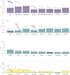 |
Fig. 4 Bar plots display the average fraction of C0/I objects in each region, with dotted black lines indicating the limits for categorizing NESTs as high-activity or low activity, that is |

Classification of NESTs according to their evolutionary stage estimated from fC0/I, grouped by the recent activity regime of the host region.
4 Spatial distribution of NESTs
In this section, we show results related to the spatial distribution of NESTs within each region in combination with the evolutionary stage estimates. Individual detailed results for all regions are shown in Appendix B, with additional online complementary materials available.
4.1 Comparison with K14 and G18
We naturally compared our results with the works K14 and G18, which used the same region catalogues. In the supplementary materials, described in Appendix A, we also compare our work with other clustering methods, namely the MST method shown in Getman et al. (2018b) and HDBSCAN. K14 and G18 fitted a mixture model with an unclustered component and isothermal ellipsoids of varying densities and sizes. The best fit was selected with the Akaike information criterion (AIC), and each ellipsoidal component of the final configuration is considered a substructure. The main conclusions of the tests performed in Paper I for Carina and described in Section 2.2 remain, even when expanding the sample of regions: NESTs trace the densest parts within each region and are usually close to the core ellipsoids from K14 and G18, and NESTs do not detect some of the structures from K14 and G18. There are arguments supporting the notion that some of these structures can be spurious as the AIC does not take into account significance; modeling a single irregular structure may require several ellipsoidal components that do not forcefully correspond to a proper substructure, and in their solutions there is always at least a cluster. On the other hand, S2D2 is not sensitive to halos or other real, large-scale secondary substructures that do not reach its strict density requirements. Paper I showed that for complex regions where a single comparison density is not appropriate, separating the region before applying S2D2 could lead to the detection of more structures.
Regarding the global number of objects in structures, 65% of the sample is attributed to a proper substructure in K14 and G18 (i.e., excluding their field component, X, and stars with unclear membership), while only 11% of all objects are in NESTs. Only 4% of stars in NESTs (101 objects) belong to the field/unclear component, either because they are part of the NESTs that partially overlap with proper structures or because they are small, compact, isolated NESTs. We note that the majority of these objects both in NESTs and field/unclear components from K14 and G18 are in regions such as M17, Eagle, or RCW38, which have several K14 and G18 substructures that overlap in core-halo or multiple clump configurations and have high ratios of objects of unclear membership.
In Figure 5, we compare the general characteristics of the structures from each method. We used common estimates that can be calculated for any clustering solution and considered the differences between regions. In the top plot, the histogram compares the sizes of the structures, calculated as the equivalent radius of its reported members in kilo astronomical units. The distribution of sizes is clearly different, with the NEST distribution very skewed towards low values and the distribution of clusters from K14 and G18 much more spread out. The situation is reversed for the relative density-distribution histogram of the retrieved clusters,  , where the density of a structure is given by its number of members and the area of its convex hull,
  , and ρCSR is the CSR characteristic density of its host region. From the middle panel of Figure 5 it is clear that the distribution of the ρrel of NESTs is much more spread out and peaks at higher values than that of clusters from K14 and G18, which are very skewed towards low values.
The bottom panel of Figure 5 compares the distribution of fC0/I in NESTs and structures from K14 and G18 for all regions with NESTs and a reliable classification. The figure shows the average fC0/I in each region as a grey bar, and horizontal dotted lines mark the limits f̄C0/I ± σfC0/I. On top of the bars, Figure 5 shows the median value of the fC0/I relative-risk map within the convex hull of NESTs (red dots) and clusters K14 and G18 (black dots), with an error bar of the corresponding colour spanning the first and third quartiles. The aggregated results from Figure 5 are consistent with those for individual NESTs shown in Figure 4, showing a trend between the activity of NESTs relative to the average and the global level of activity of a region. Structures from K14 and G18 do not show such a clear pattern, and being larger, their distribution of fC0/I is also more spread out. The median fC0I in NESTs is similar to or larger than fC0I in structures from K14 and G18 in all of the HRA regions and most IRA and LRA regions, with the exceptions of Cep A, Eagle, and IC348, where NESTs have lower median values. For IC348 and Cepheus A, Figure 4 shows values of fC0/I consistent with or significantly lower than the region average, and for Eagle, only two out of 23 NESTs have significantly high activity, so their high fC0/I values are not expected to appear in the part of the distribution shown.
The comparison with K14 and G18 confirms that S2D2 consistently retrieves a small-scale, very dense substructure characterised by high activity levels, at least for the less evolved regions. We note again that NESTs leave behind less compact structures, which could be part of a more complete description of star-forming regions.
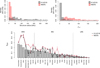 |
Fig. 5 Comparison of structures from K14 and G18. Top left: histogram of the size of NESTs (red) and the structures from K14 and G18 in kilo astronomical units. Top Right: histogram of relative average density and the structures from K14 and G18. Bottom: grey bars show the average ratio, f̄C0/I, in each region, with small horizontal dotted lines showing the limits f̄C0/I ± σfC0/I. Red (resp. black) dots show the median values of fC0/I from the relative-risk maps in the area occupied by the convex hull of NESTs (resp. structures from K14 and G18), with error bars representing the first and third quartiles. Solid red (resp. black) lines join the median values of fC0/I for NESTs (resp. K14 and G18) to help compare the values. Finally, vertical lines separate the HRA, IRA, and LRA regimes. |
4.2 HRA regions
The YSO distribution in most HRA regions shows one or more large-scale concentrations traced by NESTs. There are six regions with significant ∆fNEST, which allowed us to trace gradients in the SF activity of large-scale structures (Serpens South, DR21, Mon R2), different sub-clusters (IRAS200050+2720, NGC2068-2071), and feedback effects (RCW120).
The HRA regions with gradients are particularly interesting, as they form elongated patterns that also overlap with dense gas structures. Promising preliminary work (González et al. 2021b) explored the relationships between NESTs and the gas distribution using Herschel (Pilbratt 2010) data of surveys focusing on SF (such as HOBYS, Motte et al. 2010), and we intend to investigate it further in the future. Figure 6 shows maps of two HRA regions showing NEST chains: DR21 and Serpens South. Each panel displays the YSOs within a region as grey asterisks and the centroids of NESTs as coloured symbols. Circles indicate NESTs of average activity, triangles high-activity NESTs, and inverted triangles low-activity NESTs. The colour of each NEST corresponds to its value of fC0/I according to the colour bar to the right. Contours show the relative risk map of Class 0/I YSOs. Red contours correspond to the threshold values f̄C0/I ± σfC0/I, separating the areas of significantly high (solid line) or low activity (dashed line). We show analogous plots for all regions, along with a detailed analysis in Appendix B and larger versions of the maps as complementary materials, as described in Appendix A.
Both DR21 and Serpens South display a large group of NESTs in the centre of the region following an elongated pattern and with significantly high activity (fNEST ⪆ 0.4), while the more peripheral NESTs have significantly lower fC0/I values, indicating an outwardly decreasing activity ratio. Region DR21 has a richer substructure, displaying several sub-chains along the main concentration.
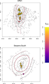 |
Fig. 6 Maps of selected HRA regions with NESTs. Grey dots represent the YSOs in the area, and coloured markers show the position of NESTs. Symbols indicate whether the activity of NESTs is significantly different (triangles for larger and inverted triangles for lower activity) or consistent with the average (circles). The colour-scale shows the ratio of Class 0/I objects assigned to each NEST. Contours show each region’s relative-risk map values, and red contours mark the threshold boundaries, f̄C0/I ± σfC0/I, separating areas with values different from the average control distribution for each region (solid red contour for the upper limit and dashed red contour for the lower limit). |
4.3 IRA regions
In IRA regions, we can distinguish two basic patterns in the spatial distributions of YSOs and, consequently, NESTs. We show representative examples of both in Figure 7. Each panel shows a map of a region, displaying the YSOs as grey asterisks and the centroids of NESTs as coloured symbols, with the same code as in Figure 6.
The first group comprises IRA regions showing clear signs of substructure traced by distinct groups of NESTs. These regions have larger sizes (R ⪆ 4 pc), most of them also contain high-activity NESTs with high fC0/I values, and their NEST population shows a significant span of activity: ∆ fNEST. The top panel of Figure 6 shows such a pattern in the Rosette nebula, where we find several separate groups of NESTs whose values of f0/I globally increase towards the south. The largest population is the southernmost one, which shows a similar configuration to that of HRA regions discussed in the previous section: an elongated configuration of high-activity NESTs with an outwardly decreasing gradient of recent activity.
The second pattern in IRA regions corresponds to smaller fields (R ⪅ 3 pc) showing a much simpler history. Their distribution of YSOs is consistent with some level of spatial concentration, and we find a single NEST or group of NESTs, all with similar recent SF activity, which is usually higher than average (significantly so in approximately half of the cases). An example of this is shown in the bottom panel of Figure 7. Only NGC6357, where we trace three distinct sub-clusters from NESTs with similar average activity levels, does not fit any of the patterns we just described.
4.4 LRA regions
Structurally, LRA regions are varied. We find spatially distinct groups of NESTs in half of the regions, mainly corresponding to known clusters and large-scale structures. Figure 8 shows the maps of LRA regions, Cep OB 3b and NGC2362, with the same symbols as the previous Figures 6 and 7. LRA regions are characterised by their low global ratio of Class 0/I objects, indicating low levels of recent star formation, and the dispersion σfC0/I is of the order of fC0/I. For these regions individually, the ratio of Class 0/I-Class II objects could be a more informative indicator, but in this work, we kept the fC0/I for the sake of general consistency in the comparison with other regions.
The recent SF history we traced in LRA regions is simple: we only found NESTs with activity levels other than average in one region out of eight, that is, Cep OB3b. In this region, shown in the top panel of Figure 8, we find a pair of high-activity NESTs at the centre of the field, while NESTs towards the east and west have average activity. In LRA regions, recent star formation plays a lesser role, and the retrieved significant structure can be associated with older SF events that dominate the YSO distribution. An example of such a situation is NGC2362, shown in the bottom panel of Figure 8.
5 Discussion
In this section, we discuss the role of NESTs in the study of SF, focusing on their interpretation as remnants of the SF process. Choices in the implementation of S2D2 were oriented towards robustness in terms of structure retrieval (see the online complementary material described in Appendix A for a detailed comparison with other methods of structure extraction), but as any spatial technique applied in 2D, it can be affected by projection effects. Projection effects are ultimately a lack of information that can be extremely relevant, depending on the unknown underlying situation. Specific studies show that the trends detected by INDICATE are robust to both evolutionary and projection effects (Buckner et al. 2024, Buckner et al. 2022, and Blaylock-Squibbs & Parker 2024). In Paper I we verified that S2D2 is consistent with INDICATE, and the retrieved NESTs are all in areas of strong clustering tendencies. We note, however, that specific further analyses (which are out of the scope of this work) are needed to verify that the most clustered stars, including those that would be in NESTs, are preserved in projection.
5.1 NESTs as imprints of SF
Both observations (e.g. Sanchez et al. 2024; Buckner et al. 2020, and references therein) and simulations (e.g. Pelkonen et al. 2024; Verliat et al. 2022,and references therein) support a higher level of substructure for the spatial distribution of less evolved YSOs. Younger stars are typically grouped towards the densest gas, while the older ones show a more homogeneous distribution. The procedure S2D2, by construction, recovers the denser substructures that we expect from younger objects.
The potential of NESTs as tracers of recent SF is also substantiated by SF scenarios where small structures of young objects appear as a consequence of fragmentation. A recent semi-analytical model for hierarchical fragmentation by Thomasson et al. (2024) predicted structures compatible with the size and number of objects in NESTs found in Taurus by J18, as well as with the cloud fragments retrieved in NGC2264 (Thomasson et al. 2022). The size distribution of NESTs (top left panel of Figure 5) is very skewed towards low sizes and has median radius of 10 kAU, which is compatible with fragmentation imprints. As J18 proposed for Taurus, the smaller NESTs could be the product of the fragmentation of a single molecular core, while the larger ones may trace clusters of cores.
The work of Vázquez-Semadeni et al. (2025) compares the current state of the global-hierarchical-collapse (GHC) model with turbulent-support (TS) scenarios. Both are hierarchical models comprising turbulence and gravity, but the roles and effects of these processes are fundamentally different. The main difference between the two views is the overall state of the molecular cloud. In the GHC model there is a global contraction and fragmentation, while in the TS model turbulence produces an almost hydrostatic cloud. While there are not specific predictions regarding small scales, the GHC model expects a gravitational fragmentation cascade that can obtain sizes consistent with NESTs (Vázquez-Semadeni et al. 2019). We also lack information at smaller scales for the TS, but in the related turbulent core SF model from McKee & Tan (2003) for massive SF, where fragmentation of cores has low theoretical probabilities, primordial NESTs are not expected.
We remind the reader that, as described in Section 3.2, we used estimates of the ratio fC0/I to determine of the level of recent activity for both NESTs and regions and separated regions into categories of high, intermediate, and low recent activity (HRA, IRA, and LRA) according to their global ratio of Class 0/I objects. Our general results show that while it is not uncommon to find highly active NESTs (⪆30%), low-activity NESTs are rare as they constitute 7% of the total. Moreover, the evolutionary distribution of NESTs within a region is dependent on its global regime of activity: the less globally evolved a region, the greater the chances of finding high-activity NESTs within it. In HRA regions, most NESTs show high activity levels, and most HRA regions contain at least one high-activity NEST. Both the overall ratios of high-activity NESTs and regions containing them decline with the global level of activity.
If we consider NESTs as potential pristine remnants of SF, their persistence is key, as the general picture emerging from both observations and simulations for the early evolution of young clusters is very dynamic. While we lack specific analysis at small scales, simulations show that structures often appear, interact, dissolve, merge, and split, while new stars still form during the embedded phases (see, e.g. Guszejnov et al. 2022, and Dobbs et al. 2022). After a few megayears, when the cloud starts dispersing, structures typically expand, although structure remains can persist. Associations seem particularly stable, retaining significant levels of substructure despite their expansion (Cantat-Gaudin & Casamiquela 2024).
Miret-Roig et al. (2024) found a discrepancy of ∼5 Myr between the isochronal and dynamical ages in six young clusters, attributed to the embedded phase delaying the onset of pure dynamical evolution. These timescales are larger than the average expected lifetimes of Class 0/I and II objects, supporting limited effects of dynamical evolution in our samples, at least for those without large Class III ratios.
In active regions such as DR21, MonR2, or Serpens, we found elongated structures of high-activity NESTs overlapping with dense gas. This spatial configuration is similar to some found in IRA regions (southern group of NESTs in Rosette) or without a reliable classification (e.g. NGC1893 or NGC6334) and in Taurus by J18. In Taurus, NESTs were also aligned with the gas elongated structures, as would be expected for the remnants of the fragmentation of filaments. Large groups of NESTs overlapping hubs or ridges of dense gas (such as NGC2264, Orion, M17, Flame, or GDD 12-15) are also common.
The spatial distribution of NESTs matches the evolutionary morphological path proposed by K14, in particular the predominance of string-like structures of NESTs associated with gas in highly active regions. K14 proposed that linear sub-cluster chains inherited their structure directly from gas filaments and evolved towards more concentrated morphologies, such as those that would be traced by a NEST (or a group of them). The spatial distribution of NESTs is also compatible with the high-mass formation scenario outlined in Motte et al. (2018), where ridges and hubs undergo a global collapse which increases the masses of both the ridge/hub and its forming protostars.
In scenarios where large structures of YSOs form by the assembly of smaller substructures (as suggested by simulations by e.g. Dobbs et al. 2022 and Vázquez-Semadeni et al. 2017, NESTs could either detect the large-scale structures themselves or some lasting remains of the individual components, depending on the level of dynamical mixing. An analysis of kinematical data could help constrain the dynamical status of NESTs and their members.
Our results support that NESTs, at least those highly active in HRA regions, are the pristine imprints of SF as suggested by J18. The interpretation of low-activity NESTs is less straightforward, as it depends on the level of interactions within each region. Some can be infertile remnants of earlier SF, while others could have assembled later on.
5.2 Tracing SF history within a region
We show that relative-risk maps provide a powerful, visual approach to the global SF history within a region. The interpretation of maps should be done carefully, considering the specifics of each sample. In this work, we applied this technique on a large scale and focused mainly on NESTs, particularly compact ones, to maximise the underlying density support. We believe carefully exploring the complete maps can be worthwhile, particularly for structures traced by single NESTs (e.g. Eagle, Sh2-106, Cep A, Cep C, SFO2, RCW36).
Not all structures traced by NESTs are high-activity ones, nor are they necessarily associated with relative-risk peaks or dense gas substructures. Indeed, we even find groups of low-activity (IRAS20050+2720, NGC2078-2071, NGC2264, Rosette) or average NESTs (Eagle, Rosette, W40) in HRA and IRA regions. These groups could be remnants of earlier SF depleting the local gas reservoirs. However, being generally evolved regions, they may also have suffered a relevant amount of dynamical evolution, and their interpretation needs to consider all the specific aspects in each region.
Large groups of NESTs may also display significant differences in activity, allowing us to trace evolutionary SF patterns. We find outward gradients continuously traced by NESTs, often associated with highly active, globally collapsing clouds (e.g. DR21, Mon R2, and Serpens South), where large clusters are potentially assembling. Similar outward gradients have been observed in several young clusters (see the recent summary by Stahler 2024 and references therein). Getman et al. (2018a) also found gradients in substructures retrieved from the MYStIX-SFiNCs samples, and our work supports their findings.
While such evolutionary gradients can be due to projection effects of sequential SF (Maaskant et al. 2011), they can also form naturally in some SF scenarios. In the GHC, they are associated with accretion at all scales: the older stars formed in the filaments are displaced and end up distributed over larger areas than their younger counterparts, forming inside the clump (Vázquez-Semadeni et al. 2017). In a TS paradigm, age gradients only form in simulations when gradual SF is included (Farias et al. 2019). Stahler (2024) proposed outwards diffusion of stars forming in the centre due to overcrowding that creates a halo-like structure called mantle. The gradient appears as new stars form in the densest part and different structures, such as open clusters, would be produced by the disruption of the mantles. In the slingshot mechanism (Stutz & Gould 2016), the magnetic field produces a transverse wave oscillating along a filament with active SF. Newborn objects follow the oscillations and inherit the transverse velocity as they decouple from the gas. Some of these scenarios overlap the eight options that Getman et al. (2014) grouped in three blocks. The first one involves more recent SF in the centre of the structure, due to the gas density gradient, acceleration of the SF rate with time, or an age stratification similar to the one reported for high-mass stars. The second option involves older stars moving outward and basically includes scenarios related to the dynamical evolution of the YSOs. These include drift or relaxation from super-virial or sub-virial initial configurations, and the effects of initial substructure as older clusters expand more. In the final alternative, younger stars move inward, either as infalling filaments or subcluster mergers. While we cannot discard the presence of other effects, the appearance of groups of NESTs tracing large-scale substructures aligns our results with the infalling filament and sub-cluster merger scenarios.
We also find large-scale evolutionary patterns consistent with sequential SF in regions such as NGC2264, Rosette, or with major feedback effects, as in RCW120. In approximately 1/3 of the regions, we find spatially distinct groups of NESTs often coincident with known clusters. This is the case for larger regions (R ≥ 4 pc), where NESTs outline the most significant overdensities. These structures generally have significantly different levels of recent activity, principally in HRA and LRA regions, making NESTs effective tracers of different SF episodes within each region. The variety and complexity of the patterns that we find are supported by the spatio-kinematical analysis from Gaia data reporting the appearance of large-scale spatio-temporal patterns in associations (Kerr et al. 2024 and Ratzenböck et al. 2023). Their results point to both the continuous formation of low-mass clusters and episodes of heightened SF with separations of several megayears.
This work, which only includes spatial and evolutionary analysis of YSO candidates, can solely provide a partial view on SF, a very complex and widespread phenomenon that involves several processes that are extremely hard to quantify. We expect such an event to adopt different forms depending on the specific conditions, so studies including kinematics as well as characteristics of the maternal cloud are required to obtain a more complete picture. Despite these limitations, our results favour a hierarchical scenario comprising fragmentation such as the GHC. This would be compatible with the structure we find at all spatial scales and the scenarios in Getman et al. (2014) explicitly including large-scale substructures, such as infalling filaments or sub-cluster mergers.
6 Summary and conclusions
We created a catalogue of NESTs retrieved by S2D2 in a homogeneous sample of YSOs of 38 star-forming regions. The regions vary in size, distance, population, activity, and structure. The properties of the NESTs retrieved within them are also heterogeneous. We find a total of 254 NESTs in 36 regions, and none in the remaining two (NGC1333 and ONCFlankN), which show other indicators of consistency with CSR. We do not find significant global patterns of the number of NESTs, Q parameter, fraction of objects within NESTs, or relative maximum population of NESTs with the regime of recent SF.
We estimated the evolutionary stage of the YSOs in each region using IR photometry and separated the regions with reliable classification in three recent activity regimes depending on their observed ratio of Class 0/I objects, fC0/I. We calculated the relative risk of Class 0/I objects (which can be interpreted as the probability of finding an object of Class 0/I at a given position), and propose a statistical indicator of the evolutionary state of the NESTs within each region. Based on this, we determined whether the level of recent activity in each NEST is significantly higher than, lower than, or consistent with the average of the region.
Our results support the idea that NESTs can trace the preferential sites of SF in regions with high recent SF activity. There, NESTs tend to show high levels of activity, overlap dense gas structures, and are often arranged in elongated patterns or groups consistent with pristine remnants of the fragmentation of filaments and cluster assembly process. The probability of retrieving high-activity NESTs decreases with the global level of recent SF, and the probability of dynamical processing of the traced spatial structures increases.
The spatial distribution of NESTs themselves provides useful insights into the most significant large-scale structures. In approximately half of the regions, we find a significant span on the level of recent activity of NESTs. This is often due to distinct spatial structures that display different activity levels, effectively tracing separate clusters and episodes of SF. We were also able to detect activity gradients inside groups of NESTs that could be attributed to sequential SF, hierarchical collapse, stellar mantle drifts, or feedback effects.
Our work balances the power of relative-risk maps and the high significance of NESTs to trace the remnants of SF and discern different patterns of SF history. The variety of spatial structures and evolutionary patterns we obtain favours hierarchical multi-scale models comprising fragmentation, such as the GHC. We note, however, that our analyses are limited to the spatial and evolutionary studies, so these conclusions must be supported by additional evidence, notably kinematics and the behaviour of the gas. Preliminary work shows promising results (González et al. 2021b) regarding the systematic separation and analysis of groups of NESTs in combination with the study of gas within a region.
Data availability
Tables with the characteristics of regions are available at the CDS via https://cdsarc.cds.unistra.fr/viz-bin/cat/J/A+A/709/A264.
Online complementary materials are available online in Zenodo (https://doi.org/10.5281/zenodo.18955037). They are described in detail in Appendix A, and include tables of each region with the members of NESTs and photometrical classification.
Acknowledgements
We thank the anonymous referee, whose comments and suggestions improved this manuscript. This work acknowledges funding from European Union’s Horizon 2020 research and innovation program under grant agreement no. 687528 (STARFORMMAPPER) and the European Research Council (ERC) via the ERC Synergy Grant ECOGAL (grant 855130). This project has received funding from the Spanish Agencia Estatal de Investigación (MICIU/AEI/10.13039/501100011033) and FEDER, EU through project TACOS (PID2023-146635NA-I00) as well as the French Agence Nationale de la Recherche (ANR) through the project COSMHIC (ANR-20-CE31-0009).
References
- Allen, T. S., Gutermuth, R. A., Kryukova, E., et al. 2012, ApJ, 750, 125 [Google Scholar]
- Alzate, J. A., Bruzual, G., Kounkel, M., et al. 2023, MNRAS, 523, 4821 [Google Scholar]
- Baddeley, A., & Turner, R. 2005, J. Statist. Softw., 12, 1 [Google Scholar]
- Baddeley, A., Rubak, E., & Turner, R. 2015, Spatial Point Patterns: Methodology and Applications with R (London: Chapman and Hall/CRC Press) [Google Scholar]
- Bally, J., Chia, Z., Ginsburg, A., et al. 2022, ApJ, 924, 50 [NASA ADS] [CrossRef] [Google Scholar]
- Beccari, G., Petr-Gotzens, M. G., Boffin, H. M. J., et al. 2017, A&A, 604, A22 [NASA ADS] [CrossRef] [EDP Sciences] [Google Scholar]
- Bešlić, I., Coudé, S., Lis, D. C., et al. 2024, A&A, 684, A212 [NASA ADS] [CrossRef] [EDP Sciences] [Google Scholar]
- Blaylock-Squibbs, G. A., & Parker, R. J. 2024, MNRAS, 528, 7477 [Google Scholar]
- Bonne, L., Schneider, N., García, P., et al. 2022, ApJ, 935, 171 [NASA ADS] [CrossRef] [Google Scholar]
- Bonne, L., Bontemps, S., Schneider, N., et al. 2023, ApJ, 951, 39 [CrossRef] [Google Scholar]
- Broos, P. S., Getman, K. V., Povich, M. S., et al. 2013, ApJS, 209, 32 [NASA ADS] [CrossRef] [Google Scholar]
- Buckner, A. S. M., Khorrami, Z., Khalaj, P., et al. 2019, A&A, 622, A184 [NASA ADS] [CrossRef] [EDP Sciences] [Google Scholar]
- Buckner, A. S. M., Khorrami, Z., González, M., et al. 2020, A&A, 636, A80 [NASA ADS] [CrossRef] [EDP Sciences] [Google Scholar]
- Buckner, A. S. M., Liow, K. Y., Dobbs, C. L., Naylor, T., & Rieder, S. 2022, MNRAS, 514, 4087 [Google Scholar]
- Buckner, A. S. M., Naylor, T., Dobbs, C. L., Rieder, S., & Bending, T. J. R. 2024, MNRAS, 527, 5448 [Google Scholar]
- Bushra, A. A., & Yi, G. 2021, IEEE Access, 9, 87918 [Google Scholar]
- Cánovas, H., Cantero, C., Cieza, L., et al. 2019, A&A, 626, A80 [NASA ADS] [CrossRef] [EDP Sciences] [Google Scholar]
- Cantat-Gaudin, T., & Casamiquela, L. 2024, New A Rev., 99, 101696 [CrossRef] [Google Scholar]
- Cartwright, A., & Whitworth, A. P. 2004, MNRAS, 348, 589 [Google Scholar]
- Chung, E. J., Lee, C. W., Kim, S., et al. 2024, ApJ, 970, 122 [Google Scholar]
- Damian, B., Jose, J., Samal, M. R., et al. 2021, MNRAS, 504, 2557 [NASA ADS] [CrossRef] [Google Scholar]
- Diggle, P. J. 2003, Statistical Analysis of Spatial Point Patterns (Wiley and Sons) [Google Scholar]
- Dobbs, C. L., Bending, T. J. R., Pettitt, A. R., Buckner, A. S. M., & Bate, M. R. 2022, MNRAS, 517, 675 [NASA ADS] [CrossRef] [Google Scholar]
- Eiroa, C., Djupvik, A. A., & Casali, M. M. 2008, in Handbook of Star Forming Regions, Volume II, 5, ed. B. Reipurth, 693 [Google Scholar]
- Ester, M., Kriegel, H.-P., Sander, J., & Xu, X. 1996, in Proceedings of the Second International Conference on Knowledge Discovery and Data Mining, KDD’96 (AAAI Press), 226 [Google Scholar]
- Evans, II, N. J., Dunham, M. M., Jørgensen, J. K., et al. 2009, ApJS, 181, 321 [Google Scholar]
- Farias, J. P., Tan, J. C., & Chatterjee, S. 2019, MNRAS, 483, 4999 [NASA ADS] [CrossRef] [Google Scholar]
- Fazio, G. G., Hora, J. L., Allen, L. E., et al. 2004, ApJS, 154, 10 [Google Scholar]
- Feigelson, E. D., Townsley, L. K., Broos, P. S., et al. 2013, ApJS, 209, 26 [Google Scholar]
- Fukui, Y., Torii, K., Ohama, A., et al. 2016, ApJ, 820, 26 [Google Scholar]
- Getman, K. V., Feigelson, E. D., & Kuhn, M. A. 2014, ApJ, 787, 109 [NASA ADS] [CrossRef] [Google Scholar]
- Getman, K. V., Broos, P. S., Kuhn, M. A., et al. 2017, ApJS, 229, 28 [Google Scholar]
- Getman, K. V., Feigelson, E. D., Kuhn, M. A., et al. 2018a, MNRAS, 476, 1213 [Google Scholar]
- Getman, K. V., Kuhn, M. A., Feigelson, E. D., et al. 2018b, MNRAS, 477, 298 [Google Scholar]
- González, M., & Alfaro, E. J. 2017, MNRAS, 465, 1889 [Google Scholar]
- González, M., Joncour, I., Buckner, A. S. M., et al. 2021a, A&A, 647, A14 [Google Scholar]
- González, M., Joncour, I., & Moraux, E. 2021b, in The 20.5th Cambridge Workshop on Cool Stars, Stellar Systems, and the Sun, 321 [Google Scholar]
- Günther, H. M., Wolk, S. J., Spitzbart, B., et al. 2012, AJ, 144, 101 [Google Scholar]
- Guszejnov, D., Markey, C., Offner, S. S. R., et al. 2022, MNRAS, 515, 167 [NASA ADS] [CrossRef] [Google Scholar]
- Gutermuth, R. A., Megeath, S. T., Myers, P. C., et al. 2009, ApJS, 184, 18 [Google Scholar]
- Gutermuth, R. A., Pipher, J. L., Megeath, S. T., et al. 2011, ApJ, 739, 84 [Google Scholar]
- Hacar, A., Tafalla, M., & Alves, J. 2017, A&A, 606, A123 [NASA ADS] [CrossRef] [EDP Sciences] [Google Scholar]
- Hennemann, M., Motte, F., Bontemps, S., et al. 2010, A&A, 518, L84 [NASA ADS] [CrossRef] [EDP Sciences] [Google Scholar]
- Hennemann, M., Motte, F., Schneider, N., et al. 2012, A&A, 543, L3 [NASA ADS] [CrossRef] [EDP Sciences] [Google Scholar]
- Hunt, E. L., & Reffert, S. 2021, A&A, 646, A104 [NASA ADS] [CrossRef] [EDP Sciences] [Google Scholar]
- Itrich, D., Testi, L., Beccari, G., et al. 2024, A&A, 685, A100 [NASA ADS] [CrossRef] [EDP Sciences] [Google Scholar]
- Jia, D., Yu, H., Shao, Z., & Li, L. 2024, AJ, 168, 79 [Google Scholar]
- Joncour, I., Duchêne, G., & Moraux, E. 2017, A&A, 599, A14 [NASA ADS] [CrossRef] [EDP Sciences] [Google Scholar]
- Joncour, I., Duchêne, G., Moraux, E., & Motte, F. 2018, A&A, 620, A27 [NASA ADS] [CrossRef] [EDP Sciences] [Google Scholar]
- Karnath, N., Prchlik, J. J., Gutermuth, R. A., et al. 2019, ApJ, 871, 46 [NASA ADS] [CrossRef] [Google Scholar]
- Kerr, R., Kraus, A. L., Krolikowski, D., Bouma, L. G., & Farias, J. P. 2024, ApJ, 975, 99 [Google Scholar]
- Kirk, H., Johnstone, D., Di Francesco, J., et al. 2016, ApJ, 821, 98 [Google Scholar]
- Kounkel, M., Stassun, K. G., Covey, K., & Hartmann, L. 2022, MNRAS, 517, 161 [NASA ADS] [CrossRef] [Google Scholar]
- Kuhn, M. A., Feigelson, E. D., Getman, K. V., et al. 2014, ApJ, 787, 107 [Google Scholar]
- Kuhn, M. A., Feigelson, E. D., Getman, K. V., et al. 2015, ApJ, 812, 131 [NASA ADS] [CrossRef] [Google Scholar]
- Kuhn, M. A., Hillenbrand, L. A., Sills, A., Feigelson, E. D., & Getman, K. V. 2019, ApJ, 870, 32 [CrossRef] [Google Scholar]
- Kuhn, M. A., de Souza, R. S., Krone-Martins, A., et al. 2021, ApJS, 254, 33 [NASA ADS] [CrossRef] [Google Scholar]
- Kuhn, M. A., Hillenbrand, L. A., Feigelson, E. D., et al. 2022, ApJ, 937, 46 [NASA ADS] [CrossRef] [Google Scholar]
- Lawrence, A., Warren, S. J., Almaini, O., et al. 2007, MNRAS, 379, 1599 [Google Scholar]
- Luhman, K. L., Esplin, T. L., & Loutrel, N. P. 2016, ApJ, 827, 52 [Google Scholar]
- Luisi, M., Anderson, L. D., Schneider, N., et al. 2021, Sci. Advances, 7, eabe9511 [Google Scholar]
- Maaskant, K. M., Bik, A., Waters, L. B. F. M., et al. 2011, A&A, 531, A27 [Google Scholar]
- McKee, C. F., & Tan, J. C. 2003, ApJ, 585, 850 [Google Scholar]
- Mendigutía, I., Solano, E., Vioque, M., et al. 2022, A&A, 664, A66 [NASA ADS] [CrossRef] [EDP Sciences] [Google Scholar]
- Mintz, A., Hora, J. L., & Winston, E. 2021, AJ, 162, 236 [NASA ADS] [CrossRef] [Google Scholar]
- Miret-Roig, N., Alves, J., Barrado, D., et al. 2024, Nat. Astron., 8, 216 [Google Scholar]
- Motte, F., Zavagno, A., Bontemps, S., et al. 2010, A&A, 518, L77 [CrossRef] [EDP Sciences] [Google Scholar]
- Motte, F., Bontemps, S., & Louvet, F. 2018, ARA&A, 56, 41 [NASA ADS] [CrossRef] [Google Scholar]
- Mužić, K., Almendros-Abad, V., Bouy, H., et al. 2022, A&A, 668, A19 [NASA ADS] [CrossRef] [EDP Sciences] [Google Scholar]
- Nony, T., Robitaille, J. F., Motte, F., et al. 2021, A&A, 645, A94 [NASA ADS] [CrossRef] [EDP Sciences] [Google Scholar]
- Ordenes-Huanca, C., Zoccali, M., Bayo, A., et al. 2024, MNRAS, 533, 841 [Google Scholar]
- Parker, R. J. 2018, MNRAS, 476, 617 [Google Scholar]
- Pelkonen, V. M., Miret-Roig, N., & Padoan, P. 2024, A&A, 683, A165 [NASA ADS] [CrossRef] [EDP Sciences] [Google Scholar]
- Peterson, D. E., & Megeath, S. T. 2008, in Handbook of Star Forming Regions, Volume I, 4, ed. B. Reipurth, 590 [Google Scholar]
- Pilbratt, G. 2010, in JENAM 2010, Joint European and National Astronomy Meeting, 149 [Google Scholar]
- Povich, M. S., Kuhn, M. A., Getman, K. V., et al. 2013, ApJS, 209, 31 [NASA ADS] [CrossRef] [Google Scholar]
- R Core Team 2023, R: A Language and Environment for Statistical Computing, R Foundation for Statistical Computing, Vienna, Austria [Google Scholar]
- Rapson, V. A., Pipher, J. L., Gutermuth, R. A., et al. 2014, ApJ, 794, 124 [Google Scholar]
- Ratzenböck, S., Großschedl, J. E., Alves, J., et al. 2023, A&A, 678, A71 [NASA ADS] [CrossRef] [EDP Sciences] [Google Scholar]
- Russeil, D., Schneider, N., Anderson, L. D., et al. 2013, A&A, 554, A42 [NASA ADS] [CrossRef] [EDP Sciences] [Google Scholar]
- Sadaghiani, M., Sánchez-Monge, Á., Schilke, P., et al. 2020, A&A, 635, A2 [NASA ADS] [CrossRef] [EDP Sciences] [Google Scholar]
- Sanchez, N., Nespoli, E., Gonzalez, M., & Climent, J. B. 2024, A&A, 688, A224 [Google Scholar]
- Schneider, N., Csengeri, T., Bontemps, S., et al. 2010, A&A, 520, A49 [CrossRef] [EDP Sciences] [Google Scholar]
- Skrutskie, M. F., Cutri, R. M., Stiening, R., et al. 2006, AJ, 131, 1163 [NASA ADS] [CrossRef] [Google Scholar]
- Stahler, S. W. 2024, MNRAS, 529, 4512 [Google Scholar]
- Stoop, M., Kaper, L., de Koter, A., et al. 2023, A&A, 670, A108 [NASA ADS] [CrossRef] [EDP Sciences] [Google Scholar]
- Stoop, M., Derkink, A., Kaper, L., et al. 2024, A&A, 681, A21 [NASA ADS] [CrossRef] [EDP Sciences] [Google Scholar]
- Stutz, A. M., & Gould, A. 2016, A&A, 590, A2 [NASA ADS] [CrossRef] [EDP Sciences] [Google Scholar]
- Sugitani, K., Tamura, M., & Ogura, K. 1995, ApJ, 455, L39 [Google Scholar]
- Sun, J., Gutermuth, R. A., Wang, H., Zhang, S., & Long, M. 2022, MNRAS, 516, 5258 [Google Scholar]
- Sung, H., Stauffer, J. R., & Bessell, M. S. 2009, AJ, 138, 1116 [Google Scholar]
- Thomasson, B., Joncour, I., Moraux, E., et al. 2022, A&A, 665, A119 [NASA ADS] [CrossRef] [EDP Sciences] [Google Scholar]
- Thomasson, B., Joncour, I., Moraux, E., et al. 2024, A&A, 689, A133 [NASA ADS] [CrossRef] [EDP Sciences] [Google Scholar]
- Tigé, J., Motte, F., Russeil, D., et al. 2017, A&A, 602, A77 [Google Scholar]
- Torii, K., Hattori, Y., Hasegawa, K., et al. 2017, ApJ, 835, 142 [NASA ADS] [CrossRef] [Google Scholar]
- Treviño-Morales, S. P., Fuente, A., Sánchez-Monge, Á., et al. 2019, A&A, 629, A81 [NASA ADS] [CrossRef] [EDP Sciences] [Google Scholar]
- Vázquez-Semadeni, E., González-Samaniego, A., & Colín, P. 2017, MNRAS, 467, 1313 [NASA ADS] [Google Scholar]
- Vázquez-Semadeni, E., Palau, A., Ballesteros-Paredes, J., Gómez, G. C., & Zamora-Avilés, M. 2019, MNRAS, 490, 3061 [Google Scholar]
- Vázquez-Semadeni, E., Palau, A., Gómez, G. C., et al. 2025, MNRAS [arXiv:2408.10406] [Google Scholar]
- Venuti, L., Prisinzano, L., Sacco, G. G., et al. 2018, A&A, 609, A10 [NASA ADS] [CrossRef] [EDP Sciences] [Google Scholar]
- Verliat, A., Hennebelle, P., González, M., Lee, Y.-N., & Geen, S. 2022, A&A, 663, A6 [NASA ADS] [CrossRef] [EDP Sciences] [Google Scholar]
- Weisskopf, M. C., Tananbaum, H. D., Van Speybroeck, L. P., & O’Dell, S. L. 2000, SPIE Conf. Ser., 4012, 2 [Google Scholar]
- Wolk, S. J., Winston, E., Bourke, T. L., et al. 2010, ApJ, 715, 671 [Google Scholar]
- Wright, N. J., & Parker, R. J. 2019, MNRAS, 489, 2694 [Google Scholar]
- Young, K. E., Young, C. H., Lai, S.-P., Dunham, M. M., & II, N. J. E. 2015, AJ, 150, 40 [Google Scholar]
Appendix A Useful lists and tables
Appendix A.1 Acronyms
We start by describing the acronyms used in this work, in alphabetical order
AIC: Akaike information criterion. Criterion used in K14 and G18 to select the number of clusters. It selects a model based on likelihood penalised by the model complexity.
CSR: Complete Spatial Randomness. Term from spatial statistics refering to a homogeneous spatial distribution, characterised by constant density.
GHC: Global Hierarchical Collapse, a star formation scenario proposed by Vázquez-Semadeni et al. (2019)
HRA: High Recent Activity. Refers to regions displaying signs of significant recent star formation, characterised by high ratios of Class 0/I sources.
IR: Infrared.
IRA: Intermediate Recent Activity. Refers to regions displaying signs of moderate recent star formation, characterised by intermediate ratios of Class 0/I sources.
LRA: Low Recent Activity. Refers to regions with almost no signs recent star formation, characterised by low ratios of Class 0/I sources.
NEST: Acronym of Nested Elementary Structures, introduced in J18. It refers to compact, small and significant substructures extracted by S2D2 within a star-forming region.
OPCF: One-Point Correlation Function. Statistical function introduced by Joncour et al. (2017). The OPCF is a function of the spatial scale that compares the nearest neighbour distance distribution of a sample with that of a control distribution, typically CSR.
SED: Spectral Energy Distribution.
SF: Star Formation.
S2D2: Small, Significant DBSCAN Detection, introduced in Paper I. It is a procedure of retrieval of dense small, significant structures from the spatial distribution of stellar members of a region.
TS: Turbulent Support star formation scenario, as described in Vázquez-Semadeni et al. (2025)
YSO: Young Stellar Object.
Appendix A.2 Available online supplementary materials
Tables with the characteristics of individual regions are available at CDS, along with the NESTs catalogue that we describe below. We list and describe the additional materials available online, that can be accessed in Zenodo2
-
Tables
Catalogue of NESTs: This table is available both at CDS and the online repository. Column Region contains the name of the host region, column regime contains the regime of recent activity, column meanf_C0I_region is the average value of class 0/I objects in the region f̄C0/I, sigmaf_C0I_region is the standard deviation of fC0/I value in the region, σfC0/I. Column id_Nest is the NEST identifier, N_star is the number of stars in the NEST, RA and DEC are the J2000 coordinates of the NEST centroid, f_C0I (resp. f_CII and f_CIII) is the fC0/I (resp. fCII and fCIII) estimate in the NEST, and sigmaf_C0I (resp. sig-maf_CII and sigmaf_CIII) is the standard deviation value in the NEST, σfC0/I
Members of each region. These are available only on the online repository. Each CSV file contains Tables with data of each source in the original catalogues. Column PCM contains the probable complex member identifier in the original MYStIX and SFiNCs catalogues, columns RAJ2000 and DEJ2000 contain its coordinates,column NEST contains the identifier of its host NEST (0 if it does not belong to a NEST), and Class contains its evolutionary classification (Class0I, ClassII, ClassIII for objects classified as stellar, notStars for objects classified as contaminants, and NA for objects that could not be classified).
-
Additional robustness analysis. We provide a document with three additional analyses concerning the robustness of our results:
Relationships between distance, spatial scales and activity regimes.
Tests on NGC2264 on the evolutionary stage procedure
Comparison with different retrieval methods
-
PDF Maps
Spatial distribution of NESTs for each region
Comparison of NESTs with other retrieval methods
Appendix B Spatial distribution of NESTs by region
Appendix B.1 HRA regions
DR21: This is an active protocluster associated with a molecular cloud within the Cygnus X complex. The region is characterised by a ridge and dense filamentary structures (Bonne et al. 2023). We find a group of 16 NESTs, significantly more active than average, tracing the main concentration of YSOs. The NESTs are arranged in elongated structures and roughly coincide with the location of the denser gas and molecular cores in the ridge (Hennemann et al. 2012), although we note that robustly assessing this requires further analysis out of the scope of this work. The relative risk fC0/I peaks in the central area traced by the NESTs and decreases towards the outskirts, and the NESTs trace this outward gradient. While still significantly more active than average, the southernmost NEST has significantly lower activity than the rest. Despite showing a value Q = 0.8, the single large-scale structure scenario in this region is supported by the large fraction of 18.6% YSOs in NESTs, and the relatively large population NMX = 4.25. Studies of the morphology and kinematics of the gas component point to a global collapse scenario in the region (Schneider et al. 2010), which is also consistent with the formation of large-scale concentrations of young objects.
Serpens South: The sample is located in a dark cloud filament within the Serpens-Aquila Rift. We find 5 small NESTs hosting 12% of all the YSOs in the region and showing a significant activity span. There are four highly active NESTs grouped, forming an elongated structure towards the centre of the region that coincides spatially with the central peak of the relative risk distribution fC0/I. It also overlaps with the largest cluster found by the MST and Getman et al. (2018b), and with structures of the highest hierarchical level found by (Sun et al. 2022), which performed a multiscale analysis of a large field in the region, including both Serpens South and W40. The single NEST detected towards the South traces a very compact small structure of average activity close to the low activity significance threshold, also retrieved by G18, and traces the decreasing gradient of the relative risk towards the exterior of the field. This distant NEST can explain the low value of Q = 0.74, which is typically associated with some level of substructure.
Mon R2 We study the main protocluster in the larger Monoceros R2 cloud, within the hub-filament system. The value of Q=0.87 is consistent with a large-scale concentration traced by 8 small NESTs. Most of them are highly active, except for the Northernmost, which is of average activity. NESTs group at the central part of the field, characterised by high values of fC0/I, and trace the decreasing gradient towards the periphery. The distribution of NESTs forms strings that seem to align with the gas and dust substructures (Treviño-Morales et al. 2019 and Gutermuth et al. 2011). Our results in this region are similar to those in DR21, with a large, high-activity central concentration of NESTs, and suggest global collapse scenarios based on cloud analysis (Treviño-Morales et al. 2019).
Serpens Main: This region has long been known for the concentration and high ratio of Class 0/I objects (see e.g. Eiroa et al. 2008, and references therein), consistent with its classification in the HRA regime. We find a value of Q = 0.92 supporting a significant central concentration, which is traced by two NESTs of average activity. We also retrieve an additional peripheral NEST towards the North, with average activity. The Northern NEST is small and compact and does not correspond with G18 clusters or the MST-retrieved substructures. The global relative risk map is mostly homogeneous: we only find significantly high or low fC0/I values in peripheral areas, but we note that these are close to the borders and have notably low densities. The sample overlaps with part of the Serpens field analysed in Gutermuth et al. (2011), and our results are consistent with their cluster, highly correlated with the dust density.
IRAS200050+2070 This is an active region between the Cygnus Rift and Cygnus X, composed of 2 clusters, named E and W by Günther et al. (2012). We find four NESTs split into two separate groups spatially consistent with the substructures from Günther et al. (2012) and G18. The YSO density is dominated by W cluster, with the value of Q = 0.72 supporting some level of substructure. E cluster from Günther et al. is traced by a single NEST with significantly low activity, while three significantly active NESTs trace cluster W and form a string. NESTs trace the main features of the relative risk map, the central high fC0/I area related to the southern part of cluster W, and the low fC0/I towards the North East. Our work is generally consistent with that of Günther et al. (2012), as their sample also contains a large ratio of Class 0/I objects (∼ 20%), and they do not find Class 0/I objects in subcluster E. Despite that, their isochrone analysis points to a younger age of subcluster E relative to W, which shows an age spread.
NGC2068-2071 In this portion of the molecular cloud Orion-B, we find two clear groups of NESTs hosting 12% of the YSOs and corresponding to the two known clusters in the region (see e.g. Kirk et al. 2016, and references therein). This configuration is consistent with the low value of Q = 0.57. The northernmost group, located in NGC2071, has two active NESTs and one of average activity, close to the border. The second group of two NESTs corresponds to NGC2068 and is composed of an evolved and an average NEST. The relative risk map has high fC0/I values in NGC2071, but the central overdensity has significanlty low fC0/I and increases towards the southern boundary.
RCW 120 We retrieved 3 small NESTs that only account for 8% of the stars in the region. The value Q = 0.84 could support a moderate level of central concentration, but also a situation more complex than the calibration simulations box-fractal and radial model can capture. The North-Eastern and western NESTs are highly active, while the central one is average, although close to the low fC0/I boundary. The global pattern of relative risk is completely decoupled from the density of YSOs, with significantly low values of fC0/I occupying the center of the field and large fC0/I areas towards the North and the West. Complex patterns like this can be explained by environmental feedback effects. Indeed, this region is known as an example of triggered SF, produced by the expansion of an HII region around a central massive star (e.g. Luisi et al. 2021) located North of the central, most evolved NEST.
NGC1333: This is a nearby massive protocluster located in Perseus and characterised by a ridge (Hacar et al. 2017). We do not find any NESTs within this region. This result, along with the high values of ρnom, and the value Q = 0.82, points to a spatial distribution consistent with CSR and its random fluctuations. While Gutermuth et al. (2011) find a clear concentration of objects in his analysis of the Perseus Complex, our analysis is limited to a small part of their field, which can prevent us from tracing the lower density peripheral area of the cluster. Our global ratio fC0/I = 0.21 agrees with the knowledge of the region, although it is lower than the ratio found by Young et al. (2015), 0.27. The relative risk map is not homogeneous, with low fC0/I values towards the North and high-risk areas in the center and south. We note, however, that the southern high-risk area has very low density values as support, so these results should be taken with caution.
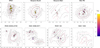 |
Fig. B.1 Maps of HRA regions with NESTs. Grey asterisks represent the YSOs in the area, and coloured markers show the position of NESTs. Symbols indicate whether the significant activity of NESTs is significantly different (triangles for larger, and inverted triangles for lower), or consistent with the average (circles). The colour scale shows the ratio of Class 0/I objects assigned to each NEST. Contours show each region’s relative risk map values, and red contours mark the threshold boundaries f̄C0/I ± σfC0/I separating areas with values different from the average control distribution for each region (solid red contour for the upper limit and dashed for the lower). |
Appendix B.2 IRA regions
EAGLE This HII region in the Serpens constellation, also known as M16, hosts the young cluster NGC 6611 Stoop et al. (2023). We find 23 NESTs that contain 14% of the YSOs in the region. The NEST distribution is dominated by a large group of 19 with average activity, spatially corresponding to NGC 6111 and including a well-populated NEST with NMX = 4.2. Towards the North of the region, we find two active NESTs, with very high values of fC0/I ~ 0.38. West of NGC6111, we find a single, small NEST of average activity but close to the relative risk threshold. There is also a single small, compact NEST of average activity south of the large group, with similar activity to it. This structure is not coincident with those obtained by (K14) or the MST technique (see complementary material). The relative risk pattern is not correlated with the YSO density, as the largest spatial concentration, NGC6111, is of average activity. Areas of large fC0/I ratios are peripheral, notably overlapping with the eastern and Northern NESTs, but displaced from the southern one. The value of Q=0.8 would point to a lack of substructure, but our results indicate that it is a mixed situation, comprising various small-scale significant substructures and a dominant, large-scale concentration.
Rosette The Rosette nebula hosts several young clusters and associations, notably NGC2244. Our analysis finds a rich population of 15 NESTS with significantly different activities and forming various groupings. This is consistent with the low value of Q=0.45, characteristic of substructured distributions. Towards the northwest, we find 3 NESTs less active than average, two of them together and corresponding to the known cluster NGC2244. The rest of the NESTs correlate spatially with groupings reported by Mužić et al. (2022), and also with substructures found by (K14) and the MST. In the centre of the image we find a single NEST of average activity, and all the other NESTs are located in the southeast, forming an elongated arrangement. This large grouping shows a significant activity gradient with NESTs of both high and average activity and broadly overlaps high-density gas structures (Hennemann et al. 2010 and Motte et al. 2010). The relative risk spatial pattern is complex: in the south, it is mostly consistent with the YSO density, and as we move north-east, the relationship degrades and inverts. In the central area, the higher fC0/I values are displaced from the dense NEST and in the north, the high YSO density region is actually of low relative risk.
CepC This region is part of the Cepheus complex, and displays a simple structure consistent with low concentration values (Q = 0.83). We find a single NEST small, compact, and active, with a high value of fC0/I = 22.5%. The relative risk shows a central high fC0/I area and a low-risk NW region, the latter supported by low densities. Our results globally agree with those by Gutermuth et al. (2011), who studied the YSO and dust distribution on the whole complex.
-
NGC2264 This region in Monoceros hosts a rich, well-characterised, YSO population of different evolutionary stages. As one of the regions with the best studied SF history, we have used it as a benchmark to evaluate the methodology in this work, and more detailed results are avaliable as online complementary material.
The complex has two main large substructures: a more evolved northern one around the massive star S-Mon, and a bilobed active cluster Spokes-Cone (see e.g. Nony et al. 2021, and references therein). We find a population of 15 NESTs hosting 15% of the YSOs, consistent with the high level of substructure (Q=0.65) and the general knowledge of the region. NESTs are organised into three groups: a Northern group corresponding to S-Mon with two evolved NESTs, a single evolved NEST towards the west, and a larger group of 12 highly active NESTs in Spokes-Cone. In addition to the general North-South SF gradient of the complex, we detect differences in activity in the Spokes-Cone grouping, with a significant span ∆fC0/I. While all 12 NESTs are active, those in spokes substructure have higher SF than those of the Cone, as reported in Venuti et al. 2018.
Sh2-106 This is an expanding bipolar HII region in the Cygnus X area (Bally et al. 2022). We find three NESTs that account for 19% of all the objects in the region. Two of them are located towards the center of the region, highly active, and seem to trace the same large-scale structure. We detect a separate small NEST in the south with average activity, significantly lower than the central ones. The high value of Q = 0.91 points to the dominance of the central large-scale structure, which also contains a well-populated NEST (NMX = 7.5). The largest values in fC0/I are shifted east from the density peak traced by the largest NEST, but we are cautious due to the very low YSO density values in the peak.
OMC 2-3 This region is part of the Orion Nebula, located between the Orion Nebula Cluster and ONC Flank N, both also part of this work (Peterson & Megeath 2008). The value of Q = 0.7 suggests some degree of substructure, but we only find one very small and compact NEST, active and centered in the field. The global ratio is f̄C0/I = 13.4% close to the HRA boundary. We note that the Orion fields in these samples divide a known large gas filament. The YSO density shows larger values towards the southern boundary, where the very dense main Orion Nebula Cluster is located. The relative risk map has a different distribution from the YSOs, with an elongated high fC0/I area vertically aligned with the filament segment in the field. In addition to density gradients, the division of a region, particularly if it cuts a dense structure, can impact the structural properties of the sample, including key parameters for S2D2 such as the reference comparison density. We performed S2D2 in a sample composed of all 4 regions (here referred to as Orion, OMC 2-3, ONC Flank N, and ONC Flank S), to evaluate these effects. We only retrieved a group of NESTs corresponding to the dominant structure, the Orion Nebula Cluster.
GGD12-15 This is a high mass region, sometimes also identified as IRAS 06084-0611, on the Monoceros R2 complex. We retrieve a group of three small NESTs with 15% of the YSO population and high. The group corresponds to the large central structure in the YSO density, which has Q = 1.0, indicating high concentration levels. The relative risk map is correlated with the YSO density and has a decreasing outward gradient. Our results are consistent with other work. Gutermuth et al. (2011) studied YSOs in the complete Monoceros R2 complex field and in connection with the dust estimates, and our NESTs coincide with their large structure, which overlaps with a peak in the dust. Our results are also compatible with Maaskant et al. (2011), who report a larger concentration of less evolved objects attributed to sequential SF along the line of sight.
SFO 2 This region (also known as IRAS 00013+681,7 BRC2, and S171, Getman et al. 2018b) is part of the Cepheus Loop bubble and close to Be 59, also studied in this work. We find a single NEST, small and compact, tracing the central global concentration (Q = 0.88). The global number of members of this region N = 63 is low, which can produce high relative density ρrel > 30 and large dispersion values. Most of the relative risk map is consistent with the average, with high and low fC0/I values located towards the boundaries, which we note have low densities of YSOs. This young star cluster is located on a bright rimmed cloud, where sequential SF has long been proposed (Sugitani et al. 1995).
RCW36 We analyse the young central cluster in this HII region from the Vela C molecular cloud, characterised by gas expansion patterns (Bonne et al. 2022). We find a single NEST with average activity. The NEST is well populated, with 36 objects corresponding to 12% of the total YSO sample and a relative population value NMX = 7.2. Our results are consistent with a global large-scale concentration, also indicated by Q = 0.9. The relative risk map shows a different pattern from the YSO density: the central concentration is consistent with average, with high (resp low) fC0/I values towards the north (resp south).
Flame Nebula We obtain a group of 9 average NESTs comprising 15% of YSOs in a concentrated distribution (Q=0.96) consistent with he cluster NGC2024. The group is displaced west of the peak in relative risk, and one of the NESTs is close to its significance threshold. The NESTs are roughly coincident with the main filament (Bešlić et al. 2024), but specific comparisons with the gas density need to be performed.
Cep A In this portion of the Cepheus complex, we find a single small and compact NEST, with average activity, and consistent with low levels of spatial concentration (Q = 0.84), similar to Cep C. The relative risk map has a single elongated high-risk peak displaced towards the west from the YSO density peak traced by the NEST, with the eastern part of the field characterised by low fC0/I values.
W40 This region belongs to the Aquila Rift and is close to Serpens South. We find a group of 3 NESTs containing 7% of all YSOs compatible with moderate levels of spatial concentration (Q = 0.85). The large-scale structure traced by NEST is spatially consistent with the highest ranking structure in the hierarchical, large-scale analysis by Sun et al. (2022). The relative risk map shows a very different pattern from the YSO density, with average values in the central area and low values on the West. We only find fC0/I values concentrated on the North and South Eastern corners of the field.
LkHa101 This is an embedded region in the California Molecular Cloud, named by a central Herbig Be star (Wolk et al. 2010 and Getman et al. 2018b). We find three NESTs of average activity, towards the center of the field, consistent with a moderate global large-scale concentration of the YSO sample (Q = 0.84). The central YSO concentration has an average relative risk, with high fC0/I values towards the Southern area where densities are low. Wolk et al. (2010) obtained a catalogue for the region and derived a ratio of ClassIII:ClassII: Classi of 7:5:1, corresponding to a fC0/I ratio of 8%, larger than but consistent with the values f̄C0/I = 6% derived from this sample.
NGC6357 This SF complex in the Sagittarius arm contains 3 known open clusters of similar sizes and estimated ages of ∼ 1 Myr (see e.g. Ordenes-Huanca et al. 2024, and references therein). We obtained 18 NESTs of average activity arranged in three large-scale groupings, compatible with the known substructure of the region and the low values of Q = 0.65. This is one of two IRA regions where all NESTs have lower fC0/I than average, although the difference is not significant. The values of f̄C0/I = 0.06 are on the low side of IRA regions, and the uncertainty σfC0/I is slightly larger, so all possible low values of fC0/I are consistent with the average. The relative risk map shows several high-risk peaks, small and decoupled from the YSO density. Our results are globally consistent with the general knowledge of the complex, host of several bubbles and massive stars.
ONC Flank S: This is another part of the Orion Nebula, with a situation similar to the previously described in OMC2-3. We find a single, small NEST towards the ONC, located North of the observed field. We note that while the number of stars and structural characteristics of this sample are similar to the previous one, the global ratio is very different f̄C0/I = 4%, close to the lower boundary of the IRA regions. The relative risk map is different from the complete YSO distribution, with an East-to-West increasing gradient.
IC348 This region, part of the Perseus complex and close to NGC1333, has a group of 5 NESTs towards the North. IC348 was also analysed in Paper I but using the sample provided by Luhman et al. (2016). The two samples have different spatial coverage and number of stars: the one used in this work has fewer stars and a smaller field. This sample has a northern NEST that was not retrieved by our previous analysis, and, conversely, in Paper I we found a separate NEST towards the South, but the southernmost group of three NESTs and the western one coincide. This is the only IRA region where all retrieved NESTs have significantly low activity. The ratio of Class 0/I objects we obtain, fC0/I = 0.06, is compatible with that of Young et al. (2015), 0.08, but their ratio of Class II objects, 0.73, is much larger than the one in this work fcII = 0.31 . Our estimate of class II members is closer to that of Luhman et al. (2016) ∼ 0.4. The relative risk map shows an increasing N-S gradient. Our global results are consistent with the Perseus analysis in Gutermuth et al. (2011), which shows a Northern concentration of YSOs displaced from the southern peak in dust density.
Appendix B.3 LRA regions
Cep OB 3b This is a well-populated Cepheus region in the late stages of gas dispersal (Karnath et al. 2019), consistently with a low global ratio of Class 0/I objects. We find 8 small NESTs that only account for 6% of the YSOs in the region. NESTs are grouped in three distinct areas, compatible with previously retrieved substructures, and also with the low Q = 0.65 values. Relative risk has a globally complex pattern, with peaks decoupled from the global YSO density. Gutermuth et al. (2011) and Allen et al. (2012) also show a YSO distribution different from that of the gas, with the large eastern and western subclusters only partially overlapping high-density gas. Our results are consistent with residual recent SF associated with gas remnants, and the general knowledge of the region. Additionally, if we use the ratio of objects of Class II fCII as a youth indicator, we find significantly larger values in the western subcluster, in agreement with the fractions of objects with disks found by Allen et al. (2012).
Lagoon Lagoon Nebula, also known as M8, hosts an HII region and open cluster NGC6530. We find 5 average NESTs in the region, organised into two separate groups. The eastern group has 4 NESTs, and the western one is a well-populated NEST with NMX = 6. The different relative weights of both substructures can explain the value of Q = 0.8, indicative of CSR in the box-fractal and radial paradigm. Despite all NESTs being compatible with average, we find significant differences in the activity of both subclusters, ∆fNEST > σfC0/I, with the western subcluster significantly more active than the eastern. Our results are compatible with recent spatiokinematical structures retrieved by Jia et al. (2024). In particular, the western structure would correspond to sub-3, recently formed according to their kinematic tracing analysis, and the eastern clump spatially overlaps with their main substructure, sub-1. Jia et al. (2024) predict that substructure 3 will merge with 1, but the fate of other substructures is unclear, as the picture is very complex. Such a complex scenario agrees with the previous spatiokinematical analysis by Wright & Parker (2019). Their results indicate a strong dynamical evolution of the region, which would have undergone cold collapse from a more extended and substructured distribution.
IC5146 This is a young open cluster in the Cocoon nebula, characterised by an HII region surrounded by filamentary gas structures that are currently forming dense cores (Chung et al. 2024). While this hints to future SF in the region, the current YSO sample we analyse has very low values of fC0/I = 0.03. We find 2 NESTs, tracing the large-scale central concentration (Q = 0.86). Both NESTs are of average activity, and the Southern one is well populated with Nmx = 6.4. The relative risk shows a global decreasing trend from North to South, but we need to remember that fC0/I values are low and the periphery has relatively low YSO density. The Class II relative risk map shows two large-scale structures with significantly high risk. One of them is towards the lower density western structure, and the main one coincides with the YSO concentration, with one NEST showing a significant Class II ratio and the other consistent with average but close to the boundary.
NGC2362 This cluster is characterised by its low extinction and a rich population with several massive stars (Damian et al. 2021). We find 4 NESTs with average recent activity on a sample that shows signs of a strong global concentration (Q = 0.93). Three of the NESTs are grouped towards the centre, while a single one appears on the outskirts towards the North. Regarding the evolutionary stage of the cluster, the classified sample is globally very evolved, with an extremely low ratio of Class 0/I objects (there is only one) and less than 10% of Class II. The relative risk of Class II is mostly consistent with the average, as high/low fCII values are on peripheral, low-density areas.
NGC7160 This open cluster in the Cepheus OB2 region is relatively old (estimates compiled by Mendigutía et al. 2022, indicate an age between 8 and 15 Myr), and we accordingly find a very low fC0/I = 0.01 (with only one source), and also a very low ratio of Class II objects fCII = 0.05. We note that while the region has a low global number of members N = 96, almost all of them are classified as stellar. We retrieve two small NESTs of average activity located towards the center of the region tracing the large-scale overdensity (Q = 0.9). The Class II relative risk map shows a descending patterns towards the East, with larger values on the south.
Be 59 Berkeley 59 is the main cluster within an HII region of Cepheus OB4, close to SFO2. We find 5 NESTs of average activity in a large group consistent with a large-scale concentration, also indicated by Q = 0.86. The central part of the relative risk map is consistent with average with high areas towards the west and on the easter boundaries. The distribution of Class II sources is more complex, with several areas of both high and low activity surrounding the central area which is consistent with average. These results are broadly consistent with the triggered SF scenario explored by Mintz et al. (2021), with the whole Cep OB4 complex having a low ratio of Class I/II objects in the cluster and increasing towards the outskirts of the extended structure.
Carina As previously mentioned, this region was already analysed in Paper I where we used a physical 1000AU merging limit, while here the physical distance associated with the constant 2 resolution limit corresponds to 4.6 kAU. The results are very similar, with 10% of the members grouped in 19 NESTs that trace most of the known open clusters in the region. Trumpler 14 is still the dominant structure in the sample, traced by a group of NESTs that includes the most populated one (NMX = 25.60). There were only 2 members of the region classified as Class 0/I, meaning extremely low values of fC0/I = 0.001, so all NESTs (and actually most of the region) have fC0/I values consistent with average. The value fCII = 0.1 is also relatively low, and the Class II relative risk map has peaks all over the region, although none coincide with the position of NESTs. While the general picture of the region from this sample points to very low recent SF activity, other studies show relevant age spans in Carina and very young age estimates for Trumpler 14 (see e.g. Itrich et al. 2024, and references therein), which could point to some recent SF in the region undetected in this study.
ONC Flank N: This field is a peripheral part of the Orion Molecular Cloud where we did not retrieve any significant small-scale substructure. The distribution generally agrees with CSR, as pointed by Q = 0.78 and the high values of ρrel. This region corresponds to the peripheral part of the Orion molecular cloud filament, so the previously mentioned caveats regarding the window selection hold. The fC0/I map shows two high-risk areas, but we must note that they are only traced by the few Class 0/I members of the region. The class II relative risk map, with a large support, shows significantly high values on the southern boundary, towards the large gas filament.
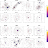 |
Fig. B.2 Maps of IRA regions, with the same symbols as in Figure B.1 |
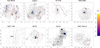 |
Fig. B.3 Maps of LRA regions with NESTs, with the same symbols as in Figure B.1 |
Appendix B.4 Flagged regions
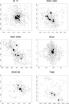 |
Fig. B.4 Maps of regions with a classified subsample flagged as non representative. Grey dots represent the YSOs in the area, and black markers show the position of the centroids of NESTs. |
Most of these regions are very embedded, high-mass regions, where the presence of gas and massive stars hinders observations. Indeed, a substantial fraction of members in these samples do not have the required IR photometric information at all, or with insufficient quality for classification (G09).
Orion Main cluster in the Orion cloud, very well studied as one of the closest examples of active high mass SF. Peripheral sections of this same cloud have been previously analysed as part of this work (namely ONC Flank N, ONC Flank S, and OMC 2-3). The cluster is highly embedded, and 55% of the objects in our sample remained unclassified due to poor photometry. We retrieve a group of 13 NESTs on the centre, tracing a single large-scale concentration. The structural simplicity of this region is supported by the value Q = 0.87 and the presence of well-populated NESTs (NMX = 5.80). Some authors have long observed age / evolutionary outward gradient from the filament (e.g. Getman et al. 2018a; Stutz & Gould 2016). Despite the attention received by this region, there are still open questions, including debate on global formation scenarios and whether SF was continuous or episodic (e.g. Alzate et al. 2023; Kounkel et al. 2022, and Beccari et al. 2017).
M17 This is a very dynamic and active region, host of a large population of massive stars and the very young, well-populated, open cluster NGC 6618. Due to the associated observational difficulties, 86% of the members in this sample could not be classified due to the lack of photometry of enough quality. We find a group of 19 NESTS containing 18% of the YSO sample that traces a high-density large-scale YSO concentration (Q = 1.01). The history of the cluster is still under discussion, particularly the role of a nearby OB group as the initial trigger of SF in the area (see Stoop et al. 2024, and references therein).
RCW38 RCW 38 is known as one of the closest high-mass star-forming regions. In this YSO sample, we could not classify 59% of the members due to photometric quality issues. We retrieve a total of 6 NESTs, 5 of which trace the single, large-scale central YSO overdensity, supported by Q = 0.91 and NMX = 26.75. We also find a separate single, small and compact NEST towards the North. Fukui et al. (2016) proposed cloud-cloud collision as the trigger of the formation of massive stars in the region.
NGC1893 NGC 1893 is a young open cluster embedded in an HII region (Damian et al. 2021). Despite its moderate extinction, it is the most distant, d = 3.6 Kpc and 44% of its members did not have sufficient photometric information for classification. It is the only region with a relevant fraction of objects classified as non-stellar, 11%. There is clear large-scale overdensity in the region, also supported by Q = 0.92, and our results suggest some level of substructure within it. We retrieved 14 NESTs that contain 12% of the members of the region. 12 NESTs are visually aligned with a large-scale elongated density structure, while the other two form a distinct group towards the north.
Trifid: Trifid is a bright HII nebula in Sagittarius, also known as M20, host of open cluster NGC6514. 53% of the sample did not meet quality requirements. We find three small NESTs containing 9% of the YSOs, consistent with a substructured distribution (also suggested by Q = 0.69). The two central NESTs correspond to the main cluster, and the southern NEST is located on a filament cut by the field boundary (as indicated in K14). In this region, cloud-cloud collision has also been proposed as star formation mechanism (Torii et al. 2017), although recent kinematical studies of YSOs propose that expansion of an HII region (Kuhn et al. 2022) could have triggered star formation.
NGC6334 This is a high-mass complex that contains HII regions and high-density ridge, where 60% of the sources lacked the required photometric information. The region is highly active and contains a considerable population of dense cores with complex spatial distribution and various evolutionary stages which was attributed to hierarchical fragmentation by Sadaghiani et al. (2020). We find 7 small, compact NESTs that only contain 6% of all the YSOs dispersed over a large portion the region, which has a value of Q = 0.71, pointing to a highly substructured distribution. The positions of NESTs seems close to the hubs and ridges identified in the molecular cloud (studied in Russeil et al. 2013 and Tigé et al. 2017). At this stage, the evidence is consistent with most hierarchical SF scenarios, and further analyses considering the molecular cloud and overlaps between NESTs and the cloud structures would be interesting.
All Tables
Summary statistics of the classification results in the region sample with accepted classifications.
Classification of NESTs according to their evolutionary stage estimated from fC0/I, grouped by the recent activity regime of the host region.
All Figures
|
Fig. 1 Spatial distribution and relative-risk maps for NGC2264. Left: spatial distribution of objects in NGC2264. Dots represent each source in the complete sample, coloured according to the evolutionary stage classification described in Section 2.3.1 (green for Class 0/I, red for Class II, black for Class III, and empty for unclassified and non-stellar objects). Right: four-panel composite showcasing the associated densities and relative-risk maps. Top left: KDE estimate corresponding to the classified sub-sample in the left panel. Top right: relative-risk maps of Class 0/I objects. Bottom panels: relative-risk maps of Class II and Class III objects. |
| In the text | |
|
Fig. 2 Relative density of NESTs compared to that of the region’s ρrel versus Q structural parameter. The marginal distributions are shown as density profiles on their respective axes. The hatched zones indicate values of Q corresponding unequivocally to sub-structured (Q ⪅ 0.7) and concentrated (Q ⪆ 0.87) distributions. |
| In the text | |
|
Fig. 3 Stacked bar diagram representing the fraction of stellar objects of each evolutionary state in each (not flagged) region, ordered by Class 0/I fraction. The colour of the bars represents the regime attributed to each region: purple for HRA regions, green for IRA regions, and yellow for LRA regions, as explained in the main text. The intensity of each bar represents the different classes of objects in each region, with darker shades representing less evolved objects. |
| In the text | |
|
Fig. 4 Bar plots display the average fraction of C0/I objects in each region, with dotted black lines indicating the limits for categorizing NESTs as high-activity or low activity, that is |
| In the text | |
|
Fig. 5 Comparison of structures from K14 and G18. Top left: histogram of the size of NESTs (red) and the structures from K14 and G18 in kilo astronomical units. Top Right: histogram of relative average density and the structures from K14 and G18. Bottom: grey bars show the average ratio, f̄C0/I, in each region, with small horizontal dotted lines showing the limits f̄C0/I ± σfC0/I. Red (resp. black) dots show the median values of fC0/I from the relative-risk maps in the area occupied by the convex hull of NESTs (resp. structures from K14 and G18), with error bars representing the first and third quartiles. Solid red (resp. black) lines join the median values of fC0/I for NESTs (resp. K14 and G18) to help compare the values. Finally, vertical lines separate the HRA, IRA, and LRA regimes. |
| In the text | |
|
Fig. 6 Maps of selected HRA regions with NESTs. Grey dots represent the YSOs in the area, and coloured markers show the position of NESTs. Symbols indicate whether the activity of NESTs is significantly different (triangles for larger and inverted triangles for lower activity) or consistent with the average (circles). The colour-scale shows the ratio of Class 0/I objects assigned to each NEST. Contours show each region’s relative-risk map values, and red contours mark the threshold boundaries, f̄C0/I ± σfC0/I, separating areas with values different from the average control distribution for each region (solid red contour for the upper limit and dashed red contour for the lower limit). |
| In the text | |
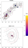 |
Fig. 7 Maps of selected IRA regions with NESTs, with the same symbols as in Figure 6. |
| In the text | |
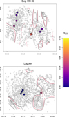 |
Fig. 8 Maps of selected LRA regions with NESTs, with the same symbols as in Figure 6. |
| In the text | |
|
Fig. B.1 Maps of HRA regions with NESTs. Grey asterisks represent the YSOs in the area, and coloured markers show the position of NESTs. Symbols indicate whether the significant activity of NESTs is significantly different (triangles for larger, and inverted triangles for lower), or consistent with the average (circles). The colour scale shows the ratio of Class 0/I objects assigned to each NEST. Contours show each region’s relative risk map values, and red contours mark the threshold boundaries f̄C0/I ± σfC0/I separating areas with values different from the average control distribution for each region (solid red contour for the upper limit and dashed for the lower). |
| In the text | |
|
Fig. B.2 Maps of IRA regions, with the same symbols as in Figure B.1 |
| In the text | |
|
Fig. B.3 Maps of LRA regions with NESTs, with the same symbols as in Figure B.1 |
| In the text | |
|
Fig. B.4 Maps of regions with a classified subsample flagged as non representative. Grey dots represent the YSOs in the area, and black markers show the position of the centroids of NESTs. |
| In the text | |
Current usage metrics show cumulative count of Article Views (full-text article views including HTML views, PDF and ePub downloads, according to the available data) and Abstracts Views on Vision4Press platform.
Data correspond to usage on the plateform after 2015. The current usage metrics is available 48-96 hours after online publication and is updated daily on week days.
Initial download of the metrics may take a while.