| Issue |
A&A
Volume 697, May 2025
|
|
|---|---|---|
| Article Number | A118 | |
| Number of page(s) | 14 | |
| Section | Galactic structure, stellar clusters and populations | |
| DOI | https://doi.org/10.1051/0004-6361/202450890 | |
| Published online | 21 May 2025 | |
Binary-single interactions with different mass ratios
Implications for gravitational waves from globular clusters
1
Institut de Ciències del Cosmos (ICCUB), Universitat de Barcelona (IEEC-UB),
Martí Franquès 1,
08028
Barcelona,
Spain
2
Leiden Observatory, University of Leiden,
Niels Bohrweg 2,
2333
CA Leiden,
The Netherlands
3
ICREA,
Pg. Lluís Companys 23,
08010
Barcelona,
Spain
4
Gravity Exploration Institute, School of Physics and Astronomy, Cardiff University,
CF24 3AA,
UK
★ Corresponding author: bruno.randof@gmail.com
Received:
28
May
2024
Accepted:
23
March
2025
Context. Dynamical interactions in star clusters are an efficient mechanism to produce the coalescing binary black holes (BBHs) that have been detected with gravitational waves (GWs).
Aims. We want to understand how BBH coalescence can occur during – or after – binary-single interactions with different mass ratios.
Methods. We perform gravitational scattering experiments of binary-single interactions using different mass ratios of the binary components (q2 ≡ m2/m1 ≤ 1) and the incoming single (q3 ≡ m3/m1). We extract cross-sections and rates for (i) GW capture during resonant interactions; (ii) GW inspiral in between resonant interactions and apply the results to different globular cluster conditions.
Results. We find that GW capture during resonant interactions is most efficient if q2 ≃ q3 and that the mass-ratio distribution of BBH coalescence due to inspirals is ∝ m1−1q2.9﹢α, where α is the exponent of the BH mass function. The total rate of GW captures and inspirals depends mostly on m1 and is relatively insensitive to q2 and q3. We show that eccentricity increase in direct (that is, non-resonant) encounters approximately doubles the rate of BBH inspirals in between resonant encounters. For a given GC mass and radius, the BBH merger rate in metal-rich GCs is approximately double that of metal-poor GCs, because of their (on average) lower BH masses (m1) and steeper BH mass function, yielding binaries with lower q.
Conclusions. Our results enable the mass-ratio distribution of dynamically formed BBH mergers to be translated to the underlying BH mass function. The additional mechanism that leads to a doubling of the inspirals provides an explanation for the reported high fraction of in-cluster inspirals in N-body models of clusters.
Key words: black hole physics / gravitational waves / stars: kinematics and dynamics / globular clusters: general
© The Authors 2025
 Open Access article, published by EDP Sciences, under the terms of the Creative Commons Attribution License (https://creativecommons.org/licenses/by/4.0), which permits unrestricted use, distribution, and reproduction in any medium, provided the original work is properly cited.
This article is published in open access under the Subscribe to Open model. Subscribe to A&A to support open access publication.
1 Introduction
The first binary black hole (BBH) coalescence was detected in 2015 by LIGO (the Laser Interferometer Gravitational Wave Observatory) (Abbott et al. 2016). In the first three observing runs of the LIGO-Virgo-Kagra (LVK) Collaboration, a total of 90 compact binary coalescences (CBCs) were reported, involving black holes (BHs) and neutron stars (NSs) (Abbott et al. 2021). At the time of writing, around 80 more were found in O4a. Gravitational wave (GW) astronomy allows us to observe the Universe from a completely new perspective, unveiling phenomena that remain invisible to the traditional electromagnetic observations. The dominance of BHs involved CBCs has raised the question of how these binaries form and eventually inspiral. The literature on this topic is rich and multiple formation scenarios have been proposed for CBC. We refer to the review by Mandel & Broekgaarden (2022) and references therein for an overview. Important for this work is that – especially for massive BBHs – dynamical assembly has been suggested to be an efficient mechanism for creating GW sources (e.g. Portegies Zwart & McMillan 2000; Rodriguez et al. 2015; Banerjee 2018; Di Carlo et al. 2019).
In this paper, we are concerned with the dynamical interactions of BHs that lead to mergers within the cores of globular clusters (GCs). In GCs, there is a large number of stellar remnants such as BHs and NSs, which are formed during the early stages of the cluster, when the massive stars end their lives. Those compact remnants sink towards the centre of the cluster due to dynamical friction. It is in this environment where interactions are frequent, and the formation of BBHs is driven by the energy need for the relaxation of the GC (Hénon 1975; Breen & Heggie 2013). Tight binaries harden as the result of interactions (Heggie 1975), and give away part of their energy to their surroundings in the form of kinetic energy. After many encounters, the BBHs can be compact enough to merge through the emission of GWs. It is believed that these binary systems could be responsible for a significant fraction of the massive mergers identified by the LVK collaboration to date (e.g. Rodriguez et al. 2016; Antonini et al. 2023). The interactions that drive the hardening process of the BBH can be binary-single encounters, or higher order configurations such as binary-binary encounters (Zevin et al. 2019).
The topic of this study is the eventual coalescences of BBHs in GCs through binary-single encounters. Particularly, we conduct scattering experiments as in Hut & Bahcall (1983), but with unequal component masses. Because BHs of different masses coexist and interact in GCs, the inclusion of different masses in our simulations allows us to better understand the phenomena surrounding these BH interactions. For example, including arbitrary masses can shed light on the mass-ratio distribution from mergers detected by the LVK collaboration. To better represent binary-single encounters in GCs, we weigh our scattering events according to the mass distributions of the three bodies, which are obtained from a model for BBH coalescences in GCs (as in Antonini & Gieles 2020b). Although useful, the unequal-mass regime further complicates the already complex equal-mass three-body problem. It is for this reason that we use Newtonian dynamics: this allows us to determine the dynamics of the system not by the absolute masses, but rather by the mass ratios of the BHs, reducing the dimension of the parameter space by one and simplifying the analysis. The elephant in the room is that we aim at understanding the physics surrounding BH mergers with Newtonian dynamics, which at first glance appears to be contradictory. The work of Samsing et al. (2014); Samsing (2018); Samsing et al. (2020), Antonini & Gieles (2020b) shows that the rate of inspiral in post-Newtonian scattering experiments can be well described by simple Newtonian theory using a minimum distance/eccentricity criterion for inspiral to occurs. We can, therefore, determine a posteriori which of the Newtonian interactions would lead to mergers.
In parallel to the GW implications of binary-single encounters, we also use our unequal-mass simulations to revisit some generalities of the three-body problem. Extensive work has been done in the equal-mass case (Hut & Bahcall 1983; Heggie & Hut 1993), as well as in the unequal-mass case (Hills & Fullerton 1980; Spitzer 1987; Sigurdsson & Phinney 1993; Heggie et al. 1996; Quinlan 1996). The main work has been put into the different outcomes that can result from a binary-single encounter, such as exchanges of one of the components, close approaches, and eccentricity or energy changes in the initial binary. With the growing interest in GWs, later literature on binary-single interactions also includes the possibility for CBCs (Gültekin et al. 2006; Samsing et al. 2014; Ginat & Perets 2023). We build upon their work by exploring some yet unknown intricacies of resonant interactions. As we will explain later on, during a resonant binary-single interaction, a bound but unstable three-body system is formed, where the three components approach each other repeatedly. After such an encounter, the remaining binary usually has an increased binding energy, and its eccentricity can be completely different from its initial value. We study how this energy change, the final eccentricity distribution, and the number of repeated approaches depend on the masses of the triplet.
This paper is organised as follows: in Section 2 the terminology and settings of the binary-single scattering problem are explained. We also describe the initial conditions required to fully determine a scattering experiment, followed by a description of the software package used to run the simulations. In Section 3 we present general results of the binary-single scattering experiments. In Section 4 we apply the results of the scattering experiments to different GC conditions. In Section 5 we focus our analysis to the specific case of BBH coalescences happening in GCs. The limitations of our analysis are discussed in Section 6, and our findings are summarised in Section 7.
2 Methods: Scattering experiments
2.1 The binary-single scattering problem
Binary-single scattering refers to the specific scenario where a binary interacts gravitationally with a single body. This work seeks to understand the dynamics, outcomes, and effects of these interactions, with a particular focus on encounters involving BHs of different masses. The simulations are done in the Newtonian point-mass limit. It is for this reason that in this Section and in Section 3, the point masses will be referred to as bodies. From now on, the components of the initial binary are labelled as 1 and 2, with 1 being the heaviest, and the single body is labelled as 3.
The terminology used in the gravitational scattering problem has some analogies with particle physics experiments. When the final three-body system has no bound states between bodies, we say that the system is ionised. Furthermore, when the final binary is composed of two different bodies than the initial binary, we refer to the outcome as an exchange, while a preservation refers to a final binary with the same components as the initial binary. More analogies with particle physics are found in Appendix A, where we discuss the use of cross-sections.
The gravitational three-body problem is in almost all cases chaotic, and some of the scatterings can allow for temporarily bound three-body systems: we call these interactions resonant. A way to clearly define whether an interaction is resonant is through the number of minima in s2 as a function of time, defined as
 (1)
where rij is the distance between bodies i and j. For very early and very late times, s2 is arbitrarily large, because at least one of the three bodies is at infinite distance from the binary. During the closest interaction, s2 can have either one or multiple minima: this number of minima is called the number of intermediate states NIMS. If the interaction is such that NIMS > 1, we label it as resonant. Otherwise, if s2 has a single minimum (NIMS = 1) the interaction is non-resonant, or direct (Heggie et al. 1996). We consider two consecutive minima to be distinct if the value of s2 at the maximum is at least twice that of the minima (following McMillan & Hut 1996).
(1)
where rij is the distance between bodies i and j. For very early and very late times, s2 is arbitrarily large, because at least one of the three bodies is at infinite distance from the binary. During the closest interaction, s2 can have either one or multiple minima: this number of minima is called the number of intermediate states NIMS. If the interaction is such that NIMS > 1, we label it as resonant. Otherwise, if s2 has a single minimum (NIMS = 1) the interaction is non-resonant, or direct (Heggie et al. 1996). We consider two consecutive minima to be distinct if the value of s2 at the maximum is at least twice that of the minima (following McMillan & Hut 1996).
Among resonant interactions, we distinguish democratic resonances from hierarchical resonances (Heggie & Hut 1993). Democratic resonances are those that do not favour the interactions of a single pair of bodies with respect to the other two pairs, while hierarchical resonances are characterised by having a pair of bodies strongly interacting, with the third body on a wider orbit around them. Even though sometimes it is easily seen which kind of resonance corresponds to a given interaction, there is no exact line that separates democratic and hierarchical interactions. For example, in nature some resonant interactions will live enough to oscillate from democratic to hierarchical (and vice versa), making the classification problematic. It is for this reason that we are not separating on this classification, but it is worth mentioning, to illustrate the richness and depth of the gravitational scattering problem.
Moreover, one may also consider the formation of stable three-body systems. If systems like the Sun-Earth-Moon exist, then why are we not considering them as possible outcomes of a scattering? The answer to this question is that scattering events are unable to form stable and bound three-body systems, because the set of initial conditions that lead to a stable three-body system is of measure zero with respect to the initial hyperparameter space. A rigorous proof can be found in Chazy (1929), but Hut & Bahcall (1983) give an intuition for this unlikeliness. A stable three-body system that formed from a binary-single scattering event should be stable for the infinite future. But, if we consider Newton’s time reversibility, we expect the system to be stable for the infinite past, which contradicts the assumption of the system being created by a scattering event.
Our methods to identify GW captures and inspirals in our Newtonian simulations are defined in Section 5.1 and Section 5.2, respectively. For extended bodies, an additional possible outcome is a direct collision (for stellar collisions, see e.g. Fregeau et al. 2004). The cross-section (defined in Appendix A) for a collision between NSs is orders of magnitude lower than that of the other types of mergers (Samsing et al. 2014), and because we only consider BHs, we do not consider collisions in this work.
Parameters needed to specify the initial conditions of a scattering simulation, including their corresponding ranges and the distributions.
2.2 Description of the code and units
To simulate the binary-single scattering events, we use the STARLA B software package. STARLAB is a collection of tools designed to simulate and analyse the dynamical evolution of star clusters, which is described in McMillan & Hut (1996). Within STARLA B, the module SCATTER3 simulates binary-single scattering events using Newtonian physics. It uses a fourth-order variable time step Hermite integrator (described in Makino & Aarseth 1992). To keep integration errors under control, SCAT-TER3 uses a technique developed in Hut et al. (1995) that ensures the symmetry in time, which guarantees that the energy and momentum are kept constant in periodic orbits.
Part of the complexity of the three-body problem is the amount of parameters that need to be specified in order to fully determine the initial conditions. In the point-mass limit, each body requires information of its position, velocity and mass, a total of seven parameters. Therefore, three bodies require 21 parameters. Thankfully, the symmetries of the system allow for a considerable reduction in the number of parameters. In addition, the scale invariance in the physical dimensions of length, time and mass allow for a further reduction of parameters.
We adopt units in which the semi-major axis (SMA) a of the initial binary, the gravitational constant G, and the mass of the initial binary m12 are G = a = m12 = 1. The initial conditions required to simulate a binary-single scattering can be reduced to nine parameters, given in Table 1 (Hut & Bahcall 1983). The impact parameter is given in units of a, and the velocity v is the relative velocity between the binary and the field BH at infinity. We define  as the velocity in units of the critical velocity vc, defined as the relative velocity that makes the energy of the three-body system to be zero:
 (2)
with m123 ≡ m12 + m3. Note that if
(2)
with m123 ≡ m12 + m3. Note that if  , the energy of the three-body system is negative, which implies that ionisation is physically impossible. If
  , the energy of the system is positive. Therefore, bound three-body systems are not permitted, and resonant interactions do not happen.
For this work, we define the mass ratios q2 ≡ m2/m1 and q3 ≡ m3/m1. We explore different values of q2 and q3 in the range [0.1, 1], spaced in steps of 0.05. For each combination of q2 and q3, 31 250 encounters were simulated (for a total of  encounters). This order of magnitude was selected to make the statistical error of mergers in each bin sufficiently low. Following Table 1, the encounters were simulated with eccentricities sampled from a thermal distribution pe(e) = 2e (Jeans 1919), randomly sampled angles, a velocity v = 0.1 , and impact parameters equispaced in b2 in the range b ∈ [0, bmax]. The maximum impact parameter bmax is chosen heuristically by imposing the condition that no resonant encounters happen for b ≳ 0.6bmax. Fewer than 0.1% of the encounters were discarded, either because they were unresolved or because NIMS > 5001.
3 Results: Generalities of unequal-mass encounters
In this section we present results obtained from our binary-single scattering events with unequal-masses. These results are not restricted to BHs, but are general for all binary-single scatterings. The focus is on understanding how the behaviour of resonant interactions varies with the masses of the different bodies.
3.1 Binding energy change for arbitrary masses
Here we obtain the mean change in the binding energy of the binary after a resonant interaction. First, we define  as the absolute value of the binary binding energy
 (3)
(3)
This binding energy can increase or decrease through interactions with a third body. The relative change in  is Δ, defined as
 (4)
(4)
Note that Δ goes from -1, corresponding to binary ionisation, to ∞, implying the collapse of the binary.
From here on we will focus on Δr, which defines the energy change only due to resonant interactions (see Appendix A). It is generally assumed that during a binary-single resonant encounter, the binary increases its binding energy by around a 20% (Spitzer 1987; Heggie & Hut 1993; Quinlan 1996; Portegies Zwart et al. 2010). Nonetheless, the validity of this result is restricted to the equal-mass case. In Fig. 1 we show how ⟨Δr⟩ behaves as a function of m3/m12, where we have realised the fit
![$\langle \Delta_{\rm r}\rangle \simeq \Delta_0\left[1- {\rm exp}\left(-A\frac{m_3}{m_{12}}\right)\right] ,$](/articles/aa/full_html/2025/05/aa50890-24/aa50890-24-eq12.png) (5)
(5)
with Δ0 ≡ ⟨Δr⟩ (m1 = m2 = m3) = 0.2 and A = 7.0. This fit is restricted to m3 ≤ m12. From now on, Equation (5) is used for all calculations that require ΔΓ. We stress that the value of ⟨Δr⟩ is independent of the cross-section, and well-behaved when bmax → ∞. We choose as x-axis the ratio m3/m12 rather than q3, because for the latter the data is noisier at low values of q3.
Although our results agree qualitatively with what Hills & Fullerton (1980) found, our values of ⟨Δr⟩ are a factor of ~2 higher for m3/m12 ≲ 0.1 and a factor of ~4 lower for m3/m12 ~ 1. We note that their encounters were head-on, and we can reproduce their results with our runs with b = 0. These head-on events are unrealistic, and they are physically different from more realistic scatterings with b ≠ 0 due to the difference in angular momentum and in ⟨Δr⟩.
A dynamically assembled BBH in a GC tends to contain the two most massive BHs in the cluster. The eventual binary-single encounters happen with the binary’s stellar surroundings, where bodies generally have masses below m12. In the case of interactions with stars, the difference in mass can even reach two orders of magnitude. In this scenario, Equation (5) implies that ⟨Δr⟩ is generally lower than 0.2. For the BH mass functions assumed in Section 4 we find typical values of Δr ≃ 0.15–0.17, not very different from the equal-mass value of 0.2.
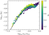 |
Fig. 1 ⟨Δr⟩, in units of Δ0, as a function of m3/m12. Each data point represents a different combination of q2 and q3. The solid line is the fitted function. |
3.2 Number of intermediate states
The number of intermediate states in a resonant encounter, NIMS, is crucial, as the GW capture probability depends linearly on it (see Section 5). For equal masses, ⟨NIMS⟩ ≃ 20 (Samsing 2018), but its behaviour for unequal masses is unknown.
In Fig. 2 we show how ⟨NIMS⟩ behaves in the unequal-mass case. This quantity is maximised in the region where m2 ≃ m3, which also includes the equal-mass case. In this region, ⟨NIMS⟩ ≃ 20, but outside of it ⟨NIMS⟩ drops considerably.
We can intuitively understand this as follows: if one of the bodies is less massive than the other two, then that body is most likely to be ejected (Heggie 1975; Sigurdsson & Phinney 1993; Heggie et al. 1996). The probability of ejection per intermediate state is high and fewer IMSs are, therefore, needed to end a resonant interaction. Meanwhile, if m3 ≃ m2, the probability of ejection per IMS is lower because there is no obvious candidate for ejection and more IMSs are required to end the interaction. The highest number is for equal masses, when the interaction is democratic.
We now present a more rigorous explanation for the behaviour of NIMS. In this derivation, we followed the derivation found in Samsing (2018) and Fabj & Samsing (2024), but generalising it to arbitrary masses (some steps are explained more in detail in the referenced papers). Let us begin by decomposing the triplet during one IMS into a temporary binary of SMA aIMS and (positive) binding energy  , and a single body that orbits the binary on a wider orbit. We assume that, during each IMS, the energy of the binary is randomly sampled from a distribution
 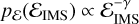 , where we specify the value of γ later on. In the hard binary limit, if
  is higher than the energy of the initial binary
  , then the remaining energy necessarily goes to the single, and the interaction ends with an ejection. In the other hand, if
  , the binary absorbs part of the single’s energy and it remains bound until the next IMS. Then, NIMS can be approximated by (Samsing 2018)
 (6)
(6)
where amax is the maximum value that aIMS can have, or equivalently, the SMA at which EIMS is minimised. Consider the case q3 < q2, and we assume that the temporary binary is always composed by the two heaviest bodies in the triplet (in this particular case, bodies 1 and 2).  attains its minimal value when the system is not decomposed into a binary and a single any more, but by three bodies orbiting each other at the same SMA amax. From energy conservation, this condition is fulfilled when
 (7)
(7)
In combination with ,Equation (6), we obtain
 (8)
(8)
Because of symmetry we have
 (9)
(9)
because after the first intermediate state there is no memory of the initial conditions and the same arguments apply. As for the exponent γ, in Stone & Leigh (2019) it is set at a value between 3.5 and 4, depending on the angular momentum of the system, while Heggie (1975) finds 4.52.
The predictions from Equation (9) are displayed in Fig. 3, where we choose γ = 3.75, so that ⟨NIMS⟩ ≃ 20 in the equalmass regime. We can see that, even though Equation (9) does not predict exactly the behaviour observed in the simulations, it can explain qualitatively why ⟨NIMS⟩ peaks if q2 = q3, and also it can explain the weaker dependence on q2 × q3 . As it can be seen, the theoretical peak is narrower than the experimental one. This difference between theory and experiment can stem from the assumption that the temporary binary always contains the twomostmassivebodies. Itmay be the case that the peak widens by relaxing this condition, and allowing the temporary binary to sometimes contain the lightest body. The distribution would also be broader for smaller values of γ.
3.3 Eccentricity distribution
It is often assumed that the eccentricity of the binary that remains after a resonant encounter follows a thermal distribution pe (e) = 2e. Stone & Leigh (2019) show that for high angular momentum binary-single interactions3 the resulting eccentricity distribution is mildly super-thermal: pe (e) = (6/5)e (1 + e). In Fig. 4 we compare the eccentricity distribution in the equal and unequal-mass regimes with both the thermal and the mildly superthermal distributions. The eccentricity in the equal-mass case agrees with the mildly superthermal distribution, which agrees with the result of Stone & Leigh (2019). Meanwhile, in the unequal-mass regime, the data agrees with a thermal distribution. According to Ginat & Perets (2023), an equalmass binary interacting with a lower mass body is theoretically expected to have a highly superthermal distribution. This discrepancy is explained by the lower limit in the angular momentum of the system. While in the referenced paper the lower limit is zero, a lower limit close to the one found in our scatterings can reproduce the results from Fig. 4 (Ginat, private communication).
Note that in the unequal-mass case, although the eccentricity agrees with a thermal distribution, there is a peak at e ≃ 1. This peak is an artefact from our simulations that appears in encounters with q3 ≃ 1, q2 ≃ 0.1 and zero impact parameter. For these encounters, the secondary component of the binary is so light that it barely perturbs the other two bodies. Therefore, the secondary mass orbits a principal mass that is nearly sitting still. In the other hand, the single body, as massive as the primary mass and with zero impact parameter, follows a head- on collision towards the binary’s centre of mass, almost where the primary mass rests. In this regime, the eventual interactions are extremely eccentric. This artifact appears because of the way that b is sampled: we simulate a lot more encounters with impact parameter being exactly zero than in nature, where the probability of a head-on encounter is zero. If we exclude the set of interactions with b = 0, this artifact disappears.
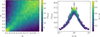 |
Fig. 2 Left: ⟨NIMS⟩ for resonant encounters with different mass ratios. Right: ⟨NIMS⟩ for resonant encounters, as a function of q3/q2. The error bars correspond to V2 times the standard error of the mean. |
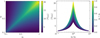 |
Fig. 3 Left: theoretical ⟨NIMS⟩ for resonant encounters with different mass ratios. Right: theoretical ⟨NIMS⟩ for resonant encounters, as a function of q3/q2. |
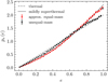 |
Fig. 4 Eccentricity distribution after a democratic resonance. For the approximate equal mass case, the data points were selected by imposing the condition q2, q3 ∈ [0.5,1]. For the unequal-mass case, the data points were selected by imposing the condition q2 ∈ [0.1,0.4] or q3 ∈ [0.1,0.4]. The dashed lines represent the thermal distribution, and the solid line represents the mildly superthermal distribution. |
4 Binary-single BH interactions in globular clusters
In this Section, we describe a simple model for a globular cluster, which includes the properties of its BH population and its central BBH. Our model follows closely the model of Antonini & Gieles (2020b).
4.1 Globular cluster properties
We start by considering the total energy of the cluster, which is given by  , with Mcl the cluster mass and rh the half-mass radius. In steady post-collapse evolution, the rate of change of Ecl (excluding the negative energy locked in binaries) is (Hénon 1961; Gieles et al. 2011; Breen & Heggie 2013)
 (10)
(10)
with ζ ≃ 0.1 (Hénon 1961; Alexander & Gieles 2012; Gieles et al. 2011), and trh the half-mass relaxation time, given by (Spitzer & Hart 1971)
 (11)
(11)
Here, ⟨mall⟩ ≃ 0.5 M⊙, ln Λ ≃ 10, is the Coulomb logarithm which we assume to be constant, and ψ = 1 for equalmass clusters. The one-dimensional velocity dispersion of the cluster is
 (12)
(12)
For a King (1966) model with W0 = 7, the central escape velocity is given by (Antonini & Gieles 2020b)
 (13)
(13)
4.2 Properties of the BH and BBH populations
We assume the presence of a single BBH at the core of the cluster, which contains the heaviest BH within the GC, with mass m1 = mmax, and the second heaviest BH, with mass m2 ∈ [5M⊙, m1]. In this range, we assume a power-law mass function with slope α and adopt two values for α and mmax to mimic metal-poor and metal-rich progenitor stars. We use the rapid single-star evolution (SSE) code (Hurley et al. 2000) with recent updates for massive star winds and BH masses by Banerjee et al. (2020) to determine BH mass functions for 0.01 solar (Z = 1.4 × 10⁻⁴; [Fe/H] = −2) and solar metallicity (Z = 0.014; [Fe/H] = 0). We find mmax ≃ 25 M⊙ for metal-rich clusters, and mmax ≃ 50 M⊙ for metal-poor clusters. Following Heggie (1975); Antonini et al. (2023), the BBH has a mass ratio q2 that follows a distribution  , with α2 = 3.5 + α. Here, α = −0.5 for metal-poor clusters, and α = ࢤ2.3 for metalrich clusters. At the core, we assume a density of field BHs
  , where the additional +1 in the index (i.e. flatter) is because of mass segregation (Portegies Zwart et al. 2007)4. The field BHs that interact with the binary have a mass m3 ∈ [5mΘ, m1] that follows a distribution
  , with α3 = 3/2 + α. The additional flattening of +1/2 with respect to the central BH mass function is because of the assumption of equipartition, which (in the gravitational focusing limit) increases the interaction rate with more massive BHs because of their lower velocities (Antonini & Gieles 2020b). In principle, it is possible that m3 > m1 . In fact, if we let m3 in the same range as m1 , then around 15% (5%) of the times m3 is larger than m1 for metal-poor (metal-rich) clusters. Nevertheless, if the primary mass happened to not be the heaviest mass in the cluster, then the first interaction between the binary and that heaviest BH would most likely result in an exchange (Hills & Fullerton 1980), where the heaviest BH becomes the new primary. We therefore only consider m3 < m1.
Additionally, we assume that the principle of equipartition holds true for the BH population (Heggie 1975). The principle states that the kinetic energy is the same for all BHs, implying that  is a constant of the BH population. This allows us to relate the one-dimensional velocity dispersion of one mass species σ3, of mass m3, with the one-dimensional velocity dispersion of the cluster
 (14)
(14)
where we set mref to be the mass species whose velocity dispersion is equal to the cluster’s. This mass of reference is set at 10 M⊙.
4.3 SMA of the BBH
We now consider the dynamically formed BBHs. The maximum SMA that such a BBH can have, denoted by ahs, corresponds to the hard-soft boundary:  (Heggie 1975), such that
 (15)
(15)
We do not consider higher SMAs because binaries with  can be easily ionised by field BHs. Due to energy and momentum conservation, after the BBH interacts with a single BH, it experiences a recoil kick
  . When the binary’s SMA is sufficiently low, the recoil kick can exceed the escape velocity of the cluster. The critical SMA at which ejection happens, denoted by aej, is obtained imposing vkick = vesc (Antonini & Rasio 2016):
 (16)
(16)
For a ≤ aej and m3 = (m3), the average three-body interaction ejects the binary from the cluster. The binary can also inspiral before it reaches aej. If the BBH is initially assembled at the hard-soft boundary, in between each interaction there is a chance that the BBH inspirals. Eventually, after many encounters, the probability of inspiral adds up to 1, and the sequence stops. We define the SMA at which this happens as aGW . Following Antonini & Gieles (2020b), the value of aGW is obtained by imposing the condition  , which leads to
![$a_{\rm GW} =1.52\left(\frac{1+\Delta_{\rm r}}{\Delta_{\rm r}}\right)^{7/10}\left[ \frac{{G}^4(m_1m_2)^2m_{12}}{{c}^5\dot E_{\rm cl}}\Delta_{\rm r} \right]^{1/5}.$](/articles/aa/full_html/2025/05/aa50890-24/aa50890-24-eq39.png) (17)
(17)
A more detailed derivation can be found in the referenced paper. The value of the minimum SMA the BBH can attain, denoted by am, is
 (18)
(18)
Depending on the values of aej and aGW, the gradual hardening of the binary ends up either with an ejection or with an inspiral.
In-cluster binaries then have a SMA a ∈ [am, ahs]. The exact distribution of a is obtained following Hénon’s principle (Hénon 1975). According to it, the flow of energy through the half-mass radius is independent of the precise mechanisms for energy production within the core, and the heat supplied to the cluster is assumed to be predominantly coming from the binding energy of the central BBH
 (19)
(19)
with Ecl the energy of the cluster. Note that both energies have equal signs because  is defined in Equation (3) as the absolute value of the binding energy. Because
  is approximately constant during the binary life cycle (Hénon 1975), it follows that
 (20)
(20)
In practise only one BBH is present in a cluster (Marín Pina & Gieles 2024), such that pa(a) represents the probability for the BBH to have a SMA in the range [am, ahs].
5 Results: Implications for GWs
In this Section we combine the GC model of Section 4 with the binary-single simulations of Section 3 to study the GW implications of unequal-mass BH encounters. From now on, the bodies that constitute our simulated binary-single scatterings are going to be referred as BHs.
5.1 GW captures
During a resonant encounter two of the three BHs can merge if they pass sufficiently close such that GW emission causes a coalescence before the interaction would end. We refer to this as a GW capture. Following Samsing et al. (2014) we can determine a posteriori what encounters undergo this outcome. A binarysingle resonant encounter can be approximated as a sequence of NIMS intermediate states composed of a temporary BBH with SMA aIMS and eccentricity eIMS, and a single bound BH orbiting the binary in a wider orbit. We can define a critical distance rGW, below which the binary merges due to GW energy loss before the return of the single BH. In Samsing (2018), rGW is set to be the binary’s pericentre at which a single passage radiates GW energy equal to the binding energy of the initial binary. The distance rGW is then obtained from Hansen (1972):
![$ r_{\rm GW} \simeq 2.68 \left[ \frac{{ G}^{5/2}}{c^5} m_im_j\left(m_i+m_j\right)^{1/2} a \right]^{2/7},$](/articles/aa/full_html/2025/05/aa50890-24/aa50890-24-eq45.png) (21)
(21)
where mi and mj are the masses of the involved BHs. For a fixed SMA, only highly eccentric orbits have a small enough pericentre to trigger a GW capture. For this reason we have taken the limit e → 1.
According to Samsing (2018), the probability that a binarysingle resonant interaction ends with a GW capture (denoted by Pcap) is approximated by
 (22)
(22)
In Fig. 5 we present the observed Pcap from our scattering experiments, as a function of the mass ratios q2 and q3. From this we see that Pcap is maximum if q2 ≃ q3. This is because then (NIMS) is highest (Section 3.2).
5.2 In-cluster inspirals
In addition to GW captures, BBHs can also merge between resonant interactions. We refer to this outcome as an inspiral. Throughout a binary’s life inside the cluster, successive interactions with single BHs or stars decrease the binary’s SMA. This gradual hardening of the binary can lead to two different outcomes: either the binary is ejected from the cluster from the recoil it experiences after a resonant interaction, or the SMA is small enough that the BBH inspirals before its next interaction with another single BH or star. The timescale between two successive resonant interactions, τr, can be obtained by noting that the binding energy increases on average by a fraction Δr, given in Equation (5). The timescale τr is then obtained after the relation  (Heggie & Hut 2003). As explained in Section 4.3, the value of E˙ follows from the cluster relaxation process, and is set to be equal to
  . At later times, the evolution of the SMA is dominated by GW energy loss, described by Peters (1964)
 (23)
(23)
 (24)
(24)
where  is the dimensionless angular momentum. The timescale of GW inspiral is then
  . In this model, the BBH inspirals if τGW < τr. Equivalently, this happens when the dimensionless angular momentum is lower than (Antonini & Gieles 2020a)
![$l < l_{\rm GW} \equiv \left[\frac{85}{3} \frac{G^4\left(m_im_j\right)^2\left(m_i+m_j\right) }{{ c}^5a^5\dot E_{\rm cl}}\Delta_{\rm r} \right]^{1/7},$](/articles/aa/full_html/2025/05/aa50890-24/aa50890-24-eq53.png) (25)
(25)
where we have taken the limit e → 1. From this expression we define the critical value of the eccentricity eGW , above which the BBH inspirals.
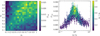 |
Fig. 5 Left: Pcap as a function of q2 and q3. Right: Pcap as a function of q2/q3. For that, we used m1 = 45 m⊙, a = aGW, and assumed a metal-poor cluster with Mcl = 5 × 10⁵ m⊙ and rh = 1 pc. The error bars are computed via |

5.3 Differential merger rates
A GC can be characterised by its Mcl, rh and metallicity. The metallicity affects mostly the properties of the BH mass function, while Mcl and rh determine the GW signature.
The mass ratio of merging BBHs, q, also depends on the GC properties. In this section we explore how the merger rate, R, depends on the mass ratio q, that is, dR/dq, and we derive a theoretical prediction for it.
Binary-single interactions can lead to mergers between BHs 1-2, 1-3 and 2-3, as the result of both GW captures and inspirals in between resonant interactions (hereafter referred to as inspirals). As we will later see, the majority of mergers come from inspirals between the BHs that constitute the initial binary (with mass ratio q = q2). Hence, for the purpose of this derivation, we approximate all mergers to come from this channel.
Under the assumption that there is a single BBH at any time, the differential merger rate can be written as
 (26)
(26)
where Γb(m1, q) is the mass-dependent binary formation rate and p2(q) is the probability that a dynamical binary has mass ratio q (see Section 4). Γb(m1, q) is the inverse of the time that it takes for the BBH to harden from the hard-soft boundary to aGW. From Hénon’s principle it follows that
 (27)
(27)
By integrating this differential equation from ahs to aGW we obtain
 (28)
(28)
where we assumed aGW ≪; ahs and the explicit value of aGW is given in Equation (17) such that
 (29)
(29)

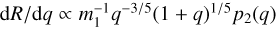
Note that the previous equation can be approximated by
 (31)
(31)
with α the exponent of the BH mass function. Because Mcl and rh only enter into Equation (30) through  in the constant of proportionality, the shape of dR/dq is entirely determined by the shape of the BH mass function, which is a function of metallicity and the stellar initial mass function. This means that the observed dR/dq of dynamically formed BBH can be used to infer the underlying BH mass function.
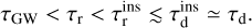
We now compare the result from Equation (30) to the differential rates that were found combining our scattering events with our GC model. The exact methodology used to obtain dR/dq from the scattering experiments is described in Appendix B. Contrary to Equation (30), here we take mergers from both GW captures and inspirals into account, involving BHs 1-2, 1-3 and 2-3. We can see in Fig. 6 the results formetal-poorandmetal-rich clusters, along with their respective predictions from Equation (30). The results from the scattering experiments for both metallicities agree with the result of Equation (30). We previously assumed that the majority of mergers involve the two BHs that were in the initial binary. Here we quantify this: approximately 70% of mergers are between BH 1 and 2; 20% are between BH 1 and 3 and mergers between the BH 2 and BH 3 contribute around 10%.
As seen in Fig. 6, for equal Mcl and rh, metal-rich clusters exhibit a higher rate of mergers than metal-poor clusters, by about a factor 2. This is to be expected from Hénon’s principle. A cluster requires its central BBH to provide a fixed quantity of energy per unit of time, independently of the characteristics of the BBH. A metal-rich cluster hosts a less massive central BBH, and to keep up with the energy demand of the cluster, the central BBH needs to shrink its orbit at a faster rate, leading to a quicker coalescence. This is explicitly seen in Equation (29) ( ). We adopted a primary mass for the metal-rich cluster that was half that of the metal-poor clusters, increasing the rate. In addition, the steeper BH mass function at higher metallicity (α = −2.3 vs. α = ࢤ0.5) results in binaries with lower q, preferentially increasing the rates at low q.
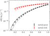 |
Fig. 6 Mass-ratio distribution of in-cluster mergers, for a metalpoor (black) and metal-rich (red) clusters with Mcl = 2 × 10⁵ m⊙ and rh = 3 pc. The dashed lines represent the theoretical slopes given in Equation (30) and the dotted lines represent p2(q2). Both the dashed and dotted lines have been normalised to the same normalisation constant as the data points. |
5.4 Rate of mergers
By integrating the differential rates shown in Fig. 6, we obtain the total rates that are expected for clusters with Mcl = 2 × 10⁵ M⊙ and rh = 3 pc, that is, typical values of GCs. This results in Rmr = 3.7 Gyrࢤ1, and Rmp = 1.5 Gyrࢤ1, for the metal-rich and metal-poor cluster, respectively.
These rates were computed using a distribution of m2 and m3. To estimate the effect of considering unequal masses, we also compute these rates assuming all interactions to happen among BHs of equal masses. That is, we use p2(q2) = δ(1 - q2) and p3(q3) = δ(1 - q3) (therefore, all masses involved in the three-body problem are equal to the primary mass). The resulting equal-mass rates are REM,mr = 3.5Gyrࢤ1 and REM,mp = 1.5 Gyrࢤ1 . These values are within a 5% of the unequal-mass rates shown above, which implies that the equal-mass assumption is a good approximation of the more realistic unequal-mass case. Nonetheless, this approximation is good as long as the involved masses are all equal to the primary mass, which is considered the highest mass in the cluster.
We now present the rate of mergers that is expected from a Milky Way-like GC population. We sample Mcl and rh from the log-normal distributions
 (32)
(32)
 (33)
with
(33)
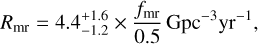
with  the half-mass density, μρ = 5 × 10² M⊙pcࢤ3, σρ = 0.75, μM = 2 × 10⁵ M⊙, σM = 0.5, and with the limits Mcl ∈ [102, 107] M⊙ and ρh > 0. For a number density of GCs in the Universe of 4 × 10⁹Gpc−3 (Antonini & Gieles 2020a), we obtain
 (34)
(34)
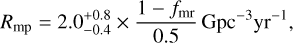 (35)
(35)
where fmr is the fraction of metal-rich clusters. For this computation, we sampled 1000 different clusters, and to save computation time we used the equal-mass approximation.
5.5 Inspirals driven by direct encounters
As explained in Section 5.2, inspirals happen when the binary has an eccentricity sufficiently high so that the timescale of merger is shorter than the timescale between resonant interactions. As considered in Antonini & Gieles (2020b), these high eccentricities can be achieved when, after a resonant interaction, the post-encounter eccentricity has a value above eGW. Nonetheless, in our simulations only around 60% of the inspiraled BBHs achieved their high e through this channel. The remaining 40% achieved it after a direct (i.e. non-resonant) encounter. As described in Heggie & Rasio (1996), direct encounters can modify the binary’s eccentricity, both positively and negatively, while the energy change is negligible. For a binary that is just below the critical eccentricity, this can cause a positive change in its eccentricity, potentially pushing it into an inspiral. This mechanism is referred to as a direct inspiral (Trani et al. 2024). Given how frequent direct encounters are in comparison to resonances, these two channels end up producing approximately the same number of inspirals.
Fig. 7 represents the initial (e0) and final (ef) eccentricities of the subset of binaries from our scattering experiments that undergo a direct inspiral. These inspirals can happen for field BHs that approach the binary with a distance of up to ~10a0, but the further away the approach, the closer e0 has to be to eGW in order for the binary to inspiral. For distances below ~3a0, some inspirals happen with ef above the solid line. For these close encounters, the binary’s SMA decreases after the encounter, changing eGW to lower values. For this subset of close encounters, what drives the inspiral is not only the increase in eccentricity, but also the decrease of the SMA. In Appendix C, we derive an approximation of the cross-section of direct inspirals ( ), and we compare it to the cross-section of inspirals coming from resonances (
 ). We find a ratio of
 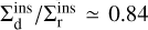 , reasonably close to the experimental ratio of around 2/3.
Most direct inspirals were found to happen in interactions with an inclination of θ ~ π/2. This is expected from Equation (15) of Heggie & Rasio (1996), which states that δe ∞ sin2θ, therefore maximising the changes in eccentricity when θ = π/2. In addition, direct inspirals may have a different eccentricity signature than inspirals coming from resonant interactions.
Direct inspirals arenotincludedin fastmodels for dynamical production of BBH inspirals, such as CBHBD (Antonini et al. 2023). There is currently a gap in the prediction of in-cluster mergers between these fast models and more accurate N-body models (Rastello et al. 2018; Kremer et al. 2020; Banerjee 2021; Barber et al. 2024), where the latter finds a higher proportion of BBHs coalescing inside the cluster relative to coalescences that occur after BBHs are ejected. Marín Pina & Gieles (2024) suggest that the aforementioned fast models lack an important ingredient which may compensate for the lack of in-cluster mergers, namely interactions between the dynamically active BBH and wide BBHs that form dynamically at a high rate. Direct inspirals provides an additional ingredient to bridge the gap between fast models and N-body simulations. Additionally, Monte Carlo codes analogous to the one described in Fregeau & Rasio (2007) account for direct encounters, but only if they are also strong encounters. This may overlook direct inspirals that occur during weak encounters, which are possible, as shown in Fig. 7.
So far, we have only considered BHs as the perturbers that trigger these direct inspirals. As it can be seen in Equation (C.3),  . This implies that the cross-section for direct inspiral decreases rapidly for lower mass perturbers. Namely, for stars, m3 decreases by around a factor ≳20, from ⟨m3⟩ ≃ 10 M⊙ for BHs, to ⟨m3⟩ ≃ 0.5 M⊙ for stars, which implies that
  decreases by a factor ≳150. In order for stars to become relevant perturbers, their number density should surpass that of BHs by around that factor, which is very unlikely in the core of a GC.
According to Heggie & Rasio (1996), the cross-section for a change in eccentricity δe is symmetric with respect to the sign of δe. This symmetry implies that both eccentricity excitation and de-excitation are equally possible. Note that, so far, we have focused on the possibility of BBHs inspiraling due to an eccentricity increase through a direct encounter, but there is also the possibility of the opposite to happen. What if, through eccentricity de-excitation, direct encounters prevent BBHs from coalescing?
Here, we argue why we believe this is unlikely. Let us consider a BBH in the process of inspiraling (that is, with e > eGW). By definition, this binary fulfils τGW < τr, with τGW the upper limit of the remaining lifetime of the BBH, and τr the timescale between resonant interactions. Using again the symmetry argument in the sign of δe, we approximate the cross-section of a direct inspiral (with timescale  ) to be the same as the cross-section of a direct encounter to decrease the eccentricity of a BBH with e > eGW to lower values (a coalescence prevention, with timescale τd). Therefore,
  . As mentioned previously, we find in our scattering experiments that
  , hence
  . Inthis last step, we just assumed that timescales and cross-sections are inversely proportional. Moreover, mergers caused by resonant interactions are only a subset of all resonant interactions. Consequently, τr is shorter than
  . Summarising, we have
 (36)
(36)
In other words, τGW < τd implies that, by the time a direct encounter arrives to prevent the coalescence, it is already too late.
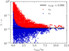 |
Fig. 7 Eccentricity of the subset of binaries that undergo direct inspiral, as a function of the minimum distance at which the field BH approaches one of the two components of the binary rmin. In red, the initial eccentricity, and in blue, the final eccentricity. The solid line represents the critical eccentricity eGW, calculated with Mcl = 5 × 10⁵ m⊙, rh = 1pc and α = ࢤ0.5. The binary has equal-mass components with m12 = 40M⊙, a SMA of 0.5 AU, and the field BH has a mass in the range m3 ∈ [0.1,0.5]m12. |
6 Discussion
Our model is similar to that of Antonini & Gieles (2020b), and we add the variations of the two mass ratios that are involved in binary-single interactions. In this section we describe the ingredients that are missing in our analysis.
6.1 Missing ingredients
We did not include evolutionary effects such as GC mass loss and the dynamical ejection of BH. This means that the BH mass function is always fully populated. This biases our mergers to low q, because in an evolving GC, the most massive BHs gradually get ejected from the GC and are therefore no longer available formergers. This is more important for metal-rich GCs that start with a lower m1 and eject BHs at a faster rate. Moreover, we assumed the presence of a single BBH in the core of our GC that only interacts with single BHs. The assumption of a single BBH is supported by results of N-body simulations (Marín Pina & Gieles 2024), but the authors also show that there is a high rate of interactions between the hard BBH and shorted-lived (soft) BBHs. In addition, a large fraction of primordial massive binaries is expected to turn into BBHs, that can interacts with the dynamical BBHs (Barber et al. 2024). Although less frequent, binary-binary interactions are estimated to contribute 25–45% of all highly eccentric mergers (Zevin et al. 2019; Marín Pina et al. 2025). Including them may change our analysis in a way that has not been explored.
Additionally, we only consider first generation mergers, that is, we do not consider mergers where at least one of the BHs has merged previously, referred to as hierarchical mergers. According to Ye & Fishbach (2024), hierarchical mergers approximately account for ~20% of mergers and may populate the pair-instability mass gap (Antonini et al. 2023). In order to account for hierarchical mergers, GW kicks must be taken into account. Due to linear momentum conservation, the post-merger BH receives a GW kick that, depending on q and the BH spins, can go from zero for non-spinning BHs with q = 1, to several hundreds-thousands of km/s, which is enough to eject the postmerger BH from the cluster (Antonini & Rasio 2016). Therefore, we should expect hierarchical mergers to have a higher relevance in clusters with a high vesc, where post-merger BHs are more likely to be retained in the cluster. It is for this reason that we expect the results from Section 5.3 to be more accurate for GCs of low vesc. In clusters where hierarchical mergers are indeed relevant, the post-merger BH, with mass ≲m1 + m2, eventually falls back to the cluster’s core and forms a new binary with the second-heaviest object in the cluster. Consequently, this second generation binary is likely to have a lower mass ratio than the previous first generation binary. As seen in Antonini et al. (2023), including hierarchical mergers increases the number of mergers at lower mass ratios.
6.2 Newtonian dynamics
The simulations were carried out using Newtonian dynamics, which allows us to determine the dynamics of the system not by the absolute masses, but rather by the mass ratios. This reduces the dimension of the parameter space by one and simplifies the analysis, but it does so at the cost of accuracy during close encounters (Gültekin et al. 2006). Therefore, our method to determine GW captures is only a rough approximation. Nevertheless, in-cluster coalescences are dominated by inspirals (Rodriguez et al. 2018; Antonini & Gieles 2020b), which in our model are predicted not by close approaches during resonant encounters, but by the semi-major axes and eccentricities attained after them, which are less sensitive to post-Newtonian terms. Therefore, the lack of post-Newtonian terms may affect primarily GW captures, which are subdominant with respect to inspirals. In addition, in Appendix D we find 1st order postNewtonian effects are safe to ignore in the specific case of direct inspirals.
7 Conclusions
In this study, we have investigated unequal-mass binary-single interactions in the Newtonian point-mass limit. For that, we have simulated a total of O(107) scattering events using STARLAB. Our key findings are:
The fractional change of binding energy following a resonant interaction, Δr, can be well described by Δr = 0.2 [1 - exp(-Am3/m12)] with A ≃ 7.0 for m3 < m12;
The number of intermediate states peaks at NIMS ≃ 20 if the two lightest bodies in the triplet have similar masses (m2 ≃ m3). Outside of this regime, NIMS drops considerably, reducing the probability for GW captures;
In agreement with Stone & Leigh (2019), we found a mildly superthermal distribution of eccentricities near the equalmass case with high angular momentum. Outside of the equal-mass case and considering lower m3, the eccentricity distribution after resonant interactions is closer to thermal.
We used our scattering experiments in combination with a model for the evolution of a BBH in a GC to explore the GW implications of unequal-mass encounters of BHs in GCs. We summarise the main results below.
The differential merger rate for different mass ratios is
 , with p2(q) the mass-ratio distribution of dynamically formed BBHs, which depends on the underlying BH mass function. For a power-law BH mass function with index α, this can be well approximated by
  . This means that the mass-ratio distribution of mergers is slightly flatter than the mass-ratio distribution of the dynamical binaries (∞ q3.5+α);
In equal conditions of cluster mass and radius, metal-rich clusters have approximately double the merger rate as metalpoor clusters;
We compared the rate of mergers obtained assuming both the equal and the unequal-mass regimes, and found that the equal-mass case can approximate within a 5 %error the rates predicted by the latter, as long as the chosen masses are equal to the primary mass;
While BBHs inspiral when their eccentricity is above a threshold eGW(a) (according to our model), only 60% of the inspiraled BBHs were found to attain their high eccentricities through resonant interactions. The other 40% obtained their high eccentricity after a direct encounter. This mechanism was denominated as direct inspirals, and its contribution to mergers may be the missing ingredient that bridges the current gap between fast models and more accurate N-body models.
Acknowledgements
B.R.F., D.M.P. and M.G. acknowledge financial support from the grants PID2021-125485NB-C22, EUR2020-112157, CEX2019-000918- M funded by MCIN/AEI/10.13039/501100011033 (State Agency for Research of the Spanish Ministry of Science and Innovation) and SGR-2021-01069 (AGAUR). B.R.F. thanks the Leiden Observatory, where part of this work was done, for their hospitality during a three months research stay.
Appendix A Cross-sections
Analogously to particle physics, we can study binary-single interactions using cross-sections. We define the cross-section for an event X to happen as
 (A.1)
(A.1)
where PX is the fraction of interactions with an impact parameter b < bmax that undergo an outcome X (e.g. resonant, exchange, etc.). When bmax → ∞, nearly all interactions are distant flybys that do not perturb the binary, making PX →; 0 such that  converges5. In practice, bmax is an infrared cutoff chosen to be sufficiently large so that ΣX converges. The choice of bmax is described in Section 2.2. The average energy change of the binary, ⟨Δ⟩ (equation 4), depends on the arbitrary choice of bmax, making it an ill-defined quantity. Because resonant interactions only occur within a finite bmax, the mean value of Δr (obtained in Section 3.1) is a well-defined quantity. Furthermore, given a cross-section
  , one can compute the rate RX at which encounters of type X happen between the binary and its surrounding bodies:
 (A.2)
(A.2)
where n is the density of the surrounding bodies.
When computing cross-sections, there are two sources of errors (Hut & Bahcall 1983). The first is the statistical error present in all probabilistic processes, given by
 (A.3)
(A.3)
where NX is the number of interactions of type X. The second source of error comes from the computation: to keep in check this source of numerical inaccuracies, the integration steps must be kept small enough. As it is stated in Section 2.2, the error in the total energy of the system is kept under control, hence making the systematic errors that come from numerical inaccuracies negligible, much less than 1 % (McMillan & Hut 1996). It is difficult to have a measure of the computational error, so we conservatively assume it is equal to the statistical error. In addition, our definition of a minimum in s2 (Section 2.1) is a source of error when classifying events as resonant or non-resonant. This source of error is again difficult to estimate analytically, and as a first approximation it is considered to be within the computational error.
Appendix B Derivation of dR/dq from the scattering experiments
Here we show how we obtain the differential merger rate, dR/dq, for a GC with arbitrary Mcl, rh and metallicity based on the results of the gravitational scattering experiments presented in Section 3. According to Hénon’s principle, the rate at which the central BBH releases energy is determined by the cluster, and is independent of the BBH’s properties. Assuming the binary only releases its energy through resonant binary-single interactions, this rate can be expressed as (see Section 5.2)
 (B.1)
(B.1)
We define Rr ≡ 1/τr as the rate at which the BBH undergoes resonant interactions. The rate at which BHs i and j coalesce, denoted by rij, is Rr times the number of mergers per resonant interaction, which is obtained via
 (B.2)
(B.2)
where  and
and  are the cross-sections for i − j mergers and resonant interactions respectively. We find ⟨Δr⟩ from
![$\langle\Delta_{\rm r}\rangle = \int_{m_{\rm min}}^{m_{\rm max}}\Delta_0\left[1- {\rm exp}\left(-A\frac{m_3}{m_{12}}\right)\right]p_3(m_3) {\rm d}m_3,$](/articles/aa/full_html/2025/05/aa50890-24/aa50890-24-eq90.png) (B.3)
(B.3)
where we use the fitting function given in Equation (5), and p3(m3) is given in Section 4.2. We assume a pre-existing BBH with mass ratio q2, and an interaction with a single BH of mass ratio q3. It is for this reason that equation (B.2) must be weighed by p2(q2) and p3(q3), given in Section 4.2. Therefore
 (B.4)
(B.4)
The ratio  is obtained from our binary-single scattering events, which are described in Section 2.2. In our simulations we use values of q2 and q3 in the range [0.1,1] and spaced in steps of 0.05. We perform the following steps:
Determine the primary mass (and mass scale) m1, equal to 25 M⊙ for metal-rich clusters, and 50 M⊙ for metal-poor clusters (see Section 4.2),
Select one of the 19 values of q2 that were used in the simulations and determine the secondary mass m2 = m1 q2, and select one of the 19 values of q3 that were used in the simulations and determine the mass of the field BH m3 = m1 q3,
For all encounters with this combination of q2 and q3 , compute Σr from equation (A.1).
Sample the SMA of the binary from pa(a), with a ∈ [am, ahs] (see Section 4.3),
For all encounters with this combination of q2, q3 and a, compute
 , including both GW captures and inspirals. A GW capture between BHs i and j happens if the minimum distance between them that is reached during the whole encounter is below rGW (see Section 5.1). An inspiral between BHs i and j happens if the final BBH is composed by these two BHs, and has an eccentricity after the interaction that is above eGW (see Section 5.2).
Steps 4 and 5 are repeated for 10 randomly sampled SMAs, obtaining the ratio  averaged over a, and steps 2 to 5 are repeated for all values of q2 and q3, thus obtaining
  . We can now use equation (B.4) to determine dR/dq. Let us first consider mergers among BHs 1 and 2. For these mergers, q = q2. In order to obtain dR12/dq, we have to integrate over all possible q3’s
 (B.5)
(B.5)
Similarly, for mergers between BHs 1 and 3, we have q = q3, and for mergers between BHs 2 and 3, we have q = min(q2, q3)/max(q2, q3). To obtain their respective differential rates, we integrate along lines of constant q, as in the previous equation. The differential rate that includes all types of mergers is
 (B.6)
(B.6)
The results of this exercise are shown in Fig. 6.
Appendix C Derivation of 
Here, we compute the ratio between the cross-section of a direct inspiral  and that of a resonant inspiral
  . First, we estimate
  with
with
 (C.1)
(C.1)
where  , and
, and  is the cross-section of resonant interactions
 (C.2)
(C.2)
where A is set to a value of 19.55 by integrating Equation (24) from Heggie & Hut (1993). For a binary of initial eccentricity e, the cross-section for a direct encounter to change the eccentricity by a value δe > δe0 is given by Heggie & Rasio (1996)
 (C.3)
(C.3)
This expression assumes rp ≫ a. Although in Fig. 7 it can be seen that a big proportion of inspirals happen at rp ≃ a, our aim is not to obtain an exact value of  , but rather to understand how it behaves relative to
  . It is for this reason that, even though the assumption rp ≫ a is not always met, we still use equation (C.3).
To know the cross-section for δe to be high enough to trigger an inspiral, we set δe0 = eGW - e. Now, we set  to be the expected value of Σ (δe > δe0) over all possible initial eccentricities:
 (C.4)
(C.4)
where we have assumed pe(e) to be a thermal distribution with e in the range e ∈ [0, eGW]. For equal masses, the ratio of crosssections reduces to
 (C.5)
(C.5)
where eGW = eGW(a), and we define the integral
 (C.6)
(C.6)
If most inspirals happen at a ≃ aGW, then
 (C.7)
(C.7)
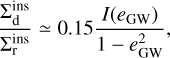
This result is reasonably close to the ratio observed in our simulations, which is 2/3: indeed, both cross-sections are of the same order of magnitude. From equation (C.5) and Equation (25) it can be seen that the ratio of cross-sections scales with  , where we neglect the weak dependence that I(eGW) has on eGW. This suggests that the relative importance of direct encounters increases for softer binaries.
Appendix D The effect of 1pN precession on direct inspirals
Here, we estimate whether ignoring 1st order post-Newtonian terms is a good approximation for the specific case of direct inspirals. For that, we compare the timescale at which the BBH precesses, τω, to the timescale at which the dimensionless angular momentum of the binary l changes due to the field BH, τl. If τl < τω, then it is safe to ignore relativistic precession. We can express both timescales as  and
and  , with
 (D.1)
(D.1)
where T is the orbital period of the BBH,  the rate at which the perihelion shifts, and Δω the perihelion shift during one orbital period. From this it follows that
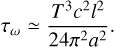 (D.2)
(D.2)
We proceed now with tl. We can express  as
as
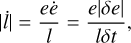 (D.3)
(D.3)
with δe the change of eccentricity over a time δt. After Heggie & Rasio (1996), δe after a direct encounter is
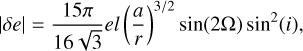 (D.4)
(D.4)
where Ω is the longitude of the ascending node, and we assume equal masses. For the specific case of direct inspirals, the conditions are such that δe is maximised, implying sin(2Ω) ~ sin(i) ~ 1. Using  we are left with
 (D.5)
(D.5)
We can now perform the ratio τl/τω, given by
 (D.6)
(D.6)
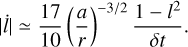
where we use the fact that δt scales with r as δt ~ T(r/a)3/2, and we use Kepler’s third law to write T in units a. Note that precession becomes increasingly important as a shrinks. We place ourselves in the worst case scenario by adopting its minimum value a = aGW, given in Section 4.3. For that, we use a cluster with Mcl = 2 × 10⁵ M⊙, and rh = 3 pc. In the particular case of direct inspirals, we assume l to be close to the threshold lGW, given in Section 5.2. Therefore
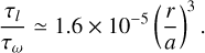 (D.7)
(D.7)
By imposing τl < τω we obtain
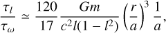 (D.8)
(D.8)
Consequently, even for the smallest possible SMA, precession is unimportant for all flybys with distance r < 18a. In our scattering experiments, we find that all direct inspirals happen for r < 12a (see Fig. 7); therefore, it is safe to ignore the effect of precession.
References
- Abbott, B. P., LIGO Scientific Collaboration, & Virgo Collaboration 2016, Phys. Rev. Lett., 116, 061102 [Google Scholar]
- Abbott, R., The LIGO Scientific Collaboration, the Virgo Collaboration, & the KAGRA Collaboration 2021, arXiv e-prints [arXiv:2111.03606] [Google Scholar]
- Alexander, P. E. R., & Gieles, M. 2012, MNRAS, 422, 3415 [NASA ADS] [CrossRef] [Google Scholar]
- Antonini, F., & Gieles, M. 2020a, Phys. Rev. D, 102, 123016 [NASA ADS] [CrossRef] [Google Scholar]
- Antonini, F., & Gieles, M. 2020b, MNRAS, 492, 2936 [CrossRef] [Google Scholar]
- Antonini, F., & Rasio, F. A. 2016, ApJ, 831, 187 [Google Scholar]
- Antonini, F., Gieles, M., Dosopoulou, F., & Chattopadhyay, D. 2023, MNRAS, 522, 466 [NASA ADS] [CrossRef] [Google Scholar]
- Banerjee, S. 2018, MNRAS, 481, 5123 [NASA ADS] [CrossRef] [Google Scholar]
- Banerjee, S. 2021, MNRAS, 503, 3371 [NASA ADS] [CrossRef] [Google Scholar]
- Banerjee, S., Belczynski, K., Fryer, C. L., et al. 2020, A&A, 639, A41 [NASA ADS] [CrossRef] [EDP Sciences] [Google Scholar]
- Barber, j., Chattopadhyay, D., & Antonini, F. 2024, MNRAS, 527, 7363 [Google Scholar]
- Breen, P. G., & Heggie, D. C. 2013, MNRAS, 432, 2779 [NASA ADS] [CrossRef] [Google Scholar]
- Chazy, j. 1929, j. Math. Pures Appl., 8, 353 [Google Scholar]
- Di Carlo, U. N., Giacobbo, N., Mapelli, M., et al. 2019, MNRAS, 487, 2947 [NASA ADS] [CrossRef] [Google Scholar]
- Fabj, G., & Samsing, j. 2024, MNRAS, 535, 3630 [Google Scholar]
- Fregeau, j. M., & Rasio, F. A. 2007, ApJ, 658, 1047 [Google Scholar]
- Fregeau, j. M., Cheung, P., Portegies Zwart, S. F., & Rasio, F. A. 2004, MNRAS, 352, 1 [CrossRef] [Google Scholar]
- Gieles, M., Heggie, D., & Zhao, H. 2011, MNRAS, 413, 2509 [Google Scholar]
- Ginat, Y. B., & Perets, H. B. 2023, MNRAS, 519, L15 [Google Scholar]
- Gültekin, K., Miller, M. C., & Hamilton, D. P. 2006, ApJ, 640, 156 [CrossRef] [Google Scholar]
- Hansen, R. O. 1972, Phys. Rev. D, 5, 1021 [NASA ADS] [CrossRef] [Google Scholar]
- Heggie, D. C. 1975, MNRAS, 173, 729 [NASA ADS] [CrossRef] [Google Scholar]
- Heggie, D. C., & Hut, P. 1993, ApJS, 85, 347 [NASA ADS] [CrossRef] [Google Scholar]
- Heggie, D., & Hut, P. 2003, The Gravitational Million-Body Problem: a Multidisciplinary Approach to Star Cluster Dynamics (Cambridge: Cambridge University Press) [CrossRef] [Google Scholar]
- Heggie, D. C., & Rasio, F. A. 1996, MNRAS, 282, 1064 [NASA ADS] [CrossRef] [Google Scholar]
- Heggie, D. C., Hut, P., & McMillan, S. L. W. 1996, ApJ, 467, 359 [Google Scholar]
- Hénon, M. 1961, Annales d’Astrophysique, 24, 369 [NASA ADS] [Google Scholar]
- Hénon, M. 1975, IAU Symp., 69, 133 [Google Scholar]
- Hills, j. G., & Fullerton, L. W. 1980, AJ, 85, 1281 [NASA ADS] [CrossRef] [Google Scholar]
- Hurley, j. R., Pols, O. R., & Tout, C. A. 2000, MNRAS, 315, 543 [Google Scholar]
- Hut, P., & Bahcall, j. N. 1983, ApJ, 268, 319 [NASA ADS] [CrossRef] [Google Scholar]
- Hut, P., Makino, j., & McMillan, S. 1995, ApJ, 443, L93 [NASA ADS] [CrossRef] [Google Scholar]
- Jeans, j. H. 1919, MNRAS, 79, 408 [NASA ADS] [CrossRef] [Google Scholar]
- King, i. R. 1966, AJ, 71, 64 [Google Scholar]
- Kremer, K., Ye, C. S., Rui, N. Z., et al. 2020, ApJS, 247, 48 [NASA ADS] [CrossRef] [Google Scholar]
- Makino, j., & Aarseth, S. j. 1992, PASJ, 44, 141 [Google Scholar]
- Mandel, i., & Broekgaarden, F. S. 2022, Liv. Rev. Relativ., 25, 1 [NASA ADS] [CrossRef] [Google Scholar]
- Marín Pina, D., & Gieles, M. 2024, MNRAS, 527, 8369 [Google Scholar]
- Marín Pina, D., Gieles, M., Andrade, T., & Trani, A. A. 2025, A&A, submitted [arXiv:2501.02907] [NASA ADS] [CrossRef] [EDP Sciences] [Google Scholar]
- McMillan, S. L. W., & Hut, P. 1996, ApJ, 467, 348 [CrossRef] [Google Scholar]
- Peters, P. C. 1964, Phys. Rev., 136, B1224 [Google Scholar]
- Portegies Zwart, S. F., & McMillan, S. L. W. 2000, ApJ, 528, L17 [Google Scholar]
- Portegies Zwart, S., Gaburov, E., Chen, H.-C., & Gürkan, M. A. 2007, MNRAS, 378, L29 [Google Scholar]
- Portegies Zwart, S. F., McMillan, S. L. W., & Gieles, M. 2010, ARA&A, 48, 431 [NASA ADS] [CrossRef] [Google Scholar]
- Quinlan, G. D. 1996, New A, 1, 35 [NASA ADS] [CrossRef] [Google Scholar]
- Rastello, S., Amaro-Seoane, P., Arca-Sedda, M., et al. 2018, MNRAS, 483, 1233 [Google Scholar]
- Rodriguez, C. L., Morscher, M., Pattabiraman, B., et al. 2015, Phys. Rev. Lett., 115, 051101 [Google Scholar]
- Rodriguez, C. L., Chatterjee, S., & Rasio, F. A. 2016, Phys. Rev. D, 93, 084029 [NASA ADS] [CrossRef] [Google Scholar]
- Rodriguez, C. L., Amaro-Seoane, P., Chatterjee, S., et al. 2018, Phys. Rev. D, 98, 123005 [NASA ADS] [CrossRef] [Google Scholar]
- Samsing, j. 2018, Phys. Rev. D, 97, 103014 [CrossRef] [Google Scholar]
- Samsing, j., MacLeod, M., & Ramirez-Ruiz, E. 2014, ApJ, 784, 71 [NASA ADS] [CrossRef] [Google Scholar]
- Samsing, j., D’Orazio, D. j., Kremer, K., Rodriguez, C. L., & Askar, A. 2020, Phys. Rev. D, 101, 123010 [Google Scholar]
- Sigurdsson, S., & Phinney, E. S. 1993, ApJ, 415, 631 [NASA ADS] [CrossRef] [Google Scholar]
- Spitzer, L. 1987, Dynamical Evolution of Globular Clusters (Princeton: Princeton University Press) [Google Scholar]
- Spitzer, Lyman, j., & Hart, M. H. 1971, ApJ, 164, 399 [NASA ADS] [CrossRef] [Google Scholar]
- Stone, N. C., & Leigh, N. W. C. 2019, Nature, 576, 406 [NASA ADS] [CrossRef] [Google Scholar]
- Trani, A. A., Leigh, N. W. C., Boekholt, T. C. N., & Portegies Zwart, S. 2024, A&A, 689, A24 [NASA ADS] [CrossRef] [EDP Sciences] [Google Scholar]
- Ye, C. S., & Fishbach, M. 2024, ApJ, 967, 1 [Google Scholar]
- Zevin, M., Samsing, j., Rodriguez, C., Haster, C.-J., & Ramirez-Ruiz, E. 2019, ApJ, 871, 91 [NASA ADS] [CrossRef] [Google Scholar]
We note that this flattening was not considered by Antonini & Gieles (2020b).

All Tables
Parameters needed to specify the initial conditions of a scattering simulation, including their corresponding ranges and the distributions.
All Figures
|
Fig. 1 ⟨Δr⟩, in units of Δ0, as a function of m3/m12. Each data point represents a different combination of q2 and q3. The solid line is the fitted function. |
| In the text | |
|
Fig. 2 Left: ⟨NIMS⟩ for resonant encounters with different mass ratios. Right: ⟨NIMS⟩ for resonant encounters, as a function of q3/q2. The error bars correspond to V2 times the standard error of the mean. |
| In the text | |
|
Fig. 3 Left: theoretical ⟨NIMS⟩ for resonant encounters with different mass ratios. Right: theoretical ⟨NIMS⟩ for resonant encounters, as a function of q3/q2. |
| In the text | |
|
Fig. 4 Eccentricity distribution after a democratic resonance. For the approximate equal mass case, the data points were selected by imposing the condition q2, q3 ∈ [0.5,1]. For the unequal-mass case, the data points were selected by imposing the condition q2 ∈ [0.1,0.4] or q3 ∈ [0.1,0.4]. The dashed lines represent the thermal distribution, and the solid line represents the mildly superthermal distribution. |
| In the text | |
|
Fig. 5 Left: Pcap as a function of q2 and q3. Right: Pcap as a function of q2/q3. For that, we used m1 = 45 m⊙, a = aGW, and assumed a metal-poor cluster with Mcl = 5 × 10⁵ m⊙ and rh = 1 pc. The error bars are computed via |
| In the text | |
|
Fig. 6 Mass-ratio distribution of in-cluster mergers, for a metalpoor (black) and metal-rich (red) clusters with Mcl = 2 × 10⁵ m⊙ and rh = 3 pc. The dashed lines represent the theoretical slopes given in Equation (30) and the dotted lines represent p2(q2). Both the dashed and dotted lines have been normalised to the same normalisation constant as the data points. |
| In the text | |
|
Fig. 7 Eccentricity of the subset of binaries that undergo direct inspiral, as a function of the minimum distance at which the field BH approaches one of the two components of the binary rmin. In red, the initial eccentricity, and in blue, the final eccentricity. The solid line represents the critical eccentricity eGW, calculated with Mcl = 5 × 10⁵ m⊙, rh = 1pc and α = ࢤ0.5. The binary has equal-mass components with m12 = 40M⊙, a SMA of 0.5 AU, and the field BH has a mass in the range m3 ∈ [0.1,0.5]m12. |
| In the text | |
Current usage metrics show cumulative count of Article Views (full-text article views including HTML views, PDF and ePub downloads, according to the available data) and Abstracts Views on Vision4Press platform.
Data correspond to usage on the plateform after 2015. The current usage metrics is available 48-96 hours after online publication and is updated daily on week days.
Initial download of the metrics may take a while.