| Issue |
A&A
Volume 693, January 2025
|
|
|---|---|---|
| Article Number | A3 | |
| Number of page(s) | 13 | |
| Section | Galactic structure, stellar clusters and populations | |
| DOI | https://doi.org/10.1051/0004-6361/202450868 | |
| Published online | 23 December 2024 | |
Constraints on the history of Galactic spiral arms revealed by Gaia GSP-Spec α-elements
1
Université Côte d’Azur, Observatoire de la Côte d’Azur, CNRS,
Laboratoire Lagrange,
France
2
Osservatorio Astrofisico di Torino, Istituto Nazionale di Astrofisica (INAF),
10025
Pino Torinese,
Italy
3
INAF Osservatorio Astronomico di Trieste,
via G.B. Tiepolo 11,
34131
Trieste,
Italy
4
Dipartimento di Fisica, Sezione di Astronomia, Università di Trieste,
Via G. B. Tiepolo 11,
34143
Trieste,
Italy
5
INFN, Sezione di Trieste,
Via A. Valerio 2,
34127
Trieste,
Italy
★ Corresponding author; mbarbillon@gmail.com
Received:
24
May
2024
Accepted:
8
November
2024
Context. The distribution of chemical elements in the Galactic disc can reveal fundamental clues on the physical processes that led to the current configuration of our Galaxy.
Aims. We aim to map chemical azimuthal variations in the Galactic disc using individual stellar chemical abundances, such as those of calcium and magnesium, and we discuss their possible connection with the spiral arms and other perturbing mechanisms.
Methods. Taking advantage of Gaia Data Release 3, we mapped [Ca/Fe] and [Mg/Fe] fluctuations in a region of about 4 kpc around the Sun using different samples of bright giant stars. We implemented a kernel density estimator technique to enhance the chemical inhomogeneities.
Results. We observed clear radial gradients and azimuthal fluctuations in the maps of α elements with respect to iron abundances for young (⪅150 Myr) and old (⪆2 Gyr) stellar populations, whose amplitudes depend on the considered chemical species. In the young population, stars within the spiral arms (mostly the Sagittarius-Carina arm and the upper part of the Local arm) are globally more metal-rich and calcium-rich (~0–0.19 dex) but more [Ca/Fe]-poor (~0.06 dex) and [Mg/Fe]-poor (~0.05 dex) than the stars in the inter-arm regions. This indicates higher enhancements in iron than in α elements within the spiral arms. This depletion in [α/Fe] is discussed in the context of different theoretical scenarios, and we compare it quantitatively to a 2D chemical evolution model that accounts for multiple spiral arm patterns. Interestingly, the [Ca/Fe] maps of the old population sample present clear deficiencies along a segment of the Local arm as traced by young populations. We caution that for this old sample, the quality of the obtained maps might be limited along a specific line of sight by the impact of the Gaia scanning law.
Conclusions. Our understanding of the chemical evolution of the disc changes from a simplistic 1D radial view to a more complete 2D perspective that combines radial and azimuthal trends and small-scale variations. This study has confirmed the importance of using individual chemical diagnostics as tracers of the spiral arms in disc galaxies. We suggest that the observed α-abundances should be accounted for by models and simulations when the spiral arm lifetimes are addresed.
Key words: Galaxy: abundances / Galaxy: disk / Galaxy: evolution / Galaxy: stellar content / Galaxy: structure
© The Authors 2024
 Open Access article, published by EDP Sciences, under the terms of the Creative Commons Attribution License (https://creativecommons.org/licenses/by/4.0), which permits unrestricted use, distribution, and reproduction in any medium, provided the original work is properly cited.
This article is published in open access under the Subscribe to Open model. Subscribe to A&A to support open access publication.
1 Introduction
The ability to map the structural, kinematic and chemical properties of stars in our Galaxy has revealed that the classical components of the Milky Way (MW), namely the disc(s) (composed of the thin and thick discs; Gilmore & Reid 1983), the bulge, and the halo, are interlinked and constitute a system that interacts with its environment (e.g. Helmi et al. 2018; Antoja et al. 2023). The accretion of satellite galaxies can leave important signatures in the Galactic disc (Purcell et al. 2011; Laporte et al. 2018; Bland-Hawthorn et al. 2019; Garavito-Camargo et al. 2021). Moreover, the large-scale spiral structures of the Galaxy (e.g. Georgelin & Georgelin 1976; Taylor & Cordes 1993; Reid et al. 2019; Minniti et al. 2021) and the central bar (e.g. Okuda et al. 1977; Palicio et al. 2018; Khoperskov et al. 2020; Gaia Collaboration 2023a) are expected to be crucial drivers of the dynamical evolution of disc stars (e.g. Schönrich & Binney 2009; Minchev et al. 2012; Hunt et al. 2019; Santos-Peral et al. 2021; Palicio et al. 2023, and others).
As a consequence of the dynamical mechanisms at work in the Galactic disc, the stellar kinematic history can be completely erased. On the other hand, the chemical composition will be preserved throughout the stellar life. In a galaxy with a radial metallicity gradient (Anders et al. 2017; Katz et al. 2021), any process of radial migration would give rise to chemical azimuthal variations.
To disentangle the dynamical history of Galactic stellar populations, it is crucial to map the spatial distribution of metals in the disc. In external disc galaxies, both radial and azimuthal chemical gradients have been mapped (Pilyugin et al. 2014; Vogt et al. 2017; Zurita et al. 2021). In the MW, chemical azimuthal variations have been found using HII regions (Balser et al. 2011; Wenger et al. 2019), Cepheids (Genovali et al. 2014; Kovtyukh et al. 2022), and the interstellar medium (De Cia et al. 2021), amongst others. With the advent of Gaia Data Release (DR) 3 (Gaia Collaboration 2023c), azimuthal variations were mapped in the metallicity of both young and old stars (Poggio et al. 2022; Gaia Collaboration 2023b; Hawkins 2023). More precisely, using young giants (⪅150 Myr), Poggio et al. (2022) mapped local metallicity enhancements at the level of ~0.1 dex, which appeared to be statistically correlated with the position of the nearest spiral arms in the Galaxy. Using giant stars in Gaia DR3, Hawkins (2023) detected azimuthal variations that appeared to be co-located with the spiral arms; however, using OBAF-type stars in the Large Sky Area Multi-Object Fibre Spectroscopic Telescope (LAMOST), they found that the correlation was not evident. Based on numerical simulations, spiral arms are expected to drive azimuthal variations in the disc metallicity (Grand et al. 2016; Khoperskov et al. 2018, 2023; Debattista et al. 2024). Moreover, azimuthal metallicity substructures can be caused by the radial migration induced by satellite galaxies (Carr et al. 2022) and/or the Galactic bar (Di Matteo et al. 2013; Filion et al. 2023).
This complexity reveals the need of further constraints on the structural and chemo-dynamical characteristics of the Galactic disc in both the radial and azimuthal dimensions.
Analytic chemical evolution models of the Galactic disc have so far ignored variations in the azimuthal surface density, with the recent exception of the 2D Spitoni et al. (2019, 2023) or Mollá et al. (2019) models. One of the main results of Spitoni et al. (2023) is that elements synthesised on short timescales, like α elements, exhibit stronger abundance fluctuations along the spiral arms than heavier elements such as iron (Fe) and barium (Ba), which are produced with a longer time delay. The aim of this study is a detailed analysis of the chemical inhomogeneities in the MW disc, with the goal of detecting the spiral arm signatures in calcium and magnesium, and more generally, to explore radial and azimuthal chemical variations in the disc.
In Sect. 2, we explain the details of our data selections and method. Section 3 describes our results, and Sect. 4 summarises our discussions and conclusions.
2 Data selection and method
To select tracers of stellar disc populations and map large-scale inhomogeneities in individual chemical abundances, we followed the procedure described in Poggio et al. (2022, hereafter referred to as Paper I). We used stellar atmospheric parameters (effective temperature Teff, surface gravity log(g), global metallicity [M/H]), calcium [Ca/Fe], and magnesium [Mg/Fe] abundances derived from Gaia RVS spectra by the General Stellar Parametriser-Spectroscopy (GSP − S pec1) module (Recio-Blanco et al. 2023). Each selected element abundance (except for the metallicity) was calibrated as a function of Teff using the polynomials from the end of Table 4 of Recio-Blanco et al. (2023), lately extended in Table A.1 of Recio-Blanco et al (2024) for the log(g) and the magnesium ratio. In addition, we used the geometric distances from Bailer-Jones et al. (2021) and the Galactic velocities calculated in Gaia Collaboration (2023b). We performed different quality selections in astrophysical parameters, astrometry, distances, and kinematics to minimise possible contaminants (cf. more details in Appendix A).
In this preliminary selection, we were particularly interested in selecting giant stars because they allowed us to sample a relatively large volume of the Galactic disc and to perform a robust statistical analysis based on the large number of high-quality chemical measurements. Specifically, we aimed to select two samples of typically young (relatively hotter) and old (relatively cooler) giants stars, hereafter labelled samples A and C, respectively. Following Paper I, we selected stars in the Kiel diagram using cuts in Teff and log(g) that created inclined boxes, as shown in Fig. 1, within the following limits:
log(g)_{uncalibrated} < 1.5 &
log(g)_{uncalib} > 0.5 &
(log(g)_{uncalib} > (coeff*teff + interc_left))&
(log(g)_{uncalib} < (coeff*teff + interc_right))&
abs(Z) < 0.75 kpc
where the adopted slope is coeff, and the intercepts delimit the selected regions for samples A and C (cf. Paper I). The surface gravity used here is the uncalibrated one, and Z is the distance to the Galactic plane. Compared to Paper I, we simply included greater constraints on [M/H] uncertainties by adding [α/Fe] uncertainties and individual abundance flags and considering calibrated parameters. In order to validate the robustness of the selected abundance statistics, we fixed a condition where the [X/Fe] uncertainty had to be twice higher than the standard deviation of the studied chemical species, σ[X/Fe].
We also imposed an additional temperature constraint, requiring Teff > 4200 K. As shown in Fig. 1, this cut is almost irrelevant for sample A, but it is very important for sample C (as it removes 211 524 stars). The Teff > 4200 K criterion aims to minimise selection function effects, as explained in the following. The scanning law of the Gaia satellite leaves strong signatures in the [α/Fe] abundance distribution of the Gaia GSP-Spec catalogue, as shown in Fig. 3 of Gaia Collaboration (2023b). After performing some tests, we found that the scanning law artefacts are particularly evident at high Galactic latitudes (cf. also Cantat-Gaudin et al. 2024), and they are quite evident for cooler stars (while hot stars tend to be more confined to the Galactic plane). By applying this Teff cut-off, we also limited the contribution of cooler stars, which are more difficult to parametrise. This helped us to reduce the scanning-law effects on the sample C α-abundances of this study, which is composed of cooler stars.
The process of obtaining the initial queries and the final samples is explained in Appendix A. In the end, sample A was preferentially populated by young stars (cold blue loop stars) that trace the spiral arms, while sample C contained older disc populations (red giant branch (RGB) stars). We constructed chemical maps based on the two samples selected in this section, with the goal of comparing two stellar populations of different ages.
Figure 1 shows the final selected area that defined sample A (blue dots) and sample C (red dots) with the initial selection (grey dots) as a visual reference. Sample A included 11 678 stars with [Ca/Fe] abundances and reached distances up to ~4 kpc around the Sun. It presents a median G magnitude of 11.40 mag (with 10.35 mag and 12.09 mag being the first and the third quartiles of the distribution, respectively). On the other hand, sample C included 74740 stars with [Ca/Fe] abundances. It reached distances up to ~4 kpc around the Sun. The G magnitude distribution spans from 11.40 mag (first quartile) to 10.44 mag (third quartile), with a median value of 12.06 mag. In addition, sample A contained about 689 stars with [Mg/Fe] abundances covering a smaller volume of the disc (~1.5 kpc around the Sun). For sample C, the condition we fixed to have the [Mg/Fe] uncertainty twice higher than the σ[Mg/Fe] was not achieved in the magnesium abundance. For this reason, we do not show the [Mg/Fe] abundance for this sample. The different characteristics of samples A and C are summarised in Table A.1, where the uncertainties of all parameters are defined as half of the difference between their upper and lower confidence levels, for example, Teffunc = [Teffupper-Tefflower]/2 (Recio-Blanco et al. 2023). We also checked the completeness of our dataset by comparing the spectral type classification2 of the Extended Stellar Parametrizer (ESP) catalogue (Creevey et al. 2023) against GSP-Spec, where the former is more complete to the faint magnitude range as it uses Gaia BP/RP spectra. With respect to the ESP catalogue, we obtained a completeness of 93% down to G < 12 mag for the entire query, and a completeness of 84% and 87% down to G < 12 mag for samples A and C, respectively.
In addition, as presented in Fig. 1, we estimated the typical age range within the selected portion of the Kiel diagram using BaSTI3,4 stellar isochrones (Hidalgo et al. 2018). It was shown that high-precision GSP-Spec data allow us to break the age-metallicity degeneracy along the giant branch (Recio-Blanco et al. 2024). To take the age-metallicity degeneracy into account, we used the value of the first quartile of the metallicity distribution ([M/H] = −0.32 ± 0.015 dex) for the hottest isochrone, and we used its third quartile ([M/H] = −0.14 ± 0.035 dex) for the coolest one for the youngest sample. Hence, varying the BaSTI age parameter to include the 90% density of our sample leads to an approximate age range between 30 and 130 Myr. Following a similar approach, we found that sample C contains stars older than 2 Gyr, with a first quartile of the metallicity distribution equal to [M/H] = −0.44 ± 0.015 dex for the hottest isochrone, and a third quartile of [M/H] = −0.20 ± 0.035 dex for the coolest one. We also used stellar kinematics as another proxy for the typical age of the samples. Figure A.1 represents the azimuthal velocities dispersions Vϕ. The Galactic azimuthal velocities for sample A are more strongly peaked than the original sample C stars (as for the subsets of sample C sorted by age), as expected for cooler (i.e. younger) populations. Moreover, the older the population, the broader the distribution, followed by a lower Vϕ median values. Therefore, the distributions presented in Fig. A.1 confirm that sample C is dominated by stars that are typically older than sample A.
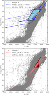 |
Fig. 1 Kiel diagram of the selected samples A and C of bright giant stars. Upper panel: selection of sample A targets (blue dots) in the Kiel diagram using the selection criteria of the calcium query (cf. Appendix A). The box with solid lines shows the initial sample A before we applied the cut-off in Teff. As a visual reference, the grey points represent the MW population from the initial selection (including all stellar types from the GSP-Spec catalogue). We overplot isochrones based on BaSTI stellar evolution models and density contours of the stellar distribution with contour lines enclosing fractions of 90, 75, 60, 45, 30 and 20% of the total number of stars. Lower panel: same, but showing the sample C selection (red dots). The box with dashed lines shows the initial sample C before we applied the cut in Teff. |
3 Abundance maps for young and old disc populations
3.1 Calcium maps
The left panel of Fig. 2 presents the map of the mean calcium abundance with respect to iron ⟨[Ca/Fe]⟩ in the Galactic plane using a smoothing Gaussian bivariate kernel5 with a local bandwidth, h, of 240 pc (cf. Appendix C of Paper I for details about the Gaussian bivariate kernel). For comparison, we also overplot the segments of the nearest spiral arms as traced by the density distribution of upper main-sequence6 (UMS) stars as the solid black lines Poggio et al. (2021). The solid contours show from left to right the Perseus arm, the Local arm, and the Sagittarius-Carina (Sag-Car) arm. As expected, a [Ca/Fe] radial gradient that is more Ca-poor towards the inner parts of the disc is visible, in agreement with the literature (Yong et al. 2006; Lemasle et al. 2013; da Silva et al. 2023). In addition, we detect for the first time the strong azimuthal fluctuations traced by the [Ca/Fe] abundance.
The right panel of Fig. 2 shows the same results for sample C with h=200 pc. The solid black lines show the overdensity contours of the disc giant star population7 studied by Palicio et al. (2023), and show also from left to right the Perseus arm, the Local arm, and the Sag-Car arm. Although the Palicio et al. (2023) selection is based on photometric considerations and might be partially contaminated by young stars, their kinematical analysis (cf. Appendix C of Palicio et al. 2023) suggests that old disc stars dominate the dataset. It is worthwhile mentioning that an older age margin (>3 Gyr) in the Kiel diagram selection for sample C (further reducing the possible contamination from younger stars) has no visible impact on the abundance maps. In addition, a [Ca/Fe] radial gradient that is more Ca-poor towards the inner parts of the disc is again visible. Moreover, we detected azimuthal fluctuations traced by the [Ca/Fe] abundance for the first time, even though they are less evident. The two maps illustrate that a simple radial [Ca/Fe] abundance gradient is not enough to explain the observed abundance distribution. Abundance inhomogeneities appear at different radii and for different azimuths.
To improve the mapping of the Ca abundance inhomogeneities, we defined the [Ca/Fe] excess as [Ca/Fe]loc − [Ca/Fe]large, where [Ca/Fe]loc and [Ca/Fe]large represent the mean [Ca/Fe] smoothed on a local or large scale, respectively. The large scale corresponds to a bandwidth that is six times larger the local one (i.e. hlarge = 1440 pc for sample A and hlarge = 1200 pc for sample C). The resulting map of the [Ca/Fe] excess is presented in the left and right panels of Fig. 3 for sample A and sample C, respectively. In the left panel, the [Ca/Fe] abundance does not increase monotonically as a function of galactocentric radii R (from right to left). It presents local decreases in [Ca/Fe] which corresponds to the lower abundances of [Ca/Fe] in the Local and Sag-Car arms compared to the interarm regions. The obtained [Ca/Fe] patterns can be compared to the [M/H] ones presented in left panel of Fig. 4 (or cf. Paper I for comparison), which showed that stars inside the spiral arms tend to be more metal-rich than those in the inter-arm regions. The anti-correlation between the [M/H] and [Ca/Fe] distributions is characterised by a Spearman coefficient (Spearman 1904) of −0.63, corresponding to a strong anticorrelation (Dancey & Reidy 2007). It is important to note that [M/H] and [Ca/Fe] were derived separately by the GSP-Spec module using different reference grids and methods. Radial and azimuthal fluctuations are clear, but the magnitude of the observed abundance fluctuations is not constant along a given spiral arm. The Perseus arm and the lower part of the Local arm show no [Ca/Fe] deficiency, and the region around (X, Y) = (0, −1) kpc in contrast shows a negative [Ca/Fe] variation that does not correspond to the UMS overdensity contours. The right panel presents the excess map of sample C. It is interesting to point out the sharp correspondence between Palicio et al. (2023) old disc overdensity contours and our observed features. Again, a [Ca/Fe] deficiency in the Sag-Car arm and for the Local arm area is highlighted. To quantify the correlation between the [M/H] and [Ca/Fe] distributions, we estimated the Spearman coefficient. Compared to sample A, the coefficient is equal to −0.68, which again corresponds to a strong negative correlation. For the young sample A, the [Ca/Fe] maps do not clearly match the stellar density distribution for the entire Perseus arm or for the Local arm at negative azimuths.
It is also possible to separately analyse the calcium and iron abundances (i.e. the metallicity). For this purpose, the [Ca/Fe] and [M/H] abundances were combined to obtain the [Ca/H]8 excess map presented in Fig. 5. In our datasets, the [M/H] and [Ca/H] median uncertainties are typically twice smaller than the typical global dispersion of the sample (cf. Table A.1 for the statistical properties of our samples for different chemical abundances). For the young and old populations, the maps of Fig. 5 allow us to directly trace the chemical evolution of calcium separately from iron. Similarly to metallicity (cf. Fig. 4), the calcium abundances show positive fluctuations for the Sagittarius-Carina (Sag-Car) arm and the upper part (Y > −1 kpc, I and II Galactic quadrants) of the Local arm, which reinforces the view that the chemical evolution is faster in the arms than in the interarm regions. The similarity between the [M/H] and [Ca/H] maps is characterised by a Spearman coefficient equal to 0.96 for samples A and C, corresponding to a very strong positive correlation. Again the radial and azimuthal fluctuations are evident, and we note that the magnitude of the observed abundance fluctuations is varies in a given spiral arm. In the Local arm, similarly to [Ca/Fe] excess maps for both samples, regions at Y < 0 are significantly more [Ca/H]-poor or [M/H]-poor than those at Y > 0. The spiral arm signatures for the Perseus arm are only obtained for the [Ca/H] or [M/H] at positive azimuths (larger than 10° in the Cassiopeia region) and only for sample A. Again, we retrieved the region around (X, Y) = (0, −1) kpc only for the young population disc. This time, it shows positive [Ca/H] and [M/H] fluctuations that do not correspond to the UMS overdensity contours. In Sect. 4 we discuss plausible explanations that were proposed for understanding the differences between the density contours and the fluctuations, and the variation in the abundances within the spiral arms in a given arm.
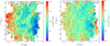 |
Fig. 2 [Ca/Fe] chemical inhomogeneities in the Galactic disc for samples A and C. Left panel: map of [Ca/Fe] abundances for sample A. The black contours indicate the position of the spiral arms obtained using upper main sequence stars from Poggio et al. (2022) that trace from left to right the Perseus arm, the Local arm, and the Sagittarius-Carina arm. The position of the Sun is shown by the black cross at the centre. The Galactic centre is to the right and the Galactic rotation is clockwise. Rings of a constant Galactocentric radius are overplotted as solid grey lines. Right panel: same as the left panel, but for sample C and using the position of the spiral arms found in the subsample of giant stars in Palicio et al. (2023) as black contours. A weak signature of the Gaia scanning law mentioned in the selection function (cf. Appendix A) is still visible, particularly around X ~ 0 kpc and Y = (−4.5, −1) kpc or Y = (2, 4.5) kpc. |
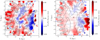 |
Fig. 3 Same as Fig. 2, but now showing the maps of [Ca/Fe] excess and with lines at different azimuthal angles overplotted in grey. Left panel: mean [Ca/Fe] excess in heliocentric coordinates for sample A. Right panel: mean [Ca/Fe] excess in heliocentric coordinates for sample C. |
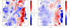 |
Fig. 4 [M/H] chemical inhomogeneities in the Galactic disc for samples A and C. Left panel: map of [M/H] excess for sample A, including the spiral arm contours from Poggio et al. (2021) and adopting a hlocal = 200 pc and a longer scale length, h, that is six times higher. Right panel: same for sample C, including the spiral arm contours from Palicio et al. (2023) and adopting hlocal = 200 pc and hlarge = 1200 pc (i.e. six times higher). |
3.2 Quantification of the observed abundance variations
To better characterise the observed inhomogeneities in the two samples, we show the radial gradients in the [Ca/Fe] abundances in Fig. 6. The left panel of Fig. 6 shows the [Ca/Fe] radial gradient for sample A, which we computed by using a running mean of 5° bin width in azimuth (based on the lines of different azimuthal angles in grey from Fig. 3). As previously mentioned, in addition to the general increase in [Ca/Fe] with Galactic radii, the radial gradients oscillate in correspondence to the azimuthal fluctuations. These radial variations appear to be correlated with the spiral arms in some regions, as discussed above.
For sample C, the radial [Ca/Fe] gradients (cf. right panels of Fig. 6) show significant fluctuations for R<6 kpc that should be considered with caution. Although they might be border effects, it is important to note that these fluctuations are observed consistently in both metallicity and calcium: This is an enrichment of the interstellar medium similar to that expected outside the spiral arms (i.e. an increase in [Ca/Fe] or a depletion in [M/H]). Nevertheless, the observed abundances are also consistent with a chemical bias due to the loss of more metal-rich and [Ca/Fe]-poor stars in the Galactic plane caused by the higher interstellar extinction in these internal regions. Compared to sample A, the slopes observed in sample C highlight smoother radial trends in all azimuthal directions. The [Ca/Fe] gradients vary gradually with ϕ and become slightly steeper for ϕ > 0° (cf. Table 1). They are therefore anticorrelated with the [M/H] gradients reported in Paper I for sample C. However, some fluctuations due to azimuthal changes in the abundance ratios are still visible, but they are flatter than those observed for the young population.
To better visualise the abundances fluctuations in the arm versus inter-arm regions, we selected the stars located inside or outside the spiral arms overdensity in boxes in order to construct an azimuth-averaged radial distribution of each sample. Using the excess data, we computed the median excess variation of all stars within each azimuthal bin across the radial distribution. Fig. 7 shows the variation in the abundance excess as a function of galactocentric radii for different regions in the Galactic disc. Positions in the X − Y plane were assigned to a specific arm segment or to an inter-arm region based on the density distribution of stars. The first inter-arm corresponds to the area between the Local and Sag-Car arms, and the second inter-arm corresponds to the area between the Perseus and Local arms. This way of visualisation indicates that not all the regions in the spiral arms exhibit the same chemical behaviour.
We retrieved broadly similar trends and variations of the chemical abundances for samples A and C. For the first panels with the [Ca/Fe] excess, the inter-arm regions are generally richer in [Ca/Fe] than the arm regions, with the exception of the Perseus arm. In the [Ca/H] case, the chemical pattern in the selected structures is almost the same, which confirms the strong positive correlation found in Sect. 3.1. For a given arm, the [Ca/Fe] excess typically declines as a function of R (and increases for [Ca/H]).
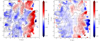 |
Fig. 5 [C/H] chemical inhomogeneities in the Galactic disc for samples A and C. Left panel: map of [Ca/H] excess for sample A, including the spiral arm contours from Poggio et al. (2021) adopting the same local bandwidth as for [Ca/Fe]. Right panel: same for sample C, including the spiral arm contours from Palicio et al. (2023) adopting the same local bandwidth as for [Ca/Fe]. |
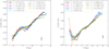 |
Fig. 6 Impact of the observed [Ca/Fe] chemical inhomogeneities on the Galactic gradients. Left panel: radial gradients in the [Ca/Fe] abundances of sample A. The colour code illustrates the results of the running mean applied on the stars contained in the different bins of 5°. Each dot corresponds to the mean of all stars every 1.1 kpc for a specific bin of 5°. Right panel: same as the left panel for sample C. |
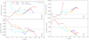 |
Fig. 7 Impact of the observed chemical inhomogeneities on the Galactic gradients. Left panels: azimuth-averaged radial distribution for sample A in bins of 650 pc and excluding those with fewer than 20 stars. From top to bottom, we represent the excess of [Ca/Fe] and [Ca/H] in an azimuth-averaged radial distribution based on the currently known locations of the Galactic disc arms and inter-arm from the density distribution of the stars of the sample. Right panels: same as the left panels, but now for sample C, using bins of 350 pc in galactocentric radius R. Bins with fewer than 200 stars were excluded. |
3.3 Magnesium maps for the youngest sample alone
The [Ca/Fe] abundance maps can be compared to those of [Mg/Fe] in a reduced area (up to distances of about 1.2 kpc around the Sun) because of the imposed threshold in the signal-to-noise (S/N; cf. Appendix A for more details). Thus, sample A includes only 689 stars with [Mg/Fe] abundances that are characterised by a median G magnitude of 7.9 mag (7.1 mag and 8.3 mag are the first and third quartiles of the distribution, respectively). As for the case of [Ca/Fe], we computed the [Mg/Fe] excess to better map the abundances inhomogeneities from the difference [Mg/Fe]loc - [Mg/Fe]large. Because the spatial coverage is shorter, the large-scale length for [Mg/Fe]large was 720 pc (i.e. three times longer than the length we used for the local values [Mg/Fe]loc, i.e. h = 240 pc). Figure 8 illustrates the resulting map of the [Mg/Fe] excess. Despite the reduced area (and the accordingly stronger border effects), the patterns are similar to those in [Ca/Fe] for the Local arm region and its surroundings: The stars within the Local arm tend to be deficient in [Mg/Fe] and [Ca/Fe] with respect to those in the inter-arm regions. At these distances, our sample has not enough stars to quantify the [Mg/Fe] fluctuations in the entire disc, but larger and deeper surveys such as Gaia DR4 will allow us to study them as well as those of many other α-elements.
4 Discussion and conclusions
We have produced 2D chemical abundance maps in the Galactic disc for two α-elements, calcium and magnesium. These maps, based on the [Ca/Fe] and [Mg/Fe] abundances derived by Gaia GSP-Spec, show evidence of considerable radial and azimuthal inhomogeneities, which are accompanied by metallicity fluctuations. Our understanding of the chemical trends in the disc changes from a simplistic 1D radial view to a more complete 2 D perspective that combines radial trends, azimuthal tendencies, and small-scale variations.
For young stellar populations, the inhomogeneities in α-abundances are spatially coherent with the density contours of the Sagittarius-Carina arm and with the Local arm in the first and second Galactic quadrants (Poggio et al. 2021), as already noted for the metallicity signatures in Paper I or in Fig. 4 of this article. In these regions, the global emerging picture is that the stars within the spiral arms are globally (i) more metal-rich (up to ~0–0.20 dex; cf. also Paper I for comparison) and [Ca/H]-rich (~0.18 dex), (ii) more [Ca/Fe]-poor (~0.06 dex) and [Mg/Fe]-poor (~0.05 dex) than the stars in the inter-arm regions, and iii) the magnitude of the observed fluctuations varies in a given spiral arm.
Spiral arms are known possible drivers of chemical azimuthal variations, but their exact influence on the MW disc is still unclear. This is in part due to our lack of knowledge of their dynamical nature (Dobbs & Baba 2014). Lin & Shu (1964) described the spiral patterns in disc galaxies in terms of quasi-stationary density waves that move with a single pattern speed (cf. Shu 2016, for a more recent review). Following this framework, several works tried to estimate the pattern speed of the spiral arms in the MW and obtained values that ranged from ~20 to 40 km/s/kpc (cf. Gerhard 2011, and references therein). Using open clusters (OCs) in Gaia DR 2, Dias et al. (2019) obtained a common pattern speed for the Perseus, Local, and Sagittarius spiral arms of 28.2 ± 2.1 km/s/kpc. This resulted in a co-rotation radius RC = 8.51 ± 0.64 kpc that is not far from the position of the Sun. This is in contrast to the results obtained by Castro-Ginard et al. (2021) based on OCs in Gaia Early Data Release 3, who found that the spiral arms rotate at nearly the same speed as field stars at any given radius. These results discarded a common spiral pattern speed and support the idea of transient spiral arms (Toomre 1964; Sellwood 2012; Hunt et al. 2018).
In the literature, several works modelled spiral arms as a superposition of multiple spiral density waves with different pattern speeds (Tagger et al. 1987; Minchev et al. 2012). Following Minchev et al. (2016), Spitoni et al. (2023) modelled the spiral structure of our Galaxy as a combination of three different segments of varying pattern speeds and developed a 2D chemical evolution model to test their impact on the distribution of chemical elements in the Galactic disc. In their model, the star formation is enhanced by the passage of the spiral arms, and abundance fluctuations are therefore produced with an amplitude depending on the considered chemical species. In the Spitoni et al. (2023) model, elements synthesised on short timescales (i.e. from short-lifetime progenitors) exhibit larger abundance variations as they promptly report the effects of the spiral arm passage, in contrast to other elements that are ejected into the interstellar medium (ISM) after a significant delay. Our analysis globally confirms the predicted Ca enhancement, but with important azimuthal variations. Ca is mainly produced by short-lifetime progenitors (Type II supernovae (SN)), although long-lived progenitors (Type Ia SN) contribute significantly indicated by Kobayashi et al. (2020) or Johnson et al. (2020), the synthesised fraction of Ca produced by Type Ia SN is around 45%.
An important parameter in this picture, as shown by Spitoni et al. (2023), is the time for which a given region of the disc is affected by the spiral arm perturbations. This depends on the total lifetime of the spiral arms, but also on their pattern speed (Spitoni et al. 2023; Debattista et al. 2024). The duration of the spiral arm influence on a particular region of the disc also affects the different abundance ratios and depends on the lifetime of the producers.
Our [Ca/Fe] maps show a tendency to be [Ca/Fe]-poor within the nearest spiral arms. This indicates a higher abundance enhancement of Fe with respect to Ca. This suggests a more complex picture than predicted, as Fe receives a larter contribution from long-lived progenitors (Type Ia SN) than Ca and needs more time than α-elements to dominate the chemical patterns. Consequently, in this context, the [Ca/Fe] depletion of the spiral arms with respect to the inter-arm regions could result from a pattern speed that is close to or fluctuates around the disc corotation for a duration that is compatible with the predominance of the Type Ia SN contribution to the spiral arm chemical pattern (i.e. the duration of the co-rotation with the disc may be longer than previously thought).
To test this hypothesis, we ran new simulations with the 2D chemical evolution model of Spitoni et al. (2023). Figure 9 shows the azimuthal variations in the [Ca/H], [Fe/H] and [Ca/Fe] abundances assuming a spiral arm co-rotation at all radii for 1,3, and 5 Gyr in the upper, middle, and bottom panels, respectively. Similarly to our observations (cf. the left panel of Fig. 2), only the models with a co-rotation of 3 and 5 Gyr start to recover a deficiency in [Ca/Fe] that corresponds to the excess peaks in the [Ca/H] and [Fe/H] variations (around 80 and 260°).
This long co-rotation time between the spiral arms and the disc seems challenging from a dynamical point of view, although it was discussed by several authors in the literature. Sellwood & Carlberg (2014) presented evidence that a long recurrent spiral activity in disc galaxies can result from the superposition of a few transient spiral modes (cf. their Fig. 6). In their simulations, each mode lasted between five and ten rotations at its co-rotation radius, where its amplitude is the greatest. Following Minchev et al. (2016), Spitoni et al. (2023) modelled the spiral structure as formed by the overlap of three chunks with different pattern speeds and spatial extents. Specifically, Spitoni et al. (2023) considered three chunks with pattern speeds of 15,20, and 30 km/s/kpc. In this context, 10 Galactic rotations would correspond to ~4 Gyr, 3 Gyr, and 2 Gyr, respectively. This is coherent with the time needed to explain our observed [Ca/Fe] maps. From the point of view of collisionless N-body simulations (Saha & Elmegreen 2016), the spiral structures of their simulated disc galaxies have given rise to strong long-lasting two-arm spiral wave modes that persisted for about 5 Gyr with a constant pattern speed.
However, several authors, for example Baba et al. (2009) or Quillen et al. (2011), pointed to the fact that a long corotation between the spiral arms and the disc could be very unstable. They suggested that spiral arms are not long-lived features, but rather recurrent phenomena. Interestingly, Grand et al. (2012), whose simulations are not consistent with long-lived spiral arms, suggested that in barred spiral galaxies, the central bar might help to maintain the spiral features for longer (Donner & Thomasson 1994; Binney & Tremaine 2008).
Finally, Khoperskov et al. (2023) studied the impact of the local enrichment and pre-existing radial metallicity gradient transformation on the formation of azimuthal metallicity variations in the vicinity of the spiral arms. Their hydrodynamical simulations suggested that even in the case of co-rotating spirals, the ISM enrichment near the arms alone does probably not cause an azimuthal metallicity pattern, while the key ingredient is a pre-existing radial abundance gradient.
On the other hand, it is interesting to point out that the analysis of the [Ca/Fe] abundance maps for our sample C, whose age is estimated to be older than 2 Gyr, also presents clear [Ca/Fe] deficiencies in the area of the Sag-Car arm and for the Local arm area at positive azimuths. The [Ca/Fe] features correlate with sample C metallicity maps from Paper I (our right panel of Fig. 4) and the azimuthal metallicity variations in RGB stars discussed in Gaia Collaboration (2023b). In addition, the stellar overdensity features that were observed by Palicio et al. (2023) in a much larger sample of giant stars (dominated by old stars) with Gaia full kinematics match the chemical maps of our sample C significantly well and correlate with some parts of the spiral arm loci of young populations.
To minimise the possible presence of young stars in sample C as much as possible, we performed additional tests, such as modifying the age margin in the Kiel diagram (i.e. shifting the left side of the selected area so that it coincides with older isochrones, i.e. 3, 5, or 10 Gyr), or applying a cut in Galactic azimuthal velocity (i.e. removing stars with 210 < Vϕ < 250 km/s). We always obtained maps that were consistent with those presented in Sect. 3 (with an even more marked [Ca/Fe] deficiency in the Local arm for negative azimuths.)
Although we expect to have a small fraction of young star contaminants in our sample C, we cannot completely exclude their presence. We also noted that the Teff > 4200 K cut removes an important fraction of old (cool) stars. It is therefore possible that the (small) fraction of young contaminants partially contributes to the observed azimuthal variations. This makes the interpretation of the maps of sample C more challenging.
Figure 10 presents a pixel-to-pixel diagram of the [Ca/Fe] (upper panel) and [Ca/H] (lower panel) excess based on a comparison of samples A and C. The regions that are most deficient or richest in [Ca/Fe] (and the same holds for [Ca/H]) in our young sample behave in the same way in the older sample, which is characterised by a Spearman coefficient equal to 0.63 (0.67) and which corresponds to a strong positive correlation.
However, it is important to recall that neither the [Ca/Fe] maps of the young population (sample A) nor those of the old one (sample C) present a perfect correlation with the spiral arm loci at all azimuths. The observed [Ca/Fe] deficiencies (or [Ca/H] enhancements) are stronger for the Sag-Car and Local arm at positive azimuths in the direction of the Galactic rotation (for the Local and Perseus arm at positive azimuths and for Sag-Car in the case of [Ca/H]). Similar azimuthal variations in the star formation rate have been observed by Herschel (Elia et al. 2022), which suggests that the chemical maps are linked with a star formation rate that is higher for positive azimuths. Similarly, Widmark & Naik (2024) reported evidence of a spiral arm in the form of an overdensity in the dynamically measured disc surface density. Interestingly, our [Ca/Fe] azimuthal variations are very similar to their residual fluctuations in the vertical gravitational potential that traces the mass overdensity of the spiral arms. Furthermore, Hackshaw et al. (2024) recently explored chemical gradients and azimuthal substructure in the MW disc with giant stars based on data from the Apache Point Observatory Galactic Evolution Experiment (APOGEE) DR 17. They reported azimuthal variations at the level of ±0.05 dex in the Galactic disc. On the other hand, the observed chemical signatures correlate significantly with several known dust structures, such as the Vela molecular ridge (Hottier et al. 2020, 2021) at approximately (X, Y) = (0, −1) kpc (cf. also Paper I), but more weakly with the spiral arm overdensity contours. The dust distribution in the disc is inhomogeneous in the spiral arm structure (Lallement et al. 2022; Vergely et al. 2022), and this plays a role in the chemical evolution through the so-called dust cycle (Spitoni et al. 2017). A detailed study of the correlation between the [M/H] and [Ca/Fe] maps and the corresponding dust distribution will be presented in a future work (Barbillon et al., in prep.).
It is also important to note that spiral arms are not the only potential drivers of chemical azimuthal variations in Galactic discs. For instance, the bar (Di Matteo et al. 2013; Filion et al. 2023) and radial migration induced by satellites (Carr et al. 2022) can also play an important role. This might be particularly important for older stars, which are dynamically relaxed and had time to experience radial stellar migration. On the other hand, young stars are expected to reflect the motion of the gas from which they were recently born.
Finally, we considered the orbital eccentricities of the sample A stars. Although the stars in this young population are globally on quite circular orbits, the eccentricity distribution obtained through the disc showed clear azimuthal variations, with a noticeable correlation with the [Ca/Fe] distribution in the Local arm. Nevertheless, the obtained features are dependent on the considered gravitational potential, and a deeper study needs to be performed with a larger sample of young stars that are less strongly affected by kinematical biases (Poggio et al. 2024). Furthermore, future studies will consider idealised galaxies simulations (Tepper-Garcia et al. 2024) to explore the complex physical processes that govern the current evolution of our Galaxy in more detail. The aim will then be to combine our observational data and simulations to better understand and constrain the structure and evolution of the Galactic disc.
In conclusion, our analysis presented the detection of chemical azimuthal variations in the Galactic disc using α-elements in Gaia GSP-Spec data. It revealed a statistically significant correlation between observed chemical inhomogeneities and the position of the Sagittarius-Carina arm, as well as the Local arm in the first and second Galactic quadrants. Our results open new lines of research into the evolutionary processes of the Galactic disc and its interaction with the spiral arms.
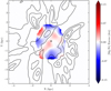 |
Fig. 8 [Mg/Fe] excess map for sample A. The spiral arm contours from Poggio et al. (2021) are overplotted. The local bandwidth is unchanged. |
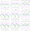 |
Fig. 9 Predicted present-day azimuthal variations in the [Ca/H] (first column), [Fe/H] (second column), and [Ca/Fe] (last column) ratios, computed at different galactocentric distances with the 2D chemical evolution model by Spitoni et al. (2023) with multiple spiral structures. We assumed that for the last 1 Gyr (first row, models A+C3 in Spitoni et al. 2023), 3 Gyr (second row), and 5 Gyr (third row), the co-rotation is extended at all distances. The solid coloured lines indicate the variations at co-rotation loci for the three spiral structures that are characterised by the different pattern speeds indicated in Fig. 1 of Spitoni et al. (2023) before they are extended to all radii. |
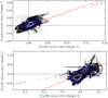 |
Fig. 10 Correlations in the [Ca/Fe] and [Ca/H] excess distributions of the Galactic disc for samples A and C. Upper panel: pixel-to-pixel (black dots) diagram showing the [Ca/Fe] excess variation in sample C as a function of sample A. The blue contours show the distribution of the [Ca/Fe] excess of sample C vs. that of sample A and encloses fractions of 90, 75, 60, 45, 30, and 20% of the total number of pixels. The red line shows a linear fit to the black dots. Bottom panel: same as the upper panel for the [Ca/H] excess case. |
Acknowledgements
MB thanks the anonymous referee for the useful comments that helped improve the quality of the manuscript. This work presents results from the European Space Agency (ESA) space mission Gaia (https://www.cosmos.esa.int/gaia). Gaia data are processed by the Gaia Data Processing and Analysis Consortium (DPAC). Funding for the DPAC is provided by national institutions, in particular the institutions participating in the Gaia MultiLateral Agreement (MLA). The Gaia archive website is (https://archives.esac.esa.int/gaia). MB and PAP acknowledge financial supports from the French Space Agency, Centre National d’Études Spatiales (CNES). ARB, PdL and ES acknowledge funding from the European Union’s Horizon 2020 research and innovation program under SPACE-H2020 grant agreement number 101004214 (EXPLORE project). This project has received funding from the European Union’s Horizon 2020 research and innovation programme under the Marie Sklodowska-Curie grant agreement No. 101063193. We would like to thank the Conseil régional Provence-Alpes-Côte d’Azur for its financial support.
Appendix A Selection criteria
To obtain the initial Gaia dataset for the present analysis, we optimised the procedure described in Appendix A of Paper I to select precise GSP-Spec α-elements abundance estimates. To this purpose, we imposed a limit of 0.1 dex in the [α/Fe] abundance uncertainty and we reduced from 0.50 dex to 0.25 dex the maximum allowed uncertainty in [M/H]. Moreover, the two individual abundance flags (CaUpLim and CaUncer for [Ca/Fe] and MgUpLim and MgUncer for [Mg/Fe] (from Table 2 in Recio-Blanco et al. 2023) are requested to be lower than 2. As a consequence, the definition of the initial working sample is as follows :
[M/H]_unc < 0. 25 & [α/Fe] _unc < 0.1 & vbroadM < 2
& vradM < 2 & fluxNoise < 4 & extrapol < 3
& XUpLim < 2 & XUncer < 2 & KMtypestars < 1
& (astrometric_params_solved = 31
OR astrometric_params_solved = 95) & ruwe < 1.4
& duplicated_source = false
To obtain the Gaia chemo-physical parameters and the kinematics of the selected stars from the Gaia archive, the following query can be submitted (the orange and light blue texts correspond to the calcium and the magnesium specific queries, respectively, and have to be added separately only for studying either the Ca or the Mg):
SELECT g.*, ap.teff_gspspec, ap.teff_gspspec_upper,
ap.teff_gspspec_lower, ap.logg_gspspec, ap.logg_gspspec_upper,
ap.logg_gspspec_lower, ap.mh_gspspec, ap.mh_gspspec_upper,
ap.mh_gspspec_lower, ap.cafe_gspspec, ap.cafe_gspspec_upper
ap.cafe_gspspec_lower, ap.mgfe_gspspec, ap.mgfe_gspspec_upper
ap.mgfe_gspspec_lower, d.r_med_geo, d.r_lo_geo,
d.r_hi_geo, c.vz_med, c.vz_lo, c.vz_hi, c.vphi_med, c.vphi_lo,
c.vphi_hi, c.vrplane_med, c.vrplane_lo, c.vrplane_hi
FROM gaiadr3.gaia_source AS g INNER JOIN
gaiadr3.astrophysical_parameters AS ap ON g.source_id = ap.source_id
INNER JOIN external.gaiaedr3_distance AS d ON
g.source_id = d.source_id INNER JOIN gaiadr3.chemical_cartography
AS c ON g.source_id = c.source_id
WHERE (((mh_gspspec_upper-mh_gspspec_lower)*0.5 < 0.25)
AND ((alphafe_gspspec_upper-alphafe_gspspec_lower)*0.5 < 0.1)
AND ((flags_gspspec LIKE ’__0%’) OR (flags_gspspec LIKE ’__1%’))
AND ((flags_gspspec LIKE ’_____0%’) OR (flags_gspspec LIKE ’_____1%’))
AND ((flags_gspspec LIKE ’______0%’) OR (flags_gspspec LIKE ’______1%’)
OR (flags_gspspec LIKE ’______2%’) OR (flags_gspspec LIKE ’______3%’))
AND ((flags_gspspec LIKE ’_______0%’)
OR (flags_gspspec LIKE ’_______1%’)
OR (flags_gspspec LIKE ’_______2%’))
AND ((flags_gspspec LIKE ’____________0%’)
OR (flags_gspspec LIKE ’____________0%’))
AND ((flags_gspspec LIKE ’_____________________0%’)
OR (flags_gspspec LIKE ’_____________________1%’))
AND ((flags_gspspec LIKE ’______________________0%’)
OR (flags_gspspec LIKE ’______________________1%’)))
AND ((flags_gspspec LIKE ’_______________0%’)
OR (flags_gspspec LIKE ’_______________1%’))
AND ((flags_gspspec LIKE ’________________0%’)
OR (flags_gspspec LIKE ’________________1%’)))
AND (g.astrometric_params_solved = 31
OR g.astrometric_params_solved = 95)
AND g.ruwe < 1.4 AND g.duplicated_source = ’False’
The RVS spectra analysed by GSP-Spec during DR3 operations were selected to have a S/N > 20 before resampling (Recio-Blanco et al. 2023). In this study, we imposed to select stars that have only a S/N > 30 using rv_expected_sig_to_noise from the gaiadr3.astrophysical_parameters table.
For the case of the [Mg/Fe] abundances derived by GSP-Spec from a weak Mg spectral line, we have imposed a threshold in the RVS S/N, selecting stars with rv_expected_sig_to_noise > 250. This avoids biases in the abundance distribution towards the higher, easier to measure abundance values (cf. Contursi et al. 2023, for a similar case that concerns the GSP-Spec [Ce/Fe] abundance). This S/N limit allows to have a median uncertainty in [Mg/Fe] that is almost twice smaller than the dispersion in the observed [Mg/Fe] abundances distribution. The final characteristics of the selected stars in samples A and C, taking into account of all the above described criteria, are summarised in Table A.1.
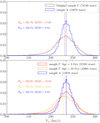 |
Fig. A.1 Distribution of Galactic azimuthal velocities Vϕ for samples A and C. Upper panel: Probability distribution function of Vϕ for sample A and original sample C of this study, normalised to set the area equal to 1. The dark red bars show the stars distribution of sample C, while blue bars show sample A, displayed with median values (P50) and median absolute deviations (MAD) in km/s. Vertical dashed lines denote the median values for each sample. Bottom panel: Same as the upper panel considering sample A and subsets of sample C. The red and orange bars show the stars distribution of sample C for sources below 3 Gyr and over 10 Gyr, respectively, to avoid contribution from stars in each subset. |
Finally, we have explored the spatial distribution of the selected old stars in sample C. To further avoid potential contamination from young stars due to uncertainties in the parameters, we have selected a subsample with Vϕ ≤ 210 km/s. We created the overdensity contours displayed in Fig. A.2. To map these overdensities, we used the procedure described in Poggio et al. (2021), selected a local h=300 pc and larger one hlarger = 1.8 × hlocal pc. It is important to highlight the fact that this analysis has the advantage of selecting a quite pure old population with filtering on chemo-physical and kinematic parameters. However, the drawback is the lower completeness of the sample. Also, as studied by Cantat-Gaudin et al. (2024) (cf. Fig. 9, lower left panel) for a fainter red clump sample, the GSP-Spec completeness diminishes as the distance from the Sun increases, mainly as a function of G magnitude (cf. the right panel of Fig. A.2 for the G magnitude distribution of our sample) and interstellar absorption. Moreover, the completeness can vary significantly depending on the line-of-sight, which probably leads to artefacts when it comes to mapping the distribution of source density in the Galactic plane. A robust study of the density distribution, and therefore, an evaluation of the sample completeness is out of the scope of this paper. Nevertheless, it is interesting to point out that the obtained density maps presented in the left panel of Fig. A.2 reveals a reasonable match with the Palicio et al. (2023) contours. In addition, they show a potential sign of the Perseus Arm in the old population, in agreement with Khanna et al. (2024), who use a very different procedure and a much more complete sample. By removing the Teff cutoff in order to increase the size sample (despite the fact that the scanning law affects particularly a line-of-sight of the studied sample), it is worth noting that the Perseus signature is always visible and a clearer separation between the Local and Sag-Car arms is discernible.
Statistics of sample A and sample C that includes for each element the final number of stars, the limiting Teff, the mean signal-to-noise, the abundances dispersion σ, the median uncertainties, their first and third quartiles distributions.
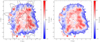 |
Fig. A.2 Correlation between the sample C overdensity and the segments of Palicio et al. (2023) spiral arms in the Galactic disc. Left panel: Overdensity map of sample C with Vϕ ≤ 210 km/s. Here, 13566 stars are considered. The black contours indicate the position of the spiral arms obtained using the sample of giant stars (Palicio et al. 2023). The position of the Sun is indicated by the black cross at (X, Y) = (0, 0) kpc. Right panel: Identical to the left panel, with grey circular outlines that include stars with G ≤ 9, 10, 11, 12 and 13 mag (for the tightest to widest circles). |
References
- Anders, F., Chiappini, C., Minchev, I., et al. 2017, A&A, 600, A70 [NASA ADS] [CrossRef] [EDP Sciences] [Google Scholar]
- Antoja, T., Ramos, P., García-Conde, B., et al. 2023, A&A, 673, A115 [NASA ADS] [CrossRef] [EDP Sciences] [Google Scholar]
- Baba, J., Asaki, Y., Makino, J., et al. 2009, ApJ, 706, 471 [NASA ADS] [CrossRef] [Google Scholar]
- Bailer-Jones, C. A. L., Rybizki, J., Fouesneau, M., Demleitner, M., & Andrae, R. 2021, VizieR Online Data Catalog I/352 [Google Scholar]
- Balser, D. S., Rood, R. T., Bania, T. M., & Anderson, L. D. 2011, ApJ, 738, 27 [NASA ADS] [CrossRef] [Google Scholar]
- Binney, J., & Tremaine, S. 2008, Galactic Dynamics 2nd edn. [Google Scholar]
- Bland-Hawthorn, J., Sharma, S., Tepper-Garcia, T., et al. 2019, MNRAS, 486, 1167 [NASA ADS] [CrossRef] [Google Scholar]
- Cantat-Gaudin, T., Fouesneau, M., Rix, H.-W., et al. 2024, A&A, 683, A128 [NASA ADS] [CrossRef] [EDP Sciences] [Google Scholar]
- Carr, C., Johnston, K. V., Laporte, C. F. P., & Ness, M. K. 2022, MNRAS, 516, 5067 [NASA ADS] [CrossRef] [Google Scholar]
- Castro-Ginard, A., McMillan, P. J., Luri, X., et al. 2021, A&A, 652, A162 [NASA ADS] [CrossRef] [EDP Sciences] [Google Scholar]
- Contursi, G., de Laverny, P., Recio-Blanco, A., et al. 2023, A&A, 670, A106 [NASA ADS] [CrossRef] [EDP Sciences] [Google Scholar]
- Creevey, O. L., Sordo, R., Pailler, F., et al. 2023, A&A, 674, A26 [NASA ADS] [CrossRef] [EDP Sciences] [Google Scholar]
- da Silva, R., D’Orazi, V., Palla, M., et al. 2023, A&A, 678, A195 [NASA ADS] [CrossRef] [EDP Sciences] [Google Scholar]
- Dancey, C., & Reidy, J. 2007, Statistics Without Maths for Psychology, British Psychological Society book [Google Scholar]
- De Cia, A., Jenkins, E. B., Fox, A. J., et al. 2021, Nature, 597, 206 [NASA ADS] [CrossRef] [Google Scholar]
- Debattista, V. P., Khachaturyants, T., Amarante, J. A. S., et al. 2024, arXiv e-prints [arXiv:2402.08356] [Google Scholar]
- Di Matteo, P., Haywood, M., Combes, F., Semelin, B., & Snaith, O. N. 2013, A&A, 553, A102 [NASA ADS] [CrossRef] [EDP Sciences] [Google Scholar]
- Dias, W. S., Monteiro, H., Lépine, J. R. D., & Barros, D. A. 2019, MNRAS, 486, 5726 [NASA ADS] [CrossRef] [Google Scholar]
- Dobbs, C., & Baba, J. 2014, PASA, 31, e035 [NASA ADS] [CrossRef] [Google Scholar]
- Donner, K. J., & Thomasson, M. 1994, A&A, 290, 785 [NASA ADS] [Google Scholar]
- Elia, D., Molinari, S., Schisano, E., et al. 2022, ApJ, 941, 162 [NASA ADS] [CrossRef] [Google Scholar]
- Filion, C., McClure, R. L., Weinberg, M. D., D’Onghia, E., & Daniel, K. J. 2023, MNRAS, 524, 276 [Google Scholar]
- Gaia Collaboration (Drimmel, R., et al.) 2023a, A&A, 674, A37 [CrossRef] [EDP Sciences] [Google Scholar]
- Gaia Collaboration (Recio-Blanco, A., et al.) 2023b, A&A, 674, A38 [CrossRef] [EDP Sciences] [Google Scholar]
- Gaia Collaboration (Vallenari, A., et al.) 2023c, A&A, 674, A1 [NASA ADS] [CrossRef] [EDP Sciences] [Google Scholar]
- Garavito-Camargo, N., Besla, G., Laporte, C. F. P., et al. 2021, ApJ, 919, 109 [NASA ADS] [CrossRef] [Google Scholar]
- Genovali, K., Lemasle, B., Bono, G., et al. 2014, A&A, 566, A37 [NASA ADS] [CrossRef] [EDP Sciences] [Google Scholar]
- Georgelin, Y. M., & Georgelin, Y. P. 1976, A&A, 49, 57 [NASA ADS] [Google Scholar]
- Gerhard, O. 2011, Mem. Soc. Astron. Ital. Suppl., 18, 185 [Google Scholar]
- Gilmore, G., & Reid, N. 1983, MNRAS, 202, 1025 [Google Scholar]
- Grand, R. J. J., Kawata, D., & Cropper, M. 2012, MNRAS, 421, 1529 [CrossRef] [Google Scholar]
- Grand, R. J. J., Springel, V., Kawata, D., et al. 2016, MNRAS, 460, L94 [Google Scholar]
- Hackshaw, Z., Hawkins, K., Filion, C., et al. 2024, arXiv e-prints [arXiv:2405.18120] [Google Scholar]
- Hawkins, K. 2023, MNRAS, 525, 3318 [NASA ADS] [CrossRef] [Google Scholar]
- Helmi, A., Babusiaux, C., Koppelman, H. H., et al. 2018, Nature, 563, 85 [Google Scholar]
- Hidalgo, S. L., Pietrinferni, A., Cassisi, S., et al. 2018, ApJ, 856, 125 [Google Scholar]
- Hottier, C., Babusiaux, C., & Arenou, F. 2020, A&A, 641, A79 [NASA ADS] [CrossRef] [EDP Sciences] [Google Scholar]
- Hottier, C., Babusiaux, C., & Arenou, F. 2021, A&A, 655, A68 [NASA ADS] [CrossRef] [EDP Sciences] [Google Scholar]
- Hunt, J. A. S., Hong, J., Bovy, J., Kawata, D., & Grand, R. J. J. 2018, MNRAS, 481, 3794 [NASA ADS] [CrossRef] [Google Scholar]
- Hunt, J. A. S., Bub, M. W., Bovy, J., et al. 2019, MNRAS, 490, 1026 [NASA ADS] [CrossRef] [Google Scholar]
- Johnson, J. A., Fields, B. D., & Thompson, T. A. 2020, Philos. Trans. Roy. Soc. Lond. Ser. A, 378, 20190301 [Google Scholar]
- Katz, D., Gómez, A., Haywood, M., Snaith, O., & Di Matteo, P. 2021, A&A, 655, A111 [NASA ADS] [CrossRef] [EDP Sciences] [Google Scholar]
- Khanna, S., Yu, J., Drimmel, R., et al. 2024, arXiv e-prints [arXiv:2410.22036] [Google Scholar]
- Khoperskov, S., Di Matteo, P., Haywood, M., & Combes, F. 2018, A&A, 611, L2 [NASA ADS] [CrossRef] [EDP Sciences] [Google Scholar]
- Khoperskov, S., Gerhard, O., Di Matteo, P., et al. 2020, A&A, 634, L8 [NASA ADS] [CrossRef] [EDP Sciences] [Google Scholar]
- Khoperskov, S., Sivkova, E., Saburova, A., et al. 2023, A&A, 671, A56 [NASA ADS] [CrossRef] [EDP Sciences] [Google Scholar]
- Kobayashi, C., Karakas, A. I., & Lugaro, M. 2020, ApJ, 900, 179 [Google Scholar]
- Kovtyukh, V., Lemasle, B., Bono, G., et al. 2022, MNRAS, 510, 1894 [Google Scholar]
- Lallement, R., Vergely, J. L., Babusiaux, C., & Cox, N. L. J. 2022, A&A, 661, A147 [NASA ADS] [CrossRef] [EDP Sciences] [Google Scholar]
- Laporte, C. F. P., Johnston, K. V., Gómez, F. A., Garavito-Camargo, N., & Besla, G. 2018, MNRAS, 481, 286 [Google Scholar]
- Lemasle, B., François, P., Genovali, K., et al. 2013, A&A, 558, A31 [NASA ADS] [CrossRef] [EDP Sciences] [Google Scholar]
- Lin, C. C., & Shu, F. H. 1964, ApJ, 140, 646 [Google Scholar]
- Minchev, I., Famaey, B., Quillen, A. C., et al. 2012, A&A, 548, A126 [NASA ADS] [CrossRef] [EDP Sciences] [Google Scholar]
- Minchev, I., Chiappini, C., & Martig, M. 2016, Astron. Nachr., 337, 944 [CrossRef] [Google Scholar]
- Minniti, J. H., Zoccali, M., Rojas-Arriagada, A., et al. 2021, A&A, 654, A138 [NASA ADS] [CrossRef] [EDP Sciences] [Google Scholar]
- Mollá, M., Wekesa, S., Cavichia, O., et al. 2019, MNRAS, 490, 665 [CrossRef] [Google Scholar]
- Okuda, H., Maihara, T., Oda, N., & Sugiyama, T. 1977, Nature, 265, 515 [NASA ADS] [CrossRef] [Google Scholar]
- Palicio, P. A., Martinez-Valpuesta, I., Allende Prieto, C., et al. 2018, MNRAS, 478, 1231 [NASA ADS] [CrossRef] [Google Scholar]
- Palicio, P., Recio-Blanco, A., Poggio, E., et al. 2023, A&A, 670, L7 [NASA ADS] [CrossRef] [EDP Sciences] [Google Scholar]
- Pilyugin, L. S., Grebel, E. K., & Kniazev, A. Y. 2014, AJ, 147, 131 [NASA ADS] [CrossRef] [Google Scholar]
- Poggio, E., Drimmel, R., Cantat-Gaudin, T., et al. 2021, A&A, 651, A104 [NASA ADS] [CrossRef] [EDP Sciences] [Google Scholar]
- Poggio, E., Recio-Blanco, A., Palicio, P. A., et al. 2022, A&A, 666, L4 [NASA ADS] [CrossRef] [EDP Sciences] [Google Scholar]
- Poggio, E., Khanna, S., Drimmel, R., et al. 2024, arXiv e-prints [arXiv:2407.18659] [Google Scholar]
- Purcell, C. W., Bullock, J. S., Tollerud, E. J., Rocha, M., & Chakrabarti, S. 2011, Nature, 477, 301 [Google Scholar]
- Quillen, A. C., Dougherty, J., Bagley, M. B., Minchev, I., & Comparetta, J. 2011, MNRAS, 417, 762 [NASA ADS] [CrossRef] [Google Scholar]
- Recio-Blanco, A., de Laverny, P., Palicio, P. A., et al. 2023, A&A, 674, A29 [NASA ADS] [CrossRef] [EDP Sciences] [Google Scholar]
- Recio-Blanco, A., de Laverny, P., Palicio, P. A., et al. 2024, arXiv e-prints [arXiv:2402.01522] [Google Scholar]
- Reid, M. J., Menten, K. M., Brunthaler, A., et al. 2019, ApJ, 885, 131 [Google Scholar]
- Saha, K., & Elmegreen, B. 2016, ApJ, 826, L21 [NASA ADS] [CrossRef] [Google Scholar]
- Santos-Peral, P., Recio-Blanco, A., Kordopatis, G., Fernández-Alvar, E., & de Laverny, P. 2021, A&A, 653, A85 [NASA ADS] [CrossRef] [EDP Sciences] [Google Scholar]
- Schönrich, R., & Binney, J. 2009, MNRAS, 396, 203 [Google Scholar]
- Sellwood, J. A. 2012, ApJ, 751, 44 [NASA ADS] [CrossRef] [Google Scholar]
- Sellwood, J. A., & Carlberg, R. G. 2014, ApJ, 785, 137 [CrossRef] [Google Scholar]
- Shu, F. H. 2016, ARA&A, 54, 667 [NASA ADS] [CrossRef] [Google Scholar]
- Spearman, C. 1904, Am. J. Psychol., 15, 72 [Google Scholar]
- Spitoni, E., Gioannini, L., & Matteucci, F. 2017, A&A, 605, A38 [NASA ADS] [CrossRef] [EDP Sciences] [Google Scholar]
- Spitoni, E., Cescutti, G., Minchev, I., et al. 2019, A&A, 628, A38 [NASA ADS] [CrossRef] [EDP Sciences] [Google Scholar]
- Spitoni, E., Cescutti, G., Recio-Blanco, A., et al. 2023, A&A, 680, A85 [NASA ADS] [CrossRef] [EDP Sciences] [Google Scholar]
- Tagger, M., Sygnet, J. F., Athanassoula, E., & Pellat, R. 1987, ApJ, 318, L43 [NASA ADS] [CrossRef] [Google Scholar]
- Taylor, J. H., & Cordes, J. M. 1993, ApJ, 411, 674 [Google Scholar]
- Tepper-Garcia, T., Bland-Hawthorn, J., Vasiliev, E., et al. 2024, arXiv e-prints [arXiv:2406.00342] [Google Scholar]
- Toomre, A. 1964, ApJ, 139, 1217 [Google Scholar]
- Vergely, J. L., Lallement, R., & Cox, N. L. J. 2022, A&A, 664, A174 [NASA ADS] [CrossRef] [EDP Sciences] [Google Scholar]
- Vogt, F. P. A., Pérez, E., Dopita, M. A., Verdes-Montenegro, L., & Borthakur, S. 2017, A&A, 601, A61 [NASA ADS] [CrossRef] [EDP Sciences] [Google Scholar]
- Wenger, T. V., Balser, D. S., Anderson, L. D., & Bania, T. M. 2019, ApJ, 887, 114 [NASA ADS] [CrossRef] [Google Scholar]
- Widmark, A., & Naik, A. P. 2024, A&A, 686, A70 [NASA ADS] [CrossRef] [EDP Sciences] [Google Scholar]
- Yong, D., Carney, B. W., Teixera de Almeida, M. L., & Pohl, B. L. 2006, AJ, 131, 2256 [NASA ADS] [CrossRef] [Google Scholar]
- Zurita, A., Florido, E., Bresolin, F., Pérez-Montero, E., & Pérez, I. 2021, MNRAS, 500, 2359 [Google Scholar]
In the GSP-Spec catalogue, [M/H] traces the iron abundances [Fe/H] as iron lines dominate the non-α-elements feature used by GSP-Spec. The [α/Fe] parameter is dominated by the [Ca/Fe] abundance, since the Ca II triplet absorption dominates the α-elements signatures in the Radial Velocity Spectrometer (RVS) spectral domain.
As discussed in Poggio et al. (2021), the choice of kernel type (e.g. Gaussian, Epanechnikov...) does not have a significant impact on the obtained maps.
Revised selection of more than 600 000 UMS stars from a cross match between photometric measurements from the 2-Micron All Sky Survey (2MASS) and Gaia (cf. Sect. 2.1 of Poggio et al. 2021).
Sample selected from Gaia DR3 using photometry and imposing criteria in order to limit contribution of main sequence and faint dwarf stars (cf. Appendix C of Palicio et al. 2023).
All Tables
Statistics of sample A and sample C that includes for each element the final number of stars, the limiting Teff, the mean signal-to-noise, the abundances dispersion σ, the median uncertainties, their first and third quartiles distributions.
All Figures
|
Fig. 1 Kiel diagram of the selected samples A and C of bright giant stars. Upper panel: selection of sample A targets (blue dots) in the Kiel diagram using the selection criteria of the calcium query (cf. Appendix A). The box with solid lines shows the initial sample A before we applied the cut-off in Teff. As a visual reference, the grey points represent the MW population from the initial selection (including all stellar types from the GSP-Spec catalogue). We overplot isochrones based on BaSTI stellar evolution models and density contours of the stellar distribution with contour lines enclosing fractions of 90, 75, 60, 45, 30 and 20% of the total number of stars. Lower panel: same, but showing the sample C selection (red dots). The box with dashed lines shows the initial sample C before we applied the cut in Teff. |
| In the text | |
|
Fig. 2 [Ca/Fe] chemical inhomogeneities in the Galactic disc for samples A and C. Left panel: map of [Ca/Fe] abundances for sample A. The black contours indicate the position of the spiral arms obtained using upper main sequence stars from Poggio et al. (2022) that trace from left to right the Perseus arm, the Local arm, and the Sagittarius-Carina arm. The position of the Sun is shown by the black cross at the centre. The Galactic centre is to the right and the Galactic rotation is clockwise. Rings of a constant Galactocentric radius are overplotted as solid grey lines. Right panel: same as the left panel, but for sample C and using the position of the spiral arms found in the subsample of giant stars in Palicio et al. (2023) as black contours. A weak signature of the Gaia scanning law mentioned in the selection function (cf. Appendix A) is still visible, particularly around X ~ 0 kpc and Y = (−4.5, −1) kpc or Y = (2, 4.5) kpc. |
| In the text | |
|
Fig. 3 Same as Fig. 2, but now showing the maps of [Ca/Fe] excess and with lines at different azimuthal angles overplotted in grey. Left panel: mean [Ca/Fe] excess in heliocentric coordinates for sample A. Right panel: mean [Ca/Fe] excess in heliocentric coordinates for sample C. |
| In the text | |
|
Fig. 4 [M/H] chemical inhomogeneities in the Galactic disc for samples A and C. Left panel: map of [M/H] excess for sample A, including the spiral arm contours from Poggio et al. (2021) and adopting a hlocal = 200 pc and a longer scale length, h, that is six times higher. Right panel: same for sample C, including the spiral arm contours from Palicio et al. (2023) and adopting hlocal = 200 pc and hlarge = 1200 pc (i.e. six times higher). |
| In the text | |
|
Fig. 5 [C/H] chemical inhomogeneities in the Galactic disc for samples A and C. Left panel: map of [Ca/H] excess for sample A, including the spiral arm contours from Poggio et al. (2021) adopting the same local bandwidth as for [Ca/Fe]. Right panel: same for sample C, including the spiral arm contours from Palicio et al. (2023) adopting the same local bandwidth as for [Ca/Fe]. |
| In the text | |
|
Fig. 6 Impact of the observed [Ca/Fe] chemical inhomogeneities on the Galactic gradients. Left panel: radial gradients in the [Ca/Fe] abundances of sample A. The colour code illustrates the results of the running mean applied on the stars contained in the different bins of 5°. Each dot corresponds to the mean of all stars every 1.1 kpc for a specific bin of 5°. Right panel: same as the left panel for sample C. |
| In the text | |
|
Fig. 7 Impact of the observed chemical inhomogeneities on the Galactic gradients. Left panels: azimuth-averaged radial distribution for sample A in bins of 650 pc and excluding those with fewer than 20 stars. From top to bottom, we represent the excess of [Ca/Fe] and [Ca/H] in an azimuth-averaged radial distribution based on the currently known locations of the Galactic disc arms and inter-arm from the density distribution of the stars of the sample. Right panels: same as the left panels, but now for sample C, using bins of 350 pc in galactocentric radius R. Bins with fewer than 200 stars were excluded. |
| In the text | |
|
Fig. 8 [Mg/Fe] excess map for sample A. The spiral arm contours from Poggio et al. (2021) are overplotted. The local bandwidth is unchanged. |
| In the text | |
|
Fig. 9 Predicted present-day azimuthal variations in the [Ca/H] (first column), [Fe/H] (second column), and [Ca/Fe] (last column) ratios, computed at different galactocentric distances with the 2D chemical evolution model by Spitoni et al. (2023) with multiple spiral structures. We assumed that for the last 1 Gyr (first row, models A+C3 in Spitoni et al. 2023), 3 Gyr (second row), and 5 Gyr (third row), the co-rotation is extended at all distances. The solid coloured lines indicate the variations at co-rotation loci for the three spiral structures that are characterised by the different pattern speeds indicated in Fig. 1 of Spitoni et al. (2023) before they are extended to all radii. |
| In the text | |
|
Fig. 10 Correlations in the [Ca/Fe] and [Ca/H] excess distributions of the Galactic disc for samples A and C. Upper panel: pixel-to-pixel (black dots) diagram showing the [Ca/Fe] excess variation in sample C as a function of sample A. The blue contours show the distribution of the [Ca/Fe] excess of sample C vs. that of sample A and encloses fractions of 90, 75, 60, 45, 30, and 20% of the total number of pixels. The red line shows a linear fit to the black dots. Bottom panel: same as the upper panel for the [Ca/H] excess case. |
| In the text | |
|
Fig. A.1 Distribution of Galactic azimuthal velocities Vϕ for samples A and C. Upper panel: Probability distribution function of Vϕ for sample A and original sample C of this study, normalised to set the area equal to 1. The dark red bars show the stars distribution of sample C, while blue bars show sample A, displayed with median values (P50) and median absolute deviations (MAD) in km/s. Vertical dashed lines denote the median values for each sample. Bottom panel: Same as the upper panel considering sample A and subsets of sample C. The red and orange bars show the stars distribution of sample C for sources below 3 Gyr and over 10 Gyr, respectively, to avoid contribution from stars in each subset. |
| In the text | |
|
Fig. A.2 Correlation between the sample C overdensity and the segments of Palicio et al. (2023) spiral arms in the Galactic disc. Left panel: Overdensity map of sample C with Vϕ ≤ 210 km/s. Here, 13566 stars are considered. The black contours indicate the position of the spiral arms obtained using the sample of giant stars (Palicio et al. 2023). The position of the Sun is indicated by the black cross at (X, Y) = (0, 0) kpc. Right panel: Identical to the left panel, with grey circular outlines that include stars with G ≤ 9, 10, 11, 12 and 13 mag (for the tightest to widest circles). |
| In the text | |
Current usage metrics show cumulative count of Article Views (full-text article views including HTML views, PDF and ePub downloads, according to the available data) and Abstracts Views on Vision4Press platform.
Data correspond to usage on the plateform after 2015. The current usage metrics is available 48-96 hours after online publication and is updated daily on week days.
Initial download of the metrics may take a while.