| Issue |
A&A
Volume 693, January 2025
|
|
|---|---|---|
| Article Number | A278 | |
| Number of page(s) | 23 | |
| Section | Interstellar and circumstellar matter | |
| DOI | https://doi.org/10.1051/0004-6361/202450863 | |
| Published online | 23 January 2025 | |
MINDS. JWST-MIRI reveals a peculiar CO2-rich chemistry in the drift-dominated disk CX Tau
1
Leiden Observatory, Leiden University,
2300 RA
Leiden,
The Netherlands
2
Max-Planck Institut für Extraterrestrische Physik (MPE),
Giessenbachstr. 1,
85748,
Garching,
Germany
3
Department of Astrophysics, University of Vienna,
Türkenschanzstr. 17,
1180
Vienna,
Austria
4
ETH Zürich, Institute for Particle Physics and Astrophysics,
Wolfgang-Pauli-Str. 27,
8093
Zürich,
Switzerland
5
Max-Planck-Institut für Astronomie (MPIA),
Königstuhl 17,
69117
Heidelberg,
Germany
6
Université Paris-Saclay, Université Paris Cité, CEA, CNRS, AIM,
91191
Gif-sur-Yvette,
France
7
Centro de Astrobiología (CAB), CSIC-INTA,
ESAC Campus, Camino Bajo del Castillo s/n,
28692
Villanueva de la Cañada, Madrid,
Spain
8
INAF – Osservatorio Astronomico di Capodimonte,
Salita Moiariello 16,
80131
Napoli,
Italy
9
Dublin Institute for Advanced Studies,
31 Fitzwilliam Place,
D02 XF86
Dublin,
Ireland
10
Kapteyn Astronomical Institute, Rijksuniversiteit Groningen,
Postbus 800,
9700AV
Groningen,
The Netherlands
11
SRON Netherlands Institure for Space Research,
PO Box 800,
9700 AV,
Groningen,
The Netherlands
12
Department of Astronomy, Stockholm University, AlbaNova University Center,
10691
Stockholm,
Sweden
13
Institute of Astronomy, KU Leuven,
Celestijnenlaan 200D,
3001
Leuven,
Belgium
14
STAR Institute, Université de Liège,
Allée du Six Août 19c,
4000
Liège,
Belgium
15
Department of Astrophysics/IMAPP, Radboud University,
PO Box 9010,
6500 GL
Nijmegen,
The Netherlands
16
Université Paris-Saclay, CNRS, Institut d’Astrophysique Spatiale,
91405
Orsay,
France
★ Corresponding author; vlasblom@strw.leidenuniv.nl
Received:
24
May
2024
Accepted:
13
December
2024
Context. Radial drift of icy pebbles can have a large impact on the chemistry of the inner regions of protoplanetary disks, where most terrestrial planets are thought to form. Disks with compact millimeter dust emission (≲50 au) are suggested to have a higher H2O flux than more extended disks, as well as show excess cold H2O emission, likely due to efficient radial drift bringing H2O-rich material to the inner disk, where it can be observed with IR facilities such as the James Webb Space Telescope (JWST).
Aims. We present JWST MIRI/MRS observations of the disk around the low-mass T Tauri star CX Tau (M2.5, 0.37 M⊙) taken as a part of the Mid-INfrared Disk Survey (MINDS) GTO program, a prime example of a drift-dominated disk based on ALMA data. In the context of compact disks, this disk seems peculiar: the source possesses a bright CO2 feature instead of the bright H2O that could perhaps be expected based on the efficient radial drift. We aim to provide an explanation for this finding in the context of the radial drift of ices and the disk’s physical structure.
Methods. We modeled the molecular features in the spectrum using local thermodynamic equilibrium (LTE) 0D slab models, which allowed us to obtain estimates of the temperature, column density, and emitting area of the emission.
Results. We detect molecular emission from H2O, 12CO2, 13CO2, C2H2, HCN, and OH in this disk, and even demonstrate a potential detection of CO 18O emission. Analysis of the 12CO2 and 13CO2 emission shows the former to be optically thick and tracing a temperature of ∼450 K at an (equivalent) emitting radius of ∼0.05 au. The optically thinner isotopologue traces significantly colder temperatures (∼200 K) and a larger emitting area. Both the ro-vibrational bands of H2O at shorter wavelengths and its pure rotational bands at longer wavelengths are securely detected. Both sets of lines are optically thick, tracing a similar temperature of ∼500–600 K and emitting area as the CO2 emission. We also find evidence for an even colder, ∼200 K H2O component at longer wavelengths, which is in line with this disk having strong radial drift. We also find evidence of highly excited rotational OH emission at 9–11 µm, known as “prompt emission”, caused by H2O photodissociation. Additionally, we firmly detect four pure rotational lines of H2, which show evidence of extended emission. Finally, we also detect several H recombination lines and the [Ne II] line.
Conclusions. The cold temperatures found for both the 13CO2 and H2O emission at longer wavelengths indicate that the radial drift of ices likely plays an important role in setting the chemistry of the inner disk of CX Tau. The H2O-rich gas has potentially already advected onto the central star, which is now followed by an enhancement of comparatively CO2-rich gas reaching the inner disk, explaining the enhancement of CO2 emission in CX Tau. The comparatively weaker H2O emission can be explained by the source’s low accretion luminosity. Alternatively, the presence of a small, inner cavity with a size of roughly 2 au in radius, outside the H2O iceline, could explain the bright CO2 emission. Higher angular resolution ALMA observations are needed to test this.
Key words: astrochemistry / protoplanetary disks / stars: variables: T Tauri / Herbig Ae/Be / infrared: general
© The Authors 2025
 Open Access article, published by EDP Sciences, under the terms of the Creative Commons Attribution License (https://creativecommons.org/licenses/by/4.0), which permits unrestricted use, distribution, and reproduction in any medium, provided the original work is properly cited.
This article is published in open access under the Subscribe to Open model. Subscribe to A&A to support open access publication.
1 Introduction
The chemistry of the inner few au of protoplanetary disks is an important factor in setting the atmospheric composition of exoplanets. Most planets are thought to form in this region and thus their bulk elemental inventory is set by that of their parent disk (Dawson & Johnson 2018; Öberg & Bergin 2021). The hot, inner regions of the disk are best characterized in the infrared (IR). This can now be done in greater detail than ever before with the James Webb Space Telescope (JWST) (e.g., Kóspál et al. 2023; Banzatti et al. 2023a; Kamp et al. 2023; van Dishoeck et al. 2023; Henning et al. 2024; Pontoppidan et al. 2024; Romero-Mirza et al. 2024a), with its higher sensitivity and higher spectral resolution even enabling the first detection of 13CO2 in a T Tauri disk (Grant et al. 2023), as well as a large variety of hydrocarbons in disks around very low-mass stars (Tabone et al. 2023; Arabhavi et al. 2024; Kanwar et al. 2024). This shows the capability of JWST to uncover the chemistry of these inner regions in unprecedented detail.
The chemical composition of the disk is linked closely to the disk’s physical structure, especially to the transport (or lack thereof) of dust grains. In the outer disk, these dust grains contain an icy mantle composed of several frozen-out species, such as H2O, CO2, NH3, and CO. When these dust grains drift inward and cross each species’ iceline, the sublimating ice can enrich the gas, changing the elemental composition of the disk with radius, which can be traced by, for example, the C/O ratio (Öberg et al. 2011; Booth et al. 2017). The C/O ratio in the disk changes not only with radius, but also with time. This is demonstrated by Kalyaan et al. (2021, 2023) and Mah et al. (2023, 2024), who show that the delivery of O-rich pebbles from just outside the H2O iceline first leads to a decrease of the C/O ratio in the innermost part of the disk. The subsequent draining of this O-rich gas onto the star, combined with the delivery of more C-rich gas advecting inward from the outer disk, increases this ratio again over time. Krijt et al. (2018, 2020) show a similar effect in their modeling work, where the sequestration of species such as CO in ices can lead to a depletion in the gas-phase abundance higher up in the disk, thus changing the C/O ratio. Kalyaan et al. (2021, 2023) also demonstrate how gaps at different locations in the disks can affect this process, similar to the works by Bitsch & Mah (2023) and Lienert et al. (2024) who investigate the effects of gap-opening on the C/O ratio caused by a giant planet and internal photo-evaporation, respectively. Work by Sellek et al. (2024) also demonstrates how disks can undergo a CO2 -rich phase with time, which is sensitive to the location of a possible gap and seems to be traced well by the CO2 column density.
The Atacama Large Millimeter/sub-millimeter Array (ALMA) shows that many disks have substructures in the dust out to large scales (see, e.g., Andrews et al. 2018; Huang et al. 2018; Long et al. 2018), which could halt this drift and subsequent enrichment of the gas (Kalyaan et al. 2021, 2023). However, this ubiquity of substructures seems to be limited to the brightest and largest disks, as larger surveys seem to instead find most disks to be very compact, with no discernible substructures (Ansdell et al. 2018; Cieza et al. 2019; Long et al. 2019). This could be a result of the initial collapsing cloud core having a low angular momentum, allowing it to form a small, compact disk. However, dust grains are also known to drift radially inward very rapidly, possibly making the dust disk more compact over time.
To distinguish between these two scenarios, a good method is to compare the millimeter dust disk size to the gas disk size as traced by CO emission. After all, the gas is not subject to the same efficient radial drift as the dust, so it is expected to retain its initial size, which would be much larger than the millimeter dust disk. In the case of low initial angular momentum, the gas and dust disks would be expected to have a more similar size. Modeling work shows that radial drift can indeed be the cause of (sufficiently large; Rgas/Rdust≳4) differences between the dust disk extent and the gas disk extent (see Facchini et al. 2017; Trapman et al. 2019, 2020).
One of the most extreme examples of a drift-dominated disk found to date is CX Tau, a disk around an M2.5 star in the Taurus-Auriga star-forming region at a distance of 127.9 ± 0.7 pc (Gaia Collaboration 2018). High-resolution ALMA observations (~40 mas, corresponding to ~5 au at 128 pc) find a 68% dust disk radius of only ~15 au, whereas the 68% gas disk radius in 12CO extends out to ~75 au, yielding Rgas/Rdust ~ 5 (Facchini et al. 2019), a difference that can only be achieved through very efficient radial drift.
Naturally, one would expect that the chemistry of the inner regions differs between a compact disk with efficient radial drift and a large disk with substructures halting this process. This is suggested to be the case by Banzatti et al. (2020), who find a correlation between the H2O flux observed with Spitzer and the dust disk size, with the smaller disks being more H2O-rich. This correlation is also theoretically motivated with modeling work by Kalyaan et al. (2021). The larger H2O flux in compact disks is attributed to the efficient radial drift in compact disks delivering H2O-rich ices to the inner regions. More recent work by Banzatti et al. (2023a) also shows that compact disks show excess cool H2O emission, which can likely be attributed to efficient radial drift as well.
We present observations of CX Tau taken with the MidInfraRed Instrument (MIRI; Rieke et al. 2015; Wright et al. 2015, 2023) Medium Resolution Spectrometer (MRS; Wells et al. 2015; Argyriou et al. 2023) on board JWST, taken as part of the MIRI Mid-INfrared Disk Survey (MINDS) GTO program (PID: 1282, PI: T. Henning; see Henning et al. 2024 for an overview of the program). The central star has a luminosity of L* = 0.22 ± 0.11 L⊙, an effective temperature Teff = 3483 ± 48 K (Herczeg & Hillenbrand 2014), a dynamical estimate of its mass of M* = 0.37 M⊙ (Simon et al. 2017), and a mass accretion rate of Macc = 7.1 × 10⁻¹⁰ M⊙ yr–1 (Hartmann et al. 1998). The source was also observed with Spitzer (Furlan et al. 2006; Najita et al. 2007; Furlan et al. 2011), but its molecular features have not been analyzed before. We detect mid-IR emission from H2O, 12CO2, 13CO2, C2H2, HCN, and OH for the first time in this disk, and even present a potential detection of CO18O. We use local thermodynamic equilibrium (LTE) slab models to constrain the properties of the emission and use the relative strengths of the emission features to test various scenarios.
This work is structured as follows: in Sect. 2 we discuss the reduction of our data and our slab-modeling procedure. In Sect. 3 we present the main results of our slab model fits and other analysis, and in Sect. 4 we discuss several possible scenarios that could explain our finding of bright CO2 and faint H2O emission. We present our main conclusions in Sect. 5.
2 Methods
2.1 Observations and data reduction
CX Tau was observed with MIRI/MRS on February 20, 2023. The exposures were taken using a four-point dither pattern in the positive direction with a total on-source integration time of 1 hour. The data cover a wavelength range from 4.9 to 27.9 µm, over which the spectral resolving power R ranges from approximately 3500–1500 (Argyriou et al. 2023; Jones et al. 2023). The observations were reduced using the MINDS pipeline (Christiaens et al. 2024), which combines the standard JWST pipeline (version 1.13.4, Bushouse et al. 2023) and routines from the VIP package (Gomez Gonzalez et al. 2017; Christiaens et al. 2023). The pipeline is structured around three main stages that are the same as in the JWST pipeline, namely Detector1, Spec2, and Spec3.
We made use of the bad pixel correction routines contained in the VIP package. This routine identifies the bad pixels through a sigma-filtering method and corrects them using a Gaussian kernel. Centroiding of the central source was also carried out using routines from the VIP package. In particular, we aligned the spectral cubes through an image cross-correlation routine, followed by a 2D Gaussian fit in the weighed mean image of each cube. These centroids are used for the aperture photometry, where we extracted a spectrum by summing the signal in a 2.0 full width at half maximum (FWHM = 1.22 λ/D with D = 6.5 m) aperture centered on the source. To ensure that background emission is not affecting the spectrum, the background was estimated from an annulus surrounding the used aperture. We accounted for the flux of the PSF outside the aperture and inside the annulus using aperture correction factors (Argyriou et al. 2023). Finally, we corrected the spectrum for residual fringing using the residual fringe correction step in the Spec3 stage. The observations were taken without target acquisition, which may have caused the final spectrum to be slightly more affected by residual fringing even after this final step than it would otherwise be.
We subtracted our continuum using the method described in Temmink et al. (2024b). This method first identifies and masks downward spikes using an outlier detection technique involving a Savitzky-Golay filter. The continuum is subsequently subtracted using the ‘Iterative Reweighted Spline Quantile Regression’ (IRSQR) implementation of the python-package PYBASELINES (Erb 2022). We have placed the spline knots every 25 data points and used a quantile value of 0.1.
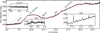 |
Fig. 1 Full JWST-MIRI MRS spectrum of CX Tau. Several emission features are labeled or shown in insets, and the continuum fit is shown in red. |
2.2 Slab modeling procedure
The molecular emission present in the spectrum is fit with 0D LTE slab models. The procedure used in this work is the same as that described in Kamp et al. (2023). We refer the reader to that work for an in-depth explanation, and provide only a summary of the most important details here.
The LTE slab models aim to reproduce the data using 3 free parameters: the line-of-sight column density N, the gas temperature T, and an emitting area A. This emitting area can be converted to an equivalent slab radius assuming A = πR2. This slab radius can be equal to the true emitting radius of the emission, but can also reflect the emission originating from an annulus further out in the disk instead. The line profiles are assumed to be Gaussian, and following Salyk et al. (2011) have a full width at half maximum of ∆V = 4.7 km s–1.
We used slab models to fit emission from 12CO2, H2O, C2H2, 13CO2,OH, and HCN, in that order. The emission from each species was fit to the data individually, after which it was subtracted to fit the emission from the next species. This process is demonstrated in the Appendix in Figs. A.1 and A.2. Since CO2, C2H2, and HCN all have Q branch features (very densely packed lines) in the MIRI wavelength range, we accounted for mutual shielding of adjacent lines for these species individually, as is described in Tabone et al. (2023).
We fit these models in the 13.5–17.5 µm region, where most molecular features are located. For H2O, we perform two separate fits in two different wavelength regions (5.5–8.5 µm and 13.5–17.5 µm), as these wavelength ranges are expected to probe different regions in the disk, and thus their excitation conditions are expected to differ (see, e.g., Gasman et al. 2023; Banzatti et al. 2023a). All slab models were convolved to the average resolving power within the fitted region (corresponding to λ/Δλ ≈ 3500 at the shortest wavelengths and to λ/Δλ ≈ 1500 at the longest wavelengths), after which they were resampled to the wavelength grid of that region using the SpectRes package (Carnall 2017). The best-fit model was obtained from a grid of models using a χ2 method as described in Grant et al. (2023), Gasman et al. (2023), and Schwarz et al. (2024). The spacing of this grid was kept consistent for most fits, where T was varied linearly between 100 and 1000 K in steps of ∆T = 22.5 K, N was varied in log-space between 1014 and 1023 cm−2 with steps of ∆ log N = 0.225. Exceptions were made for 13CO2, for which T was varied between 50 and 500 K in steps of ∆T = 11.25 K, and for OH, for which T was varied between 1000 and 3000 K in steps of ∆T = 50 K. For HCN, we restricted N between 1014 and 1021 cm–2 as the fit is very unconstrained and gave unrealistically high values otherwise. For each point in the grid, the best-fit R is determined by minimizing the reduced χ2. The χ2 fit is performed in specific spectral windows that contain important, characteristic features of the emission, avoiding contamination from other species. The average rms σ was calculated from the spectrum itself by taking the standard deviation of a relatively line-free region, for which the best-fit slab models were first subtracted. The fits to the OH and HCN emission were found to be unconstrained, and the uncertainties on the other fits are generally large. This is further discussed in Sect. 3.2 and Appendix A.
3 Results
3.1 Full spectrum
The full spectrum of CX Tau is presented in Fig. 1. The shape of the spectrum is as expected for a typical T Tauri disk: a gradual increase in flux toward the longer wavelengths, with a strong silicate feature around 10 µm. The shape of this feature has been shown to be sensitive to the average grain size in the disk, where the feature becomes broader and more flat-topped as the grains in the disk grow larger (see, e.g. Bouwman et al. 2001; Przygodda et al. 2003; Kessler-Silacci et al. 2006). As such, the silicate feature in this spectrum indicates that the dust in CX Tau is more evolved, having likely already grown to larger sizes. Additionally, several smaller “bumps” can be seen in the spectrum around 12.5, 16, 19, and 21 µm. These features are most likely caused by emission from crystalline forsterite (Olofsson et al. 2009, 2010).
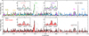 |
Fig. 2 Zoom-in of the 13.5–17.5 µm region of the CX Tau spectrum (black), together with all slab model fits to the molecular features. These models include C2H2 (yellow), HCN (orange), 12CO2 (green), 13CO2 (purple), H2O (blue), and OH (magenta). In light pink, we show a slab model demonstrating a potential detection of CO 18O. The bottom panel shows the data in black, the combined model with and without the CO 18O model in light pink and red, respectively. The red bar indicates the window in which the uncertainty was estimated. An artifact around 16.15 µm has been masked. The insets show close-ups of the regions around the 13CO2 emission feature and the (potential) CO18O feature. |
3.2 Molecular emission
The most prominent molecular feature in the spectrum of CX Tau presented in Fig. 1 is the CO2 Q branch at 15 µm. All other molecular features clearly have lower line-to-continuum ratios and as such they were likely unable to be detected with Spitzer, requiring the increased sensitivity and spectral resolution of MIRI. We detect weak H2O emission across the full spectrum, though the ro-vibrational bands at the shorter wavelengths (~5–9 µm) are slightly more prominent than the pure- rotational lines at the longer wavelengths (~ 14–24 µm). Features of 13CO2, C2H2, and HCN are also detected, and close inspection of the 13.5–17.5 µm region also reveals a potential detection of CO18O (Fig. 2 and below). OH emission is clearly detected at longer wavelengths (~ 14–24 µm) where the lines are produced by chemical pumping through the O + H2 → OH + H reaction and collisional excitation. We also find evidence of extremely excited rotational lines at shorter wavelengths (9–11 µm), known as prompt emission produced by H2O photodissociation. Emission from the high-J ro-vibrational transitions of CO at ~5 µm is not detected above 3σ. This is in line with the nondetection of CO emission reported by Anderson et al. (2024) using Keck/NIRSPEC, who instead detect narrow blue-shifted absorption indicative of a photo-evaporative wind. Finally, we also detect prominent emission from the pure-rotational transitions of H2, which show extended emission, as well as atomic emission from several hydrogen recombination lines and the forbidden [Ne II] line (see Appendix B).
To analyze the molecular emission, LTE slab model fits are used to provide an indication of the emission’s temperature, column density and emitting area (Sect. 2.2). We fit these models for the features from 12CO2, 13CO2, H2O, C2H2, HCN, and OH. Due to the weakness of most molecular features and the relatively low S/N of this spectrum, most of these emission properties are quite uncertain. For comparison, the H2O lines in CX Tau have fluxes that are ~ 100–150 times weaker than those detected in DR Tau (Temmink et al. 2024a,b). As such, we focus our analysis on detections rather than constraining parameters, and we only report on emission properties when they can be deemed robust. We discuss this further in Sect. A.1. The individual fits are shown in Appendix A in Figs. A.1, A.2, and A.3 and the χ2 maps of the constrained fits are shown in Fig. A.4.
3.2.1 12CO2, 13CO2, and CO18O
The Q branch of CO2 at 15 µm is the most prominent molecular feature detected in this source (Figs. 1 and 2).The fit to the CO2 emission indicates that the emission is tracing warm (~450 K), optically thick gas with a column density of ~8 × 1017 cm–2 at an (equivalent) emitting radius of ~0.05 au. The optically thinner isotopologue, 13CO2, is also firmly detected. The fit to this feature is less well-constrained than that for 12CO2, but it is clear from the χ2 plot (see Fig. A.4) that the emission from 13CO2 could still be marginally optically thick with its best-fit column density of ~2 × 1017 cm–2 (though this value is not very well- constrained). We find the emission to be very cold (~200 K), and it traces a larger emitting area of ~0.2 au. If we assume that the 13CO2 emission is a more reliable tracer of the total CO2 column density, we find N(CO2) = 68 × N(13CO2) ≈ 1019 cm–2.
When investigating the residuals of the fit of the 12CO2, 13CO2, H2O, C2H2, HCN, and OH emission to the 13.5– 17.5 µm region, we find a feature larger than 3σ at 15.07 µm (see the bottom panel of Fig. A.1 and Sect. A.3). This is particularly interesting as it coincides with the Q branch of CO18O. Given the bright 12CO2 emission detected in CX Tau, combined with the detection of 13CO2, a contribution from this rarer isotopologue to the observed emission could certainly be expected. We demonstrate in Fig. A.6 that there is evidence of CO18O contributing to the feature seen at 15.07 µm, as it seems too strong to be attributed solely to H2O emission. We discuss this further in Sect. A.3. We only consider this a potential detection and we thus do not fit the emission with a χ2 fit as we do for the other species in this wavelength range.
In Fig. 2, we show a CO18O model that provides a good match to the data. We assume a column density of 5 × 1016 cm−2, assuming N(13CO2)/N(CO18O) ~ 4 (from the ISM abundance ratios of 12C/13C ~68 and 16O/18O ~500, accounting for the fact that CO2 has 2 O atoms; Wilson & Rood 1994; Wilson 1999; Milam et al. 2005). The feature is quite narrow, implying a low temperature (see Fig. A.6), which is in line with our finding of a low temperature for 13CO2. The insets in Fig. 2 demonstrate the improvement that is made to the total fit when the contribution from CO18O is included. We also see that the 13CO2 and CO 18O features are similar in strength. This is in line with findings of the eXtreme UV Environments (XUE) JWST GO program (PI: Ramírez-Tannus; Ramírez-Tannus et al. 2023) , who detect these species (as well as CO17O) in an externally irradiated disk (Frediani et al., in prep.). The CO17O isotopologue is found to be the weakest of the three detected isotopologues in that work, so our data likely lack the S/N to detect it.
We investigate the difference in temperature between the 12CO2 and 13CO2 emission further in Fig. 3. This difference is especially evident when looking at the shape of their respective Q branches. The data are shown as a function of velocity, centered on the Q(8) line. This figure clearly demonstrates the sensitivity of these features to the temperature (see also Bosman et al. 2017; Grant et al. 2023), as the 12CO2 feature is clearly broader and its peak is blueshifted compared to the 13CO2 feature (which is shown in the middle and bottom panels, where the emission from 12CO2 and H2O is subtracted to isolate the feature). The bottom panel of Fig. 3 compares the 13CO2 Q branch with several slab models. In purple, the best-fitting slab model with T = 180 K is shown, and models with the same column density but T = 300 and 500 K (scaled with R to have the same peak flux) are shown in blue and red, respectively. This shows that the temperature of the 13CO2 emission can really be constrained to <300 K, as the 300 K model is already too broad.
Finally, it is interesting to test whether the 12CO2 and 13CO2 are tracing the same gas. If this were the case, we should be able to reproduce the 13CO2 feature with a slab model that has a temperature and emitting radius corresponding to the best-fit parameters of our 12CO2 model, and a column density that is 68 times smaller, following the ISM 12C / 13C ratio. The model in question is shown in green in the bottom panel of Fig. 3. Clearly, this model does not reproduce the observed 13CO2 feature. This thus indicates that the observed 12CO2 and 13CO2 emission are not tracing the same gas, likely due to the 12CO2 emission being optically thick. We also show the same test in reverse in the top panel of Fig. 3, where we show a 12CO2 model with the temperature and emitting radius of our best-fitting 13CO2 model, and with a column density 68 times larger. This model is shown in purple, and also does not reproduce all of the observed 12CO2 emission.
Thus, Fig. 3 demonstrates two things: the 13CO2 emission is colder than the 12CO2 emission and the two do not trace the same gas. This finding brings forth two possible explanations. The most straightforward explanation is that the 13CO2 emission is more optically thin, tracing deeper layers of the disk and thus lower temperatures. As the CX Tau disk has a moderate inclination (55°), this also means the emission traces further out into the disk radially, potentially explaining why the emitting radius for 13CO2 is found to be larger than that for 12CO2. In this context, the potential detection of CO 18O could also be extremely valuable, as this rarer isotopologue is even more optically thin. This could thus allow us to constrain the total CO2 column density even better, especially as the χ2 fit of the 13CO2 emission retrieves a relatively high column density and indicates that its emission may still be marginally optically thick.
However, the cold temperature of the 13CO2 emission could also indicate that it traces emission close to the CO2 snowline, possibly enhanced by radial drift and sublimating ices (see, e.g. Bosman et al. 2017). This cold component near the snowline would then also provide a part of the 12CO2 emission that is observed. This may be quantified by the purple slab model shown in the top panel of Fig. 3, which only reproduces part of the observed 12CO2 emission. Thus, the emission may be made up of both a colder and hotter component, much like what is found for H2O (e.g. Banzatti et al. 2023a; Temmink et al. 2024a; Romero-Mirza et al. 2024b). Our data lack the S/N to investigate this much further, but it motivates the study of 12CO2, 13CO2, and CO 18O emission with a more complex temperature structure in future work.
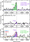 |
Fig. 3 Comparison of the 12CO2 (green) and 13CO2 (purple) Q branch shapes. Top: a zoom-in of the 12CO2 Q branch with the best-fit slab model plotted in the green shaded region. A model with the derived 13CO2 parameters is plotted in purple (see text). Middle: a zoom-in of the 13CO2 Q branch on the same vertical scale as the top panel, where the emission from 12CO2 and H2O has been subtracted. The best-fit slab model is plotted in the purple shaded region. Bottom: a further zoomin of the middle panel where the best-fit model (180 K; purple shaded region) and slab models of 300 K (blue line) and 500 K (red line) are shown. The latter two models have their emitting radius scaled to produce the same peak flux. In green, a slab model with the derived 12CO2 parameters (see text) is shown. |
3.2.2 C2H2 and HCN
As can be seen in Fig. 2, emission from C2H2 and HCN is also detected in the 13.5–17.5 µm region. Since the emission from these molecules is much weaker than that of CO2, the emission properties retrieved from our fits are quite uncertain. The emission from C2H2 is blended with H2O emission, but still detected. The fit indicates that the emission is warm and may be optically thin, and thus the column density and emitting area are poorly constrained due to their degeneracy. The HCN fit is the least constrained due to significant blending with H2O, CO2, and OH. While the emission is likely detected, its emission properties cannot be reliably determined by our fit.
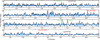 |
Fig. 4 Four panels showing a zoom-in of the 5.5–8.5 µm region of the CX Tau spectrum (black), together with the H2O slab model fits (blue). The four different panels show the regions which were used to perform the H2O χ2 fits with horizontal blue bars. |
3.2.3 H2O
H2O emission is weak, but detected. We fit it with slab models in two wavelength ranges. In the 13.5–17.5 µm region, we can clearly detect several pure-rotational H2O lines around 17.2 µm, as can be seen in Fig. 2. The best fit indicates that the H2O emission traces gas of a similar temperature (~500–600 K) and emitting radius (∼0.05 au) as the observed CO2 emission. Our best fit finds a column density of ∼1019 cm–2, which is also similar to that of CO2 if one assumes that the 13CO2 column density provides a better measure of the total CO2 column. However, if one chooses narrower fit windows (e.g. using the isolated lines suggested by Banzatti et al. 2024), a lower column density of ∼1018 cm–2 can also be retrieved. There are some weak features in the spectrum that indicate that a higher column density may be preferred, though our best-fit H2O column density of ∼1019 cm–2 may also be slightly overestimated as our data lack the S/N to properly constrain this value, and these features could also indicate the presence of hotter H2O, rather than a larger column. This is also implied by the fact that the best fit to the 13.5–17.5 µm region seems to underproduce the observed emission at shorter wavelengths (∼10–13 µm; see, e.g., Figs. B.1–B.3), indicating the potential need for a hotter component.
We fit the ro-vibrational emission at the shorter wavelengths separately from the rotational emission at 13.5–17.5 µm, as these lines are expected to trace different excitation conditions (see, e.g. Bosman et al. 2022a; Banzatti et al. 2023b). This fit is presented in Fig. 4, showing that almost all of the emission detected at these wavelengths is coming from H2O. This model indicates that this emission has a similar temperature, but is coming from a slightly smaller emitting area compared to the rotational H2O emission at 13.5–17.5 µm. This is similar to what is found in other, more in-depth studies of H2O emission (e.g. Gasman et al. 2023; Banzatti et al. 2023b; Romero-Mirza et al. 2024b; Temmink et al. 2024a). The column density is difficult to constrain due to the low S/N and the retrieved value of N > 1020 cm–2 is likely overestimated by our best fit. We also point out that this emission is likely out of LTE due to the high critical density of these transitions, leading to sub-thermal population of the levels (e.g. Meijerink et al. 2009; Bosman et al. 2022a). Still, our results show that a robust identification of H2O can be made.
At longer wavelengths (>18 µm), obtaining a constraint on the emission properties of the H2O becomes even more difficult, as the S/N ratio decreases further. As such, we do not perform a X fit in this region. We find that the slab model that was fit to the 13.5–17.5 µm region provides evidence that warm H2O emission is presumably still present in the spectrum out to ∼24 µm. We also find indications around 21 and 23 µm for a colder component of ∼200 K. This is shown in the left and middle panels of Fig. 5, where the former model is shown in light pink and the latter in light blue.
As demonstrated in Banzatti et al. (2023a) and Temmink et al. (2024a), the set of lines between 23.8 and 23.9 µm (indicated with blue and red triangles in the middle panel of Fig. 5) provides especially good evidence for the presence of this colder component to the H2O emission, as the spectrum shows that the lines indicated in blue are brighter than those indicated in red. The latter have an upper level energy that is twice as large (∼3000 K vs. ∼1500 K) and thus they rapidly grow in strength relative to the lower Eup lines when the temperature of the slab model is increased. To further demonstrate this, we show a closeup of this set of lines in the third panel of Fig. 5 where we compare our data to DR Tau, a disk for which the presence of this cold component has been firmly established (Temmink et al. 2024a). From this figure, it is clear that these lines have a similar ratio in CX Tau and thus this cold component is present in its spectrum as well.
The detection of this cold H2O component motivates the use of more complex models to better comprehend the data, for example by including multiple temperature components in a slab model fit (e.g., analysis in Pontoppidan et al. 2024; Temmink et al. 2024a) or even more complexity in the form of radial column density and temperature gradients (e.g. Kaeufer et al. 2024; Romero-Mirza et al. 2024a).
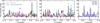 |
Fig. 5 Three panels showing a zoom-in of the 21–22 µm region, the 23–24 µm region, and the 23.75–24 µm region, respectively, of the CX Tau spectrum (black). The left and middle panels show a warm H2O slab model in light pink (the best-fit model to the 13.5–17.5 µm region), a colder (175 K) slab model in light blue and an OH slab model in magenta. Blue and red triangles denote H2O lines that demonstrate the presence of a cold H2O component in CX Tau (see text). The right panel shows the spectrum of CX Tau in black and the spectrum of DR Tau (Temmink et al. 2024a,b) in dark blue. The spectrum of DR Tau has been scaled to match the flux of the 23.87 µm line. |
3.2.4 OH
OH emission is detected at wavelengths beyond 13 µm, as already shown in Fig. 2. The fit in this region is not very well- constrained. The temperature found from the χ2 fit is very high (>1500 K), which is not representative of the physical gas temperature, but rather an effect of chemical pumping through the O + H2 → OH + H reaction, as is known to affect OH emission in this wavelength range (Tabone et al. 2021). We also detect OH emission at longer wavelengths. Due to the lower S/N in this region, we only fit this emission visually to demonstrate that it is likely also present at these wavelengths, which can be seen in Fig. 5.
Additionally, we find evidence of highly excited suprathermal rotational OH emission at shorter wavelengths (9–12 µm). These transitions originate in pure rotational states with rotational quantum numbers N as high as 44, which have upper level energies as high as ∼40 000 K. These lines are known as ‘prompt emission’ and originate from H2O photodissociation by photons in the 114–144 nm wavelength range (which includes Lyα), which brings the resulting OH molecule into a very high rotational state (van Harrevelt & van Hemert 2003; Tabone et al. 2021). The resulting cascade down the rotational ladder produces prompt emission.
One unique characteristic of prompt emission by H2O photodissociation is that the produced OH is only excited in two of the four hyperfine states that make up each rotational state (Zhou et al. 2015). Each rotational state is split by spin-orbit coupling, labeled by Ω = 1/2, 3/2 and Λ-doubling, labeled by e, f parity. H2O photodissociation only excites the Ω = 1/2, f and Ω = 3/2, e states, which are usually labeled as the A′ symmetry, with the remaining two states being labeled as the A″ symmetry.
We demonstrate in Fig. 6 the potential detection of OH prompt emission right down to 9 µm in this source. These lines have been seen with JWST/MIRI in a disk and protostellar source (Zannese et al. 2024; Neufeld et al. 2024), where the asymmetry from the preferential excitation of the A′ symmetry, uniquely indicative of OH production through H2O photodissociation, was also demonstrated. Highly excited OH emission has been observed with Spitzer in the DG Tau disk (Carr & Najita 2014) from 10 µm onward, and also more recently with MIRI in TW Hya (Henning et al. 2024).
We present our potential detection of OH prompt emission in Fig. 6 using a non-LTE OH emission model run with the thermochemical code Dust And LINes (DALI) from Tabone et al. (2024) that includes the effects of prompt emission produced by H2O photodissociation. The lines belonging to the A′ symmetry are indicated in Fig. 6 with thick, solid arrows, whereas the A″ lines are indicated with thin, dashed arrows. At short (<12 µm) wavelengths, only the A′ line pairs are detected (the individual lines are spectrally unresolved from one another at this wavelength, but resolved from the two A′′ lines), whereas the A″ line pairs are much weaker. This makes the set of lines appear as either a singlet (∼9–10 µm) or a very asymmetric doublet (∼10–12 µm). This asymmetry between the A′ and A″ lines is uniquely indicative of prompt emission produced by H2O photodissociation. We note that there are some fringe residuals in this wavelength region, which is a known issue. Still, our comparison to the depicted model provides a compelling case for this detection.
At wavelengths beyond ∼14 µm, it becomes clear that the component of the A′′ symmetry is now also present. This indicates that, aside from H2O photodissociation, chemical pumping and collisional excitation also provide an important component of the observed OH emission, as is expected for a disk (Mandell et al. 2008; Salyk et al. 2008). At this wavelength, the two A′ lines and two A″ lines are almost spectrally resolved, forming a triplet. The DALI model now closely matches the best-fit LTE slab model (shown in blue in the insets in Fig. 6) which is purely symmetrical with an equal contribution from the A′ and A″ symmetries. The DALI model still shows a very small asymmetry between the A′ and A″ lines, indicating that the preferential population of the A′′ states by H2O photodissociation affects not only the lines at shorter wavelengths, but also the triplets and quadruplets beyond 14 µm, though to a much smaller extent. Given the potential detection of OH prompt emission in our source, it stands to reason that this smaller asymmetry should be present in the emission we observe beyond 14 µm as well, but this effect is likely too small to observe.
We find evidence of OH prompt emission in CX Tau, despite the source not being a strong accretor. This could indicate some degree of dust growth and settling in the disk, allowing the UV (Lya) radiation from the star to reach deeper into the surface layers, photodissociating the H2O. The shape of the silicate feature in CX Tau is consistent with this idea. We also note that the CO2 gas, which is typically located in a similar region (e.g. Bosman et al. 2022a,b), would likely not be similarly affected, as its photodissociation rates in a radiation field dominated by Lyα have been found to be a few orders of magnitude below that of H2O (Heays et al. 2017).
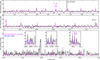 |
Fig. 6 Zoom-ins of the CX Tau spectrum (black) from 9–16.5 µm, demonstrating the potential detection of OH prompt emission. The first two panels show close-ups of the 9–11 µm region, with a non-LTE DALI model from Tabone et al. (2024) (which includes both prompt emission due to photodissociation of H2O and thermal excitation) shown in pink. The third panel shows the contributions of all slab models fit in the 13.5–17.5 µm region in gray (including OH). The DALI model is overlayed in pink. An artifact around 16.15 µm has been masked. The insets in this panel show close-ups of this model contrasted with the best-fit OH LTE slab model which is shown in blue. Lines belonging to the A′ symmetry are indicated with thick, solid pink arrows and lines belonging to the A'' symmetry are indicated with thin, dashed pink arrows. |
4 Discussion
Banzatti et al. (2020) find, based on Spitzer data, that compact dust disks typically have a higher H2O line luminosity than more extended sources. This could be attributed to these disks efficiently transporting icy pebbles inward and enriching their inner disks in H2O. CX Tau is a very compact disk with one of the highest Rgas/Rdust ratios at a value of 5 as measured by ALMA, indicating that radial drift is likely very efficient. However, our data show that the H2O emission in CX Tau is not very visually prominent in the spectrum, compared with the forest of emission lines seen in some other compact disks, such as DR Tau (Temmink et al. 2024a,b) and FZ Tau (Pontoppidan et al. 2024). Instead, it contains a strong CO2 feature, allowing us to also detect emission from 13CO2 and potentially even CO18O. As such, it is interesting to explore how CX Tau fits into this picture of compact disks and radial drift.
We begin by comparing CX Tau to the sample of disks presented in Banzatti et al. (2020), depicted in Fig. 7. Using the same spectral windows to calculate the integrated fluxes (see Najita et al. 2013), we derive an H2O flux of (4.2 ± 1.2) × 10–15 erg s–1 cm–2 and a CO2 flux of (11.5 ± 1.5) × 10–15 erg s–1 cm–2. We then convert these fluxes to a luminosity and plot them as a function of accretion luminosity, using the same value of Lacc for CX Tau as reported in Banzatti et al. (2020) for consistency. This is depicted in the left panels of Fig. 7. From this, it becomes clear that both the H2O and CO2 luminosities show a dependence on accretion luminosity. Our derived H2O line strength falls within the expected range for a source with a low accretion luminosity, whereas the CO2 flux is stronger than expected from the derived correlation by almost an order of magnitude.
The right panels of Fig. 7 show the relation between the H2O and CO2 luminosities and the dust outer radius, accounting for the correlation with Lacc. We assume that this value has an uncertainty of about 50%, in line with typical uncertainties on the conversion factors from HI line flux to accretion luminosity. Here, we once again see that the H2O line luminosity is in line with the rest of the Spitzer sample, but the CO2 luminosity stands out, being brighter than the median CO2 flux by almost an order of magnitude.
As such, it seems that the H2O flux of CX Tau falls in line with the Spitzer sample from Banzatti et al. (2020), indicating that the low accretion rate provides a likely explanation for the weakness of the warm H2O emission. For reference, both disks mentioned earlier, DR Tau and FZ Tau, have much higher accretion rates (~10–7 M⊙ yr–1; McClure 2019; Manara et al. 2023) than CX Tau (~7 ×10⁻¹⁰ M⊙ yr–1; Hartmann et al. 1998). CX Tau also has a quite moderate inclination of 55° that could contribute to its weaker emission (see, e.g. Banzatti et al. 2023b, 2024). However, while these two factors could explain the relative weakness of the H2O emission, the CO2 emission seems to have a different story. It should be similarly affected, but instead seems stronger than expected. Thus, we explore several possibilities why CX Tau could display such bright CO2 emission.
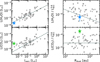 |
Fig. 7 Comparison of the CO2 and H2O luminosities derived for CX Tau (green and blue stars, respectively) to the data shown in Banzatti et al. (2020) (shown in gray). The left panels show the H2O and CO2 luminosities as a function of accretion luminosity. The right panels show the H2O and CO2 luminosities corrected for the correlation with accretion luminosity as a function of dust radius. The reported correlation between the H2O luminosity and the dust radius from Banzatti et al. (2020) is shown in the top panel, and the median CO2 luminosity is shown in the bottom panel (both shown in a gray dashed line). We note that the measurements from our data on both plots contain 1σ error bars, but these do not exceed the marker size in the left panel. |
4.1 Radial drift
First, the enhanced CO2 compared with H2O could be caused by radial drift and the resulting chemical evolution of the disk. Modeling work by Mah et al. (2023) has shown that the C/O ratio in the inner disk decreases at early times due to the inward drift of H2O-ice-rich pebbles, whose contents sublimate and enrich the gas. Then, at later times, the C/O ratio increases again due to this H2O-rich gas draining onto the central star, and the inward advection of C-rich gas from the outer disk. The work by Kalyaan et al. (2021, 2023) shows also how the delivery of H2O to the inner disk through pebble drift is sensitive to the location of potential gaps in the disk. The inner disk of CX Tau still seems to be in an O-rich phase, with H2O, CO2, and OH firmly detected, but shifts in relative CO2 /H2O abundances can already occur on a shorter timescale. Modeling work by Sellek et al. (2024) shows that the enrichment in H2O gas of the inner disk gas due to sublimation at its iceline first enhances H2O with respect to CO2, as its iceline is closest to the star. As the H2O-rich gas starts advecting inward and subsequently drains onto the star, the gas that is relatively more enriched in CO2 near the CO2 iceline is also advecting inward, eventually enriching the inner disk in CO2 instead. Mah et al. (2023) also showed that such a process proceeds faster for lower-mass stars. As CX Tau is rather low-mass (0.37 M⊙), this could mean that it has already reached a more CO2 -rich phase in its evolution, earlier than higher-mass stars of a similar age.
Sellek et al. (2024) also demonstrate that, while the inward drift of H2O-rich ice enriches the inner disk in H2O, the associated influx of dust in the inner disk may obscure the additional emission from this gas. This is due to the assumption of a lower fragmentation velocity for the dry grains inside the H2O snowline compared to icy grains outside the snowline (Blum & Wurm 2008; Gundlach & Blum 2015). As such, dust grains inside the H2O snowline fragment more easily, thereby coupling to the gas and increasing the dust opacity in the inner disk (creating a “traffic jam”, c.f. Pinilla et al. 2016). Based on these assumptions, these models predict that the column density of H2O retrieved from a synthetic spectrum may be completely insensitive to this inward drift and enrichment of the inner disk, even though the total H2O column density in this region is enhanced. The CO2 column density, however, is predicted to be much more sensitive to this evolution. This is caused by the fact that it is located further out in the disk and thus its emission is much less affected by the increase in opacity the dust drift causes, as this only affects the region inside the H2O snowline. Therefore, Sellek et al. (2024) find that the CO2 column density, and especially the CO2 /H2O column density ratio, is a good tracer of how much of it has been brought to the inner disk.
Thus, it is possible that the bright CO2 emission in CX Tau is indicative of it currently undergoing a CO2-rich phase. If the observed CO2 emission is enhanced due to the efficient drift, it would explain why it is stronger than expected from the source’s low accretion luminosity (Fig. 7). The fact that the H2O emission is not similarly enhanced could imply one of two scenarios: (1) any previous enhancement in H2O vapor mass in the inner disk has already drained onto the star, and thus the observed H2O flux is once again in line with the source’s low accretion luminosity, or (2) the H2O vapor mass in the inner disk is still enhanced due to the efficient radial drift (though past its peak), but this does not translate into an increase in observed H2O flux due to the associated influx of dust.
Naturally, it is worth noting that Sellek et al. (2024) also explore scenarios in which the sensitivity of H2O emission to drift is increased. This is done, for example, by assuming the same fragmentation velocity for icy grains and dry grains, as more recent works suggest (Gundlach et al. 2018; Musiolik & Wurm 2019), which eliminates the effect of the traffic jam. Regardless, a CO2-rich phase is still achieved. However, their models predict that the enhancement phases of H2O and CO2 are not perfectly separated in time, and an enhanced CO2 vapor mass in the inner disk likely coincides with an enhanced (though past its peak) H2O vapor mass. As such, the previous scenario described above could provide a potential explanation for the absence of a bright forest of warm H2O emission in CX Tau, where the enhancement from radial drift is hidden by the influx of dust.
There is certainly compelling evidence in the MIRI spectrum of CX Tau indicating that the radial drift of ices is important in this disk, as would be expected given its high Rgas/Rdust ratio observed with ALMA (Facchini et al. 2019). First, we report the detection of cold 13CO2 emission (Fig. 3). Modeling work by Bosman et al. (2017) has shown that the 13CO2 Q branch feature is particularly sensitive to enhancements in the CO2 abundance near the iceline created by sublimating ices. A significant enhancement can make the feature stand out prominently among the surrounding 12CO2 P branch lines, which is precisely what is observed in CX Tau. This, combined with the cold temperature the 13CO2 seems to be tracing, could indicate that there is indeed a significant volume of CO2 ice currently drifting across its iceline. The CO18O emission also shows an indication of a similarly cold temperature, so this emission may be an even better tracer of this phenomenon.
Second, we demonstrate the presence of a cold ~200 K component in the observed H2O emission (Fig. 5). The temperature of this component indicates that it potentially traces gas close to the snowline. Banzatti et al. (2023a) and Romero-Mirza et al. (2024a) demonstrate that this component is detected more strongly in the compact disks than the extended disks in their sample, which could indicate that radial drift of ices is responsible for enhancing this feature. This is further supported by the detection of a cold component in the compact disk DR Tau (Temmink et al. 2024a).
Additionally, this cold component has been further analyzed by Banzatti et al. (2024) using ratios of several diagnostic H2O lines (see Table 1 in that work) with Eup of 1500, 3600, and 6000 K. These line ratios provide useful information on the relative emission from different temperature components present in the spectrum. The 3600/6000 K line ratio mainly captures the strength of a warm (~400 K) component, whereas the 1500/3600 K line ratio captures the strength of a cold (~170–220 K) component. We measure these line ratios for CX Tau and demonstrate our results in Fig. 8. The 6000 K line is only marginally detected, so a 1σ upper limit is reported. The measured line ratios closely match the model from Banzatti et al. (2024) with a prominent cold, ~190 K component (see their Sects. 4.1 and 4.2). This demonstrates that the H2O emission in CX Tau has a significant contribution from a cold component that likely originates near the H2O snowline.
Thus, the anomalously strong CO2 emission, along with the (potential) detection of two of its weaker isotopes, could be caused by the strong radial drift in this disk creating a CO2- rich chemistry in its inner disk. The H2O emission is visually much weaker. This seems contradictory for a drift-dominated disk, however, a cold H2O component is still clearly detected, which is indicative of radial drift. The weakness of the warm H2O emission can likely be explained by its low accretion luminosity. Additionally, even if the strong radial drift has enhanced both the CO2 and H2O vapor mass in the inner disk, the associated influx of dust could potentially explain why an enhancement in observed flux is only seen in CO2, and not in H2O. The relatively weak C2H2 and HCN emission from the disk is also consistent with this scenario, as these species are likely more sensitive to CX Tau’s low accretion luminosity than a process like radial drift.
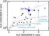 |
Fig. 8 H2O diagnostic diagram from Banzatti et al. (2024), adapted to include the measured line ratios for CX Tau. Data points from Banzatti et al. (2024) (excluding data points with upper/lower limits) are indicated with black circles and the data point for CX Tau is indicated with a blue star. Three models from Banzatti et al. (2024) are shown: the model with a hot (850 K) and warm (400 K; optically thick) component is shown as a gray solid line (labeled “H + W (TK)”), the model with a hot (850 K) and warm (400 K; optically thin) component is shown as a dashed, gray line (labeled “H + W”), and the model with a hot (850 K), warm (400 K), and cold (190 K) component is shown as a dashed, light gray line (labeled “H + W + C”). |
4.2 A small inner cavity
An alternate explanation for the bright CO2 emission that has been proposed in previous work is the presence of a small inner cavity. This argument was put forth to potentially explain the bright CO2 observed in GW Lup (Grant et al. 2023), and it was tested with Dust And LINes (DALI) thermo-chemical models in Vlasblom et al. (2024). The latter work shows that the presence of a small, inner cavity can suppress the H2O emission and enhance that of CO2. The work also shows that a source like CX Tau, with a luminosity of L* = 0.2 L⊙, would need a cavity of approximately 2 au in radius (thus 4 au in diameter; see Appendix B in that work). This is below the resolution of the current highest angular resolution ALMA observations available (Facchini et al. 2019, with a resolution of 5 au), and thus the presence of such a cavity cannot currently be confirmed or ruled out. Facchini et al. (2019) do calculate an upper limit on the size of a possible inner cavity from the intensity profile and find an upper limit of 0.54 au. That would seem to rule out our proposed cavity of 2 au, but we argue that a 2 au cavity could still be completely hidden from view in these observations, especially if the cavity is not fully depleted in dust (Vlasblom et al. 2024 show that a depletion in gas and dust of at least a factor 104 is needed). Thus, even higher angular resolution ALMA observations, combined with super-resolution techniques, would be needed to truly confirm or rule out the presence of an inner cavity.
The presence of such a cavity does raise quite a few concerns when combined with our findings in this work. For one, we find very small emitting radii for most of our species, on the order of ~0.05 au. In Sect. 2.2, we stress that the emitting area is parameterized by a radius, but that the emission can also originate from a thin annulus further out. We can contrast this with the 2D thermochemical models presented in Vlasblom et al. (2024), which do show that the emission originates from a very thin annulus once the cavity is made large enough to enhance the CO2 emission sufficiently with respect to the H2O emission (see, e.g. Fig. 2 and Appendices A and B in that work), though perhaps not quite to the extent our derived emitting area would imply.
Similarly, one may wonder if such a cavity around a relatively faint star could even produce temperatures at the cavity wall that are hot enough to match our observed emission of ~500 K. The thermochemical model by Vlasblom et al. (2024) finds that temperatures of 500–600 K are reached within the molecular emitting region at the cavity wall, so this seems to be possible. We also refer back to CX Tau’s moderate inclination of 55° here. With this, the cavity wall would be directly exposed to the observer, so the high temperatures at the very inner edge of the cavity wall would be directly visible.
Finally, one should also consider that a 2 au cavity in the inner disk likely impacts the SED quite strongly. CX Tau actually has an interesting history of having once been classified as a transition disk based on the (lack of) near-IR excess in its SED (Najita et al. 2007). However, when common color criteria are used, such as in Furlan et al. (2011), CX Tau does not qualify. Theoretical work shows that IR spectral indices n13–30 > 0 are likely a result of dust cavities (e.g. Woitke et al. 2016; Ballering & Eisner 2019). Banzatti et al. (2020) report an n13–30 index of – 0.15 for CX Tau. Nevertheless, their sample contains some disks with n13–30 < 0 that still have an inner cavity detected (which, interestingly, are sources with similar inclinations to CX Tau, as seen by the red markers in, e.g., their Figs. 6 and 9), indicating that the SED of CX Tau does seem to allow for the presence of a small cavity.
To conclude, the presence of a small, inner cavity in CX Tau cannot yet be ruled out. However, the scenario does raise some valid concerns, as modeling has found that the needed cavity size (2 au) is relatively large, given CX Tau’s small dust radius and low luminosity. Thus, while a small cavity could be responsible for the enhanced CO2 emission, the scenario of enhancement by radial drift seems preferred.
4.3 Gas-to-dust ratio and disk temperature
Finally, Vlasblom et al. (2024) show that a large amount of dust in the inner regions could also enhance CO2 emission relative to H2O, as shown from their models with a lower gas-to-dust ratio. This dust could be brought to the inner disk by radial drift, and subsequently could be stirred up into the IR emitting layers of the disk by turbulence, clouding the region. It has been shown that the H2O emission detected in disks with Spitzer, which are thus disks with much brighter H2O emission than CX Tau, is likely coming from a layer with a gas-to-dust ratio that is locally enhanced by 1–2 orders of magnitude (Meijerink et al. 2009; Bosman et al. 2022a). An enhancement in the amount of dust in these layers could thus obscure this emission, as is also seen in Woitke et al. (2018) and Greenwood et al. (2019). Furthermore, Bosman et al. (2023) speculate that the features from CO2 could remain visible due to IR pumping, though in-depth modeling would be needed to confirm this. The dust would also make the IR emitting layers cooler. As CO2 preferentially forms from OH over H2O at temperatures below ~300 K (Charnley 1997; van Dishoeck et al. 2013; Walsh et al. 2015), this means that more CO2 could be formed in a cooler disk with more dust than in a hotter, more settled disk.
This scenario is proposed by Bosman et al. (2023) to explain the bright CO2 emission observed in IM Lup, another source that seems to have peculiarly bright CO2 emission, just like GW Lup and CX Tau. Bosman et al. (2021, 2023) demonstrate a pile-up of dust in the inner disk of IM Lup, pointing to a low gas-to-dust ratio and high turbulence in this region. This scenario may thus provide another alternate explanation for the bright CO2 emission in CX Tau, though one would need to investigate further whether the source shows similar evidence for a low gas-to-dust ratio in the inner disk.
5 Conclusions
We present JWST MIRI/MRS observations of the disk around CX Tau, a compact, drift-dominated disk whose IR molecular features have not been analyzed before. Our main conclusions are as follows:
We detect bright emission from CO2 and much weaker features from H2O, 13CO2, C2H2, HCN, and OH for the first time in this disk. We constrain their properties using 0D LTE slab models. All of these weaker features have line-to- continuum ratios that are too small for them to have been detected previously, demonstrating the vast improvement in the detection of such faint emission that JWST has brought;
We find the 12CO2 to be optically thick, tracing a temperature of ~450 K at an (equivalent) emitting radius of ~0.05 au, whereas the 13CO2 traces much colder temperatures (~200 K) and a larger emitting area.
We also report a potential detection of the even rarer isotopologue, CO18O, in the disk;
We detect warm, ~500 K, pure rotational emission from H2O, as well as ro-vibrational emission that traces slightly warmer gas. We also find evidence for a colder, ~200 K, component;
We report a potential detection of highly excited rotational OH lines between 9 and 12 µm which are caused by H2O photodissociation, as well as emission caused by chemical pumping and collisional excitation at longer wavelengths;
We detect 4 pure rotational H2 lines for which we find tentative evidence that this emission is extended, based on analysis of the PSF;
The strong radial drift, known to be present in this source, could be responsible for the observed CO2 -rich chemistry. The drift could have increased the CO2 vapor mass in the inner disk, enhancing the observed emission. As it is located further out in the disk than H2O, the CO2 emission would be less affected by any enhancements in dust opacity from the radial drift;
The comparatively weaker H2O emission could be explained by the source’s low accretion luminosity, assuming that any enhancement in H2O vapor mass by drift has already advected onto the star. Alternatively, the H2O vapor mass could still be somewhat enhanced in the inner disk, but it is possible that this would not translate into an increased flux due to the increased dust opacity within the H2O snowline;
The observed cold 13CO2 and H2O support the idea that radial drift of ices is important for the observed IR emission in this disk;
Alternatively, the bright CO2 emission and relatively weaker H2O emission could hint at the presence of previously unrevealed substructures in the disk in the form of a small, inner cavity with a size of roughly 2 au in radius. Higher angular resolution ALMA observations are needed to confirm this.
This work has demonstrated how JWST can give us a much deeper insight into how disk structure and radial drift of ices could produce the CO2 -rich chemistry observed in this drift- dominated disk on scales where terrestrial planets may be forming. To understand these processes and their link to disk chemistry even better, it will be interesting to investigate these trends in a larger sample, for example in a sample of compact, drift-dominated disks (e.g. expanding upon the work by Banzatti et al. 2023a), or in a sample of CO2-bright disks.
Acknowledgements
We thank the referee for their detailed comments which helped improve this paper. This work is based on observations made with the NASA/ESA/CSA James Webb Space Telescope. The data were obtained from the Mikulski Archive for Space Telescopes at the Space Telescope Science Institute, which is operated by the Association of Universities for Research in Astronomy, Inc., under NASA contract NAS 5-03127 for JWST. These observations are associated with program #1282. The following National and International Funding Agencies funded and supported the MIRI development: NASA; ESA; Belgian Science Policy Office (BELSPO); Centre Nationale d’Etudes Spa- tiales (CNES); Danish National Space Centre; Deutsches Zentrum fur Luft- und Raumfahrt (DLR); Enterprise Ireland; Ministerio de Economía y Com- petividad; Netherlands Research School for Astronomy (NOVA); Netherlands Organisation for Scientific Research (NWO); Science and Technology Facilities Council; Swiss Space Office; Swedish National Space Agency; and UK Space Agency. M.V., M.T., and A.D.S. acknowledge support from the ERC grant 101019751 MOLDISK. A.C.G. acknowledges from PRIN-MUR 2022 20228JPA3A “The path to star and planet formation in the JWST era (PATH)” funded by NextGeneration EU and by INAF-GoG 2022 “NIR-dark Accretion Outbursts in Massive Young stellar objects (NAOMY)” and Large Grant INAF 2022 “YSOs Outflows, Disks and Accretion: toward a global framework for the evolution of planet forming systems (YODA)”. D.B. is funded by the Spanish MCIN/AEI/10.13039/501100011033 grant PID2019-107061GB-C61. G.P. gratefully acknowledges support from the Max Planck Society. E.v.D. acknowledges support from the ERC grant 101019751 MOLDISK and the Danish National Research Foundation through the Center of Excellence “InterCat” (DNRF150). T.H. and K.S. acknowledge support from the European Research Council under the Horizon 2020 Framework Program via the ERC Advanced Grant Origins 83 24 28. I.K., A.M.A., and E.v.D. acknowledge support from grant TOP-1 614.001.751 from the Dutch Research Council (NWO). I.K. acknowledges funding from H2020-MSCA-ITN-2019, grant no. 860470 (CHAMELEON). B.T. is a Laureate of the Paris Region fellowship program, which is supported by the Ile- de-France Region and has received funding under the Horizon 2020 innovation framework program and Marie Sklodowska-Curie grant agreement No. 945298. V.C. acknowledges funding from the Belgian F.R.S.-FNRS. D.G. thanks the Belgian Federal Science Policy Office (BELSPO) for the provision of financial support in the framework of the PRODEX Programme of the European Space Agency (ESA).
Appendix A Slab fitting routine
We show here several additional figures from our slab fitting routine. In Figs. A.1, A.2, and A.3, we show the six individual fits performed in the 13.5 to 17.5 µm region, and we discuss the uncertainties on the fitting routine below. In Fig. A.4 we show theχ2 plots that result from the CO2,13CO2, C2H2, and H2O fits (as the OH and HCN fits are found to be unconstrained). In Fig. A.6 we discuss the residuals in the fit which potentially belongs to emission from CO18O.
A.1 Uncertainties on the step-by-step fitting routine
As stated in Sect. 3.2, the retrieved fit parameters are quite uncertain due to the relatively low S/N of the spectrum and the weakness of the molecular emission. In the 13.5-17.5 µm range, weak features from 12CO2,13CO2, H2O, C2H2, HCN, and OH all overlap, making the emission complicated to fit. We do this by fitting the emission of each molecule individually, after which it is subtracted from the spectrum and the next species is fit. It is also possible to fit the emission from all species simultaneously using an MCMC routine (e.g., as done in Grant et al. 2024). We provide a comparison between the two methods in Fig. A.5, which demonstrates that the two produce similar conclusions. We also stress that our main results do not rely on the emission properties being constrained with large accuracy.
As demonstrated in Figs. A.1 and A.2, we begin by fitting the most prominent feature: 12CO2. After that, we fit the H2O emission, of which the features span the entire fitted wavelength range. After that, we fit the remaining molecular features from C2H2, 13CO2, OH, and HCN in that order. The selection of the windows in which the fits are performed can significantly impact the results of this method. After all, a lot of the weak molecular features have significant overlap with other species. As such, we are careful to select features that are as isolated as possible from contaminating emission. This is particularly important for 12CO2 and H2O. The remaining species have detected features only in more specific wavelength ranges, thus strongly limiting the possible isolated features that can be selected. Thus, we focus on avoiding their features in the 12CO2 and H2O fit windows.
For H2O, we find that the retrieved column density is particularly sensitive to the selection of the fit windows: enlarging the windows allows for more weak features at the noise level to be included, increasing the column density. Additionally, it is important that our fit windows contain lines of different upper level energies Eup and Einstein A-coefficients Aij, to avoid a potential bias in the fit. This is especially important for H2O, for which lines with a large diversity in Eup and Aij are present in this wavelength range (see, e.g., Figs. 14 and 15 in Pontoppidan et al. 2024).
As such, we define our fit windows as follows: for 12CO2, our windows contain its Q branch, several isolated P and R branch lines, as well as the hot bands. For H2O, we select the detected, unblended lines from Tables 6 & 7 in Banzatti et al. (2024) in addition to a few other clearly detected features, for example at 17.2 µm. The remaining species have well-detected features only in more specific wavelength ranges. For OH, we make sure to cover all triplets seen in the 13.5-17.5 µm range, avoiding lines blended with H2O. For 13CO2, C2H2, and HCN we cover their entire Q branches in our windows, but we do not cover much more as these are the only prominent features we can detect, aside from the HCN hot band at 14.3 µm. The windows are indicated in Figs. A.1 and A.2 with horizontal bars.
Finally, the specific order in which these six species are fit may also impact the fit results. The features from C2H2, 13CO2, OH, and HCN do not overlap with one another significantly, so the order in which they are fit does not have a significant impact. We do find, however, that it is important to remove the contribution from 12CO2 emission before the H2O, as the latter is much weaker and thus blended with the 12CO2 P and R branch lines. We also find that the H2O emission is significantly blended with the C2H2 and HCN features, making it important to fit the H2O before those two species. However, selecting isolated fit windows for each species can mitigate this, as evidenced by the fact that the MCMC method, which fits all species simultaneously, produces similar conclusions as the step-by-step method.
The best-fit parameters of the 12CO2,13CO2, C2H2, and H2O fits and any degeneracies between them can be seen in Fig. A.4. We exclude the χ2 maps from OH, HCN, and H2O at 5.5-8.5 µm. The HCN and OH fits are unconstrained and therefore do not provide a reliable indication of the emission properties. The H2O fit at short wavelengths (as well as the OH fit) may be affected by non-LTE effects and the retrieved column density is likely overestimated. For the other species, the parameters are more constrained. However, the uncertainties on these values are still large and thus we do not report on the best-fitting parameters in much detail. 12CO2 is the only exception to this, being the brightest emission feature. Still, we do caution that the hot band at 16.2 µm is affected by an artifact, which may have affected the estimation of our fit results slightly. For the other species, we can only derive the temperature within ~ 100-200 K and the column density within ~1-2 dex.
A.2 Comparison with the MCMC routine
We fit the emission from 12CO2, 13CO2, H2O, C2H2,HCN, and OH between 13.5 and 17.5 µm simultaneously using an MCMC routine, following the method described in Grant et al. (2024). We compare the best-fit results from this method to the best fits from our step-by-step routine in Fig. A.5. The conclusions derived from both methods generally agree, suggesting that the step-by-step fitting is not significantly biased by the order in which we fit the molecules. The 12CO2 parameters are the most well-constrained. For H2O, the temperature and emitting area agree well, but the derived column density from the MCMC is higher (> 1020 cm−2). This is likely due to the inclusion of weak features at the noise level, as we performed the fit over the whole wavelength range at once rather than limiting it to specific spectral features. As such, the MCMC method may be better suited for fitting the H2O emission in higher S/N sources rather than a low S/N source like CX Tau.
The MCMC finds both the C2H2 and 13CO2 emission to be optically thin and thus the column density and emitting area are completely degenerate. For C2H2, this agrees with our step-by-step fitting. We stress that the MCMC was allowed to explore a broader parameter space and the slight difference between our results and the MCMC is due to this degeneracy. For 13CO2, the MCMC seems to favor a more optically thin solution than our step-by-step routine, though this parameter is poorly constrained. The cold temperature of the 13CO2 emission, however, is agreed upon by both methods.
A.3 Residuals
We demonstrate in Figs. A.1 and A.2 that most of the residuals in the 13.5-17.5 µm region fall within 3σ after all of the fits are subtracted. The residuals at the shorter wavelengths, between 13.5 and 16 µm, are likely affected by the heavy blending of weak features from CO2, C2H2, HCN, H2O, and OH, perhaps explaining their observed structure. It is also possible that some weak H2O features from hotter emission are unaccounted for in our single-temperature slab fit. In fact, the features depicted in Fig. A.2 at 16.9 and 17.35 µm coincide with low Eup H2O lines, and can thus likely be attributed to a colder component of H2O, indicating that there are multiple temperature components present in this wavelength range. However, as also mentioned in Sect. 3.2.3, we do not intend to characterize the emission properties in that much detail in this work, and as such we only present a single-temperature slab fit.
Aside from that, one residual feature stands out beyond 3σ: a peak at 15.07 µm. This feature is of particular interest, as it coincides with the Q branch of CO18O. We aim to explore the possibility of a detection with Fig. A.6. Here, we compare our data for CX Tau to two H2O-rich disks, DR Tau (Temmink et al. 2024a,b) and DF Tau (Grant et al. 2024). These disks contain evidence for hotter and colder water components that are not included within our single-component fit. We rescale the spectra for these two disks to the H2O feature at 15.17 µm. In the left panel of the figure, we show the CX Tau spectrum with the CO2 emission subtracted in black, the best-fit H2O model in light blue, a 200 K CO18O model in yellow, and the combination of the two models (H2O and CO18O) in red. We compare this to the two H2O-rich sources, which demonstrates that the 15.07 µm feature seems to stand out abnormally in CX Tau. A comparison to the neighboring 15.17 µm H2O feature makes this especially clear.
DR Tau and DF Tau both show H2O emission at these two wavelengths, indicating that at least some of the 15.07 µm feature can be ascribed to H2O. It is possible that our current best fit lacks some high-energy H2O emission, as it seems too narrow compared to the emission seen in DR Tau and DF Tau. However, it is also clear that the 15.17 µm lines are much stronger than the 15.07 µm lines in DR Tau and DF Tau, whereas the opposite is true in CX Tau. Thus, if one tries to fit a high temperature H2O model that fills in the 15.07 µm feature to the extent that is seen in CX Tau, the surrounding H2O lines are massively overproduced. This lends credit to the idea that at least some of the prominence of this feature is due to a contribution of CO18O emission, not solely H2O.
This is supported by the CO18O models shown in the right panel of Fig. A.6. Here, we show a close-up of the residuals after all fits are subtracted (so not only CO2, like in the left panel) and we plot three CO18O models at 200, 300, and 400 K, scaled with R to fit the feature. We assume a column density of N = 5 × 1016 cm−2 for these models, which is the expected column density assuming N(13CO2)/N(CO18O) ~ 4 (from the ISM abundance ratios of 12C/13C ~68 and 16O/18O ~500, accounting for the fact that CO2 has 2 O atoms; Wilson & Rood 1994; Wilson 1999; Milam et al. 2005). The coldest model fits the feature very nicely. This would be in line with the cold (~200 K) temperature found for the 13CO2 feature. However, we do wish to stress that this residual, as it is depicted in the right panel, could also contain some high-energy H2O emission that is lacking from our best-fit model, as the comparison with DR Tau and DF Tau suggests. This could bias the determination of the temperature. Still, the prominence of the 15.07 µm feature suggests it should not be attributed solely to H2O emission, and Fig. A.6 demonstrates that a contribution from CO18O is certainly possible.
 |
Fig. A.1 Zoom-in of the 13.5-15.5 µm region of the CX Tau spectrum (black), where all individual slab model fits are shown. Horizontal bars indicate which spectral windows were used for the χ2 fit, and each panel indicates which other models were removed from the spectrum before the fit was performed, to avoid contamination from other molecules. The final panel shows the residuals after all fits are subtracted, with the shaded region indicating that most residuals fall below 3σ. We note the difference in scale on the y axis between the top panel and the rest. |
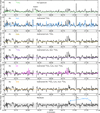 |
Fig. A.2 Zoom-in of the 15.5-17.5 µm region of the CX Tau spectrum (black), where all individual slab model fits are shown. Horizontal bars indicate which spectral windows were used for the χ2 fit, and each panel indicates which other models were removed from the spectrum before the fit was performed, to avoid contamination from other molecules. The final panel shows the residuals after all fits are subtracted, with the shaded region indicating that most residuals fall below 3σ. An artifact around 16.15 µm has been masked in all panels. We also note the difference in scale on the y axis between the top panel and the rest. |
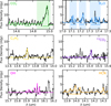 |
Fig. A.3 Various zoom-ins of Figs. A.1 and A.2, to depict the goodness of the individual slab fits. Horizontal bars indicate which spectral windows were used for the χ2 fit. The vertical shaded regions indicate the windows used to calculate the CO2 and H2O fluxes, following Salyk et al. (2011) and Najita et al. (2013). |
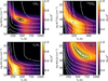 |
Fig. A.4 χ2 maps for the 12CO2,13CO2, C2H2, and H2O slab model fits in the 13.5-17.5 µm wavelength range. The color-scale indicates |


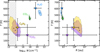 |
Fig. A.5 Comparison between the MCMC routine and our step-by-step fitting routine. The stars represent the best-fit results from the step-by-step fits with 1 σ errorbars. The small circles represent the best-fit results from the MCMC and the colored area represents a 3 σ confidence. The hatched area in the left panel demonstrates the parameter space that is covered by the MCMC, but not the step-by-step routine. |
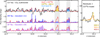 |
Fig. A.6 Zoom-in of the CX Tau spectrum around the 15.07 µm feature which stands out in our residuals in Fig. A.1. Left: The CX Tau spectrum with the best-fit CO2 model subtracted is shown in black, the best-fit H2O model is shown in light blue, a 200 K, N = 1016 cm−2 CO18O model shown in yellow and the combined H2O and CO18O model is shown in red. The spectra of DR Tau and DF Tau (Temmink et al. 2024a,b; Grant et al. 2024), rescaled to the 15.17 µm H2O feature in CX Tau, are shown in dark blue and purple, respectively. Right: The CX Tau spectrum with all best-fit models (12CO2,13CO2, H2O, C2H2, HCN, and OH) subtracted is shown in black. Three CO18O models with N = 1016 cm−2 and different temperatures are shown in yellow, orange, and brown. |
Appendix B Other emission features
B.1 HI
We detect several atomic hydrogen recombination lines that have a principal quantum number of the lower energy levels of 5 or 6 (Pfund and Humphreys series), and a tentatively detect a few from the next higher series. An overview is presented in Fig. B.1. The brightest H line detected is the Pfα line at 7.46 µm, but the Huα (HI 7-6) line at 12.37 µm is also detected. The flux of this line has been shown by Rigliaco et al. (2015) to have an empirical correlation with a source’s accretion luminosity Lacc, which is as follows:
 (B.1)
(B.1)
Then, following Gullbring et al. (1998), the derived Lacc can be used to calculate the mass accretion rate Ṁacc:
 (B.2)
(B.2)
Here, M* = 0.37M⊙ is the stellar mass (Simon et al. 2017), Rin = 5R*, (Herczeg & Hillenbrand 2008) is the radius at which the stellar magnetosphere truncates the accreting gas, and R* = 1.2R⊙ is the stellar radius. The stellar radius is calculated using the Stefan-Boltzmann relation  , where the stellar luminosity L*= 0.2 L⊙ and the effective temperature is Teff = 3483 K (Herczeg & Hillenbrand 2014).
We measure the flux of the HI (7-6) line by fitting a Gaussian to it. A similar analysis was performed in Franceschi et al. (2024), where this line was found to be blended with the HI (11-8) line. We annotate the position of this line in Fig. B.1 to show that it is not detected in our data, hence we do not expect contribution from this line to impact our results. Calculating the accretion luminosity yields Lacc = (1.9 ± 1.3) × 10−3L⊙. Using this value to then calculate the mass accretion rate yields Ṁacc = (2.6 ± 1.9) × 10−10M⊙ yr−1. Both of these values are in good agreement with literature values (within a factor 2-3, see, e.g., Hartmann et al. 1998; Fang et al. 2018).
B.2 H2
Several pure-rotational H2 lines are detected in CX Tau. As shown in Fig. B.2, the 0-0 S(1), S(2), S(3), and S(5) lines are firmly detected. We find evidence that the emission from these lines is extended. This is demonstrated in Anderson et al. (2024), who show that this emission extends out to ~500 au, much further than the CO gas disk detected with ALMA (Facchini et al. 2019). It is possible that some of the H2 emission detected on source traces the disk itself, as H2 should naturally be abundant there. Additionally, the shape of the silicate feature indicates that the dust is more evolved and therefore perhaps less opaque, potentially aiding in such a detection, as was found to be the case in Franceschi et al. (2024). However, H2 emission is also a very common tracer of disk winds. We also detect [Ne II] in our source, which Anderson et al. (2024) also demonstrate to be extended. Additionally, the work presents a detection of blue-shifted CO absorption with Keck/NIRSPEC. All of this indicates that CX Tau likely has a photo-evaporative wind.
B.3 Neon
Aside from hydrogen, emission from neon is also detected in CX Tau. As presented in Fig. B.3, we clearly detect the [Ne II] line at 12.8 µm, and close inspection of the 15.5 µm region does reveal some emission that could potentially be associated with the [Ne III] line, but could also be slightly underproduced H2O emission (combined contributions from 12CO2,13CO2,H2O,OH,C2H2, and HCN are shown in red). We obtain the line flux of the [Ne II] line by fitting a Gaussian profile and we derive a 3 σ upper limit on the [Ne III] line flux, after which we divide the two to obtain a 3 σ upper limit on the [Ne III]-to-[Ne II] ratio. This yields a value of 0.5.
Theoretical work has shown that this value can indicate whether X-rays or extreme ultraviolet (EUV) radiation produces the emission. Hollenbach & Gorti (2009) showed that EUV radiation produces [Ne III]-to-[Ne II] ratios > 1, whereas Glassgold et al. (2007) and Meijerink et al. (2008) showed that X-rays produce [Ne III]-to-[Ne II] ratios of approximately 0.1. This difference is mainly caused by the difference in depth to which X-ray or EUV photons can penetrate the disk. X-ray photons penetrate further, into a layer that contains mostly neutral H. This leads to a very effective charge exchange between Ne2+ and H converting a lot of the Ne2+ into Ne+, thus leading to a low [Ne III]-to-[Ne II] ratio. EUV photons, however, cannot penetrate that deeply into the disk, only reaching a layer that is still mostly ionized, containing much less neutral H. As such, the charge exchange converting Ne2+ into Ne+ is much less efficient, leading to much higher [Ne III]-to-[Ne II] ratios, typically higher than 1.
Our derived upper limit on the [Ne III]-to-[Ne II] ratio is less than 1, indicating that the former case, where the neon ions are predominately produced by X-rays, is more likely to be responsible for the observed Ne emission. This is in line with typical findings for T Tauri stars, such as previous results from Spitzer (Szulágyi et al. 2012; Espaillat et al. 2013) and more recent JWST results (Espaillat et al. 2023). However, Anderson et al. (2024) point out that the relative line fluxes of the H2 S(1) and S(3) lines are more consistent with EUV excitation, rather than X-rays. Our derived [Ne III]-to-[Ne II] ratio (while more consistent with X-ray excitation) could indicate that CX Tau is an in-between case, making it an interesting subject for further study. We do not detect any other atomic emission from, for example, argon or iron.
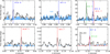 |
Fig. B.1 Zoom-ins of the CX Tau spectrum (black) around various possible detections of H lines. We show the best-fit ro-vibrational H2O model (the best fit to the 5.5-8.5 µm region) in all panels containing lines below 10 µm and the best-fit rotational model (the best fit to the 13.5-17.5 µm region) in all panels containing lines at longer wavelengths. These H2O slab models are shown in blue, and solid vertical lines indicate the central wavelengths of the H lines, where the nlow = 5 (Paschen) series is shown in green, the nlow = 6 (Humphreys) series is shown in blue, and the nlow = 7 series is shown in red. |
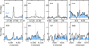 |
Fig. B.2 Zoom-ins of the CX Tau spectrum (black) at the locations of the eight pure-rotational H2 lines in the MIRI/MRS wavelength range. We show the best-fit ro-vibrational H2O model (the best fit to the 5.5-8.5 µm region) in all panels containing lines below 10 µm and the best-fit rotational model (the best fit to the 13.5-17.5 µm region) in all panels containing lines at longer wavelengths. These H2O slab models are shown in blue. |
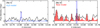 |
Fig. B.3 Zoom-ins of the CX Tau spectrum (black) around the [Ne II] and [Ne III] lines. In the left panel, a Gaussian fit to the [Ne II] line is shown in dark blue together with the best-fit H2O model from the 13.5-17.5 µm range in light blue. In the right panel, the combined model containing 12CO2,13CO2, HCN, C2H2, H2O, and OH is shown in red. A blue dashed line indicates the position of the [Ne III] line and the shaded region surrounding it indicates the region in which the upper limit on its flux is derived. |
References
- Anderson, A. R., Williams, J. P., Blake, G. A., et al. 2024, ApJ, 997, 213 [NASA ADS] [CrossRef] [Google Scholar]
- Andrews, S. M., Huang, J., Pérez, L. M., et al. 2018, ApJ, 869, L41 [NASA ADS] [CrossRef] [Google Scholar]
- Ansdell, M., Williams, J. P., Trapman, L., et al. 2018, ApJ, 859, 21 [NASA ADS] [CrossRef] [Google Scholar]
- Arabhavi, A. M., Kamp, I., Henning, T., et al. 2024, Science, 384, 1086 [NASA ADS] [CrossRef] [Google Scholar]
- Argyriou, I., Glasse, A., Law, D. R., et al. 2023, A&A, 675, A111 [NASA ADS] [CrossRef] [EDP Sciences] [Google Scholar]
- Ballering, N. P., & Eisner, J. A. 2019, AJ, 157, 144 [Google Scholar]
- Banzatti, A., Pascucci, I., Bosman, A. D., et al. 2020, ApJ, 903, 124 [NASA ADS] [CrossRef] [Google Scholar]
- Banzatti, A., Pontoppidan, K. M., Carr, J. S., et al. 2023a, ApJ, 957, L22 [NASA ADS] [CrossRef] [Google Scholar]
- Banzatti, A., Pontoppidan, K. M., Pére Chávez, J., et al. 2023b, AJ, 165, 72 [CrossRef] [Google Scholar]
- Banzatti, A., Salyk, C., Pontoppidan, K. M., et al. 2024, arXiv e-prints [arXiv:2409.16255] [Google Scholar]
- Bitsch, B., & Mah, J. 2023, A&A, 679, A11 [NASA ADS] [CrossRef] [EDP Sciences] [Google Scholar]
- Blum, J., & Wurm, G. 2008, ARA&A, 46, 21 [Google Scholar]
- Booth, R. A., Clarke, C. J., Madhusudhan, N., & Ilee, J. D. 2017, MNRAS, 469, 3994 [Google Scholar]
- Bosman, A. D., Bruderer, S., & van Dishoeck, E. F. 2017, A&A, 601, A36 [NASA ADS] [CrossRef] [EDP Sciences] [Google Scholar]
- Bosman, A. D., Bergin, E. A., Loomis, R. A., et al. 2021, ApJS, 257, 15 [NASA ADS] [CrossRef] [Google Scholar]
- Bosman, A. D., Bergin, E. A., Calahan, J., & Duval, S. E. 2022a, ApJ, 930, L26 [NASA ADS] [CrossRef] [Google Scholar]
- Bosman, A. D., Bergin, E. A., Calahan, J. K., & Duval, S. E. 2022b, ApJ, 933, L40 [NASA ADS] [CrossRef] [Google Scholar]
- Bosman, A. D., Appelgren, J., Bergin, E. A., Lambrechts, M., & Johansen, A. 2023, ApJ, 944, L53 [NASA ADS] [CrossRef] [Google Scholar]
- Bouwman, J., Meeus, G., de Koter, A., et al. 2001, A&A, 375, 950 [NASA ADS] [CrossRef] [EDP Sciences] [Google Scholar]
- Bushouse, H., Eisenhamer, J., Dencheva, N., et al. 2023, JWST Calibration Pipeline [Google Scholar]
- Carnall, A. C. 2017, arXiv e-prints [arXiv:1705.05165] [Google Scholar]
- Carr, J. S., & Najita, J. R. 2014, ApJ, 788, 66 [NASA ADS] [CrossRef] [Google Scholar]
- Charnley, S. B. 1997, ApJ, 481, 396 [NASA ADS] [CrossRef] [Google Scholar]
- Christiaens, V., Gonzalez, C., Farkas, R., et al. 2023, J. Open Source Softw., 8, 4774 [NASA ADS] [CrossRef] [Google Scholar]
- Christiaens, V., Samland, M., Gasman, D., Temmink, M., & Perotti, G. 2024, MINDS: Hybrid pipeline for the reduction of JWST/MIRI-MRS data, Astrophysics Source Code Library [record ascl:2403.007] [Google Scholar]
- Cieza, L. A., Ruíz-Rodríguez, D., Hales, A., et al. 2019, MNRAS, 482, 698 [Google Scholar]
- Dawson, R. I., & Johnson, J. A. 2018, ARA&A, 56, 175 [Google Scholar]
- Erb, D. 2022, pybaselines: A Python library of algorithms for the baseline correction of experimental data [Google Scholar]
- Espaillat, C., Ingleby, L., Furlan, E., et al. 2013, ApJ, 762, 62 [NASA ADS] [CrossRef] [Google Scholar]
- Espaillat, C. C., Thanathibodee, T., Pittman, C. V., et al. 2023, ApJ, 958, L4 [NASA ADS] [CrossRef] [Google Scholar]
- Facchini, S., Birnstiel, T., Bruderer, S., & van Dishoeck, E. F. 2017, A&A, 605, A16 [NASA ADS] [CrossRef] [EDP Sciences] [Google Scholar]
- Facchini, S., van Dishoeck, E. F., Manara, C. F., et al. 2019, A&A, 626, L2 [NASA ADS] [CrossRef] [EDP Sciences] [Google Scholar]
- Fang, M., Pascucci, I., Edwards, S., et al. 2018, ApJ, 868, 28 [NASA ADS] [CrossRef] [Google Scholar]
- Franceschi, R., Henning, T., Tabone, B., et al. 2024, A&A, 687, A96 [NASA ADS] [CrossRef] [EDP Sciences] [Google Scholar]
- Furlan, E., Hartmann, L., Calvet, N., et al. 2006, ApJS, 165, 568 [CrossRef] [Google Scholar]
- Furlan, E., Luhman, K. L., Espaillat, C., et al. 2011, ApJS, 195, 3 [Google Scholar]
- Gaia Collaboration (Brown, A. G. A., et al.) 2018, A&A, 616, A1 [NASA ADS] [CrossRef] [EDP Sciences] [Google Scholar]
- Gasman, D., van Dishoeck, E. F., Grant, S. L., et al. 2023, A&A, 679, A117 [NASA ADS] [CrossRef] [EDP Sciences] [Google Scholar]
- Glassgold, A. E., Najita, J. R., & Igea, J. 2007, ApJ, 656, 515 [NASA ADS] [CrossRef] [Google Scholar]
- Gomez Gonzalez, C. A., Wertz, O., Absil, O., et al. 2017, AJ, 154, 7 [Google Scholar]
- Grant, S. L., van Dishoeck, E. F., Tabone, B., et al. 2023, ApJ, 947, L6 [NASA ADS] [CrossRef] [Google Scholar]
- Grant, S. L., Kurtovic, N. T., van Dishoeck, E. F., et al. 2024, A&A, 689, A85 [NASA ADS] [CrossRef] [EDP Sciences] [Google Scholar]
- Greenwood, A. J., Kamp, I., Waters, L. B. F. M., Woitke, P., & Thi, W. F. 2019, A&A, 631, A81 [NASA ADS] [CrossRef] [EDP Sciences] [Google Scholar]
- Gullbring, E., Hartmann, L., Briceño, C., & Calvet, N. 1998, ApJ, 492, 323 [Google Scholar]
- Gundlach, B., & Blum, J. 2015, ApJ, 798, 34 [Google Scholar]
- Gundlach, B., Schmidt, K. P., Kreuzig, C., et al. 2018, MNRAS, 479, 1273 [NASA ADS] [CrossRef] [Google Scholar]
- Hartmann, L., Calvet, N., Gullbring, E., & D’Alessio, P. 1998, ApJ, 495, 385 [Google Scholar]
- Heays, A. N., Bosman, A. D., & van Dishoeck, E. F. 2017, A&A, 602, A105 [NASA ADS] [CrossRef] [EDP Sciences] [Google Scholar]
- Henning, T., Kamp, I., Samland, M., et al. 2024, PASP, 136, 054302 [NASA ADS] [CrossRef] [Google Scholar]
- Herczeg, G. J., & Hillenbrand, L. A. 2008, ApJ, 681, 594 [Google Scholar]
- Herczeg, G. J, & Hillenbrand, L. A. 2014, ApJ, 786, 97 [NASA ADS] [CrossRef] [Google Scholar]
- Hollenbach, D., & Gorti, U. 2009, ApJ, 703, 1203 [NASA ADS] [CrossRef] [Google Scholar]
- Huang, J., Andrews, S. M., Dullemond, C. P., et al. 2018, ApJ, 869, L42 [NASA ADS] [CrossRef] [Google Scholar]
- Jones, O. C., Álvarez-Márquez, J., Sloan, G. C., et al. 2023, MNRAS, 523, 2519 [Google Scholar]
- Kaeufer, T., Min, M., Woitke, P., Kamp, I., & Arabhavi, A. M. 2024, A&A, 687, A209 [NASA ADS] [CrossRef] [EDP Sciences] [Google Scholar]
- Kalyaan, A., Pinilla, P., Krijt, S., Mulders, G. D., & Banzatti, A. 2021, ApJ, 921, 84 [CrossRef] [Google Scholar]
- Kalyaan, A., Pinilla, P., Krijt, S., et al. 2023, ApJ, 954, 66 [NASA ADS] [CrossRef] [Google Scholar]
- Kamp, I., Henning, T., Arabhavi, A. M., et al. 2023, Faraday Discuss., 245, 112 [NASA ADS] [CrossRef] [Google Scholar]
- Kanwar, J., Kamp, I., Jang, H., et al. 2024, A&A, 689, A231 [NASA ADS] [CrossRef] [EDP Sciences] [Google Scholar]
- Kessler-Silacci, J., Augereau, J.-C., Dullemond, C. P., et al. 2006, ApJ, 639, 275 [NASA ADS] [CrossRef] [Google Scholar]
- Kóspál, Á., Ábrahám, P., Diehl, L., et al. 2023, ApJ, 945, L7 [CrossRef] [Google Scholar]
- Krijt, S., Schwarz, K. R., Bergin, E. A., & Ciesla, F. J. 2018, ApJ, 864, 78 [Google Scholar]
- Krijt, S., Bosman, A. D., Zhang, K., et al. 2020, ApJ, 899, 134 [NASA ADS] [CrossRef] [Google Scholar]
- Lienert, J. L., Bitsch, B., & Henning, T. 2024, A&A, 691, A72 [NASA ADS] [CrossRef] [EDP Sciences] [Google Scholar]
- Long, F., Pinilla, P., Herczeg, G. J., et al. 2018, ApJ, 869, 17 [Google Scholar]
- Long, F., Herczeg, G. J., Harsono, D., et al. 2019, ApJ, 882, 49 [Google Scholar]
- Mah, J., Bitsch, B., Pascucci, I., & Henning, T. 2023, A&A, 677, L7 [CrossRef] [EDP Sciences] [Google Scholar]
- Mah, J., Savvidou, S., & Bitsch, B. 2024, A&A, 686, L17 [NASA ADS] [CrossRef] [EDP Sciences] [Google Scholar]
- Manara, C. F., Ansdell, M., Rosotti, G. P., et al. 2023, in Astronomical Society of the Pacific Conference Series, 534, Protostars and Planets VII, eds. S. Inutsuka, Y. Aikawa, T. Muto, K. Tomida, & M. Tamura, 539 [NASA ADS] [Google Scholar]
- Mandell, A. M., Mumma, M. J., Blake, G. A., et al. 2008, ApJ, 681, L25 [Google Scholar]
- McClure, M. K. 2019, A&A, 632, A32 [NASA ADS] [CrossRef] [EDP Sciences] [Google Scholar]
- Meijerink, R., Glassgold, A. E., & Najita, J. R. 2008, ApJ, 676, 518 [NASA ADS] [CrossRef] [Google Scholar]
- Meijerink, R., Pontoppidan, K. M., Blake, G. A., Poelman, D. R., & Dullemond, C. P. 2009, ApJ, 704, 1471 [Google Scholar]
- Milam, S. N., Savage, C., Brewster, M. A., Ziurys, L. M., & Wyckoff, S. 2005, ApJ, 634, 1126 [Google Scholar]
- Musiolik, G., & Wurm, G. 2019, ApJ, 873, 58 [NASA ADS] [CrossRef] [Google Scholar]
- Najita, J. R., Strom, S. E., & Muzerolle, J. 2007, MNRAS, 378, 369 [NASA ADS] [CrossRef] [Google Scholar]
- Najita, J. R., Carr, J. S., Pontoppidan, K. M., et al. 2013, ApJ, 766, 134 [Google Scholar]
- Neufeld, D. A., Manoj, P., Tyagi, H., et al. 2024, ApJ, 966, L22 [NASA ADS] [CrossRef] [Google Scholar]
- Öberg, K. I., & Bergin, E. A. 2021, Phys. Rep., 893, 1 [Google Scholar]
- Öberg, K. I., Murray-Clay, R., & Bergin, E. A. 2011, ApJ, 743, L16 [Google Scholar]
- Olofsson, J., Augereau, J. C., van Dishoeck, E. F., et al. 2009, A&A, 507, 327 [NASA ADS] [CrossRef] [EDP Sciences] [Google Scholar]
- Olofsson, J., Augereau, J. C., van Dishoeck, E. F., et al. 2010, A&A, 520, A39 [NASA ADS] [CrossRef] [EDP Sciences] [Google Scholar]
- Pinilla, P., Klarmann, L., Birnstiel, T., et al. 2016, A&A, 585, A35 [NASA ADS] [CrossRef] [EDP Sciences] [Google Scholar]
- Pontoppidan, K. M., Salyk, C., Banzatti, A., et al. 2024, ApJ, 963, 158 [NASA ADS] [CrossRef] [Google Scholar]
- Przygodda, F., van Boekel, R., Àbrahàm, P., et al. 2003, A&A, 412, L43 [NASA ADS] [CrossRef] [EDP Sciences] [Google Scholar]
- Ramírez-Tannus, M. C., Bik, A., Cuijpers, L., et al. 2023, ApJ, 958, L30 [CrossRef] [Google Scholar]
- Rieke, G. H., Ressler, M. E., Morrison, J. E., et al. 2015, PASP, 127, 665 [NASA ADS] [CrossRef] [Google Scholar]
- Rigliaco, E., Pascucci, I., Duchene, G., et al. 2015, ApJ, 801, 31 [Google Scholar]
- Romero-Mirza, C. E., Banzatti, A., Öberg, K. I., et al. 2024a, ApJ, 975, 78 [NASA ADS] [CrossRef] [Google Scholar]
- Romero-Mirza, C. E., Öberg, K. I., Banzatti, A., et al. 2024b, ApJ, 964, 36 [CrossRef] [Google Scholar]
- Salyk, C., Pontoppidan, K. M., Blake, G. A., et al. 2008, ApJ, 676, L49 [NASA ADS] [CrossRef] [Google Scholar]
- Salyk, C., Pontoppidan, K. M., Blake, G. A., Najita, J. R., & Carr, J. S. 2011, ApJ, 731, 130 [Google Scholar]
- Schwarz, K. R., Henning, T., Christiaens, V., et al. 2024, ApJ, 962, 8 [NASA ADS] [CrossRef] [Google Scholar]
- Sellek, A. D., Vlasblom, M., & van Dishoeck, E. F. 2024, A&A submitted [arXiv:2412.01895] [Google Scholar]
- Simon, M., Guilloteau, S., Di Folco, E., et al. 2017, ApJ, 844, 158 [Google Scholar]
- Szulágyi, J., Pascucci, I., Ábrahám, P., et al. 2012, ApJ, 759, 47 [CrossRef] [Google Scholar]
- Tabone, B., van Hemert, M. C., van Dishoeck, E. F., & Black, J. H. 2021, A&A, 650, A192 [NASA ADS] [CrossRef] [EDP Sciences] [Google Scholar]
- Tabone, B., Bettoni, G., van Dishoeck, E. F., et al. 2023, Nat. Astron., 7, 805 [NASA ADS] [CrossRef] [Google Scholar]
- Tabone, B., van Dishoeck, E. F., & Black, J. H. 2024, A&A, 691, A11 [NASA ADS] [CrossRef] [EDP Sciences] [Google Scholar]
- Temmink, M., van Dishoeck, E. F., Gasman, D., et al. 2024a, A&A, 689, A330 [NASA ADS] [CrossRef] [EDP Sciences] [Google Scholar]
- Temmink, M., van Dishoeck, E. F., Grant, S. L., et al. 2024b, A&A, 686, A117 [NASA ADS] [CrossRef] [EDP Sciences] [Google Scholar]
- Trapman, L., Facchini, S., Hogerheijde, M. R., van Dishoeck, E. F., & Bruderer, S. 2019, A&A, 629, A79 [NASA ADS] [CrossRef] [EDP Sciences] [Google Scholar]
- Trapman, L., Ansdell, M., Hogerheijde, M. R., et al. 2020, A&A, 638, A38 [NASA ADS] [CrossRef] [EDP Sciences] [Google Scholar]
- van Dishoeck, E. F., Herbst, E., & Neufeld, D. A. 2013, Chem. Rev., 113, 9043 [Google Scholar]
- van Dishoeck, E. F., Grant, S., Tabone, B., et al. 2023, Faraday Discuss., 245, 52 [NASA ADS] [CrossRef] [Google Scholar]
- van Harrevelt, R., & van Hemert, M. 2003, Chem. Phys. Lett., 370, 706 [NASA ADS] [CrossRef] [Google Scholar]
- Vlasblom, M., van Dishoeck, E. F., Tabone, B., & Bruderer, S. 2024, A&A, 682, A91 [NASA ADS] [CrossRef] [EDP Sciences] [Google Scholar]
- Walsh, C., Nomura, H., & van Dishoeck, E. 2015, A&A, 582, A88 [NASA ADS] [CrossRef] [EDP Sciences] [Google Scholar]
- Wells, M., Pel, J. W., Glasse, A., et al. 2015, PASP, 127, 646 [NASA ADS] [CrossRef] [Google Scholar]
- Wilson, T. L. 1999, Rep. Progr. Phys., 62, 143 [CrossRef] [Google Scholar]
- Wilson, T. L., & Rood, R. 1994, ARA&A, 32, 191 [Google Scholar]
- Woitke, P., Min, M., Pinte, C., et al. 2016, A&A, 586, A103 [NASA ADS] [CrossRef] [EDP Sciences] [Google Scholar]
- Woitke, P., Min, M., Thi, W. F., et al. 2018, A&A, 618, A57 [NASA ADS] [CrossRef] [EDP Sciences] [Google Scholar]
- Wright, G. S., Wright, D., Goodson, G. B., et al. 2015, PASP, 127, 595 [NASA ADS] [CrossRef] [Google Scholar]
- Wright, G. S., Rieke, G. H., Glasse, A., et al. 2023, PASP, 135, 048003 [NASA ADS] [CrossRef] [Google Scholar]
- Zannese, M., Tabone, B., Habart, E., et al. 2024, Nat. Astron., 8, 577 [Google Scholar]
- Zhou, L., Xie, D., & Guo, H. 2015, Chem. Phys., 42, 124317 [Google Scholar]
All Figures
|
Fig. 1 Full JWST-MIRI MRS spectrum of CX Tau. Several emission features are labeled or shown in insets, and the continuum fit is shown in red. |
| In the text | |
|
Fig. 2 Zoom-in of the 13.5–17.5 µm region of the CX Tau spectrum (black), together with all slab model fits to the molecular features. These models include C2H2 (yellow), HCN (orange), 12CO2 (green), 13CO2 (purple), H2O (blue), and OH (magenta). In light pink, we show a slab model demonstrating a potential detection of CO 18O. The bottom panel shows the data in black, the combined model with and without the CO 18O model in light pink and red, respectively. The red bar indicates the window in which the uncertainty was estimated. An artifact around 16.15 µm has been masked. The insets show close-ups of the regions around the 13CO2 emission feature and the (potential) CO18O feature. |
| In the text | |
|
Fig. 3 Comparison of the 12CO2 (green) and 13CO2 (purple) Q branch shapes. Top: a zoom-in of the 12CO2 Q branch with the best-fit slab model plotted in the green shaded region. A model with the derived 13CO2 parameters is plotted in purple (see text). Middle: a zoom-in of the 13CO2 Q branch on the same vertical scale as the top panel, where the emission from 12CO2 and H2O has been subtracted. The best-fit slab model is plotted in the purple shaded region. Bottom: a further zoomin of the middle panel where the best-fit model (180 K; purple shaded region) and slab models of 300 K (blue line) and 500 K (red line) are shown. The latter two models have their emitting radius scaled to produce the same peak flux. In green, a slab model with the derived 12CO2 parameters (see text) is shown. |
| In the text | |
|
Fig. 4 Four panels showing a zoom-in of the 5.5–8.5 µm region of the CX Tau spectrum (black), together with the H2O slab model fits (blue). The four different panels show the regions which were used to perform the H2O χ2 fits with horizontal blue bars. |
| In the text | |
|
Fig. 5 Three panels showing a zoom-in of the 21–22 µm region, the 23–24 µm region, and the 23.75–24 µm region, respectively, of the CX Tau spectrum (black). The left and middle panels show a warm H2O slab model in light pink (the best-fit model to the 13.5–17.5 µm region), a colder (175 K) slab model in light blue and an OH slab model in magenta. Blue and red triangles denote H2O lines that demonstrate the presence of a cold H2O component in CX Tau (see text). The right panel shows the spectrum of CX Tau in black and the spectrum of DR Tau (Temmink et al. 2024a,b) in dark blue. The spectrum of DR Tau has been scaled to match the flux of the 23.87 µm line. |
| In the text | |
|
Fig. 6 Zoom-ins of the CX Tau spectrum (black) from 9–16.5 µm, demonstrating the potential detection of OH prompt emission. The first two panels show close-ups of the 9–11 µm region, with a non-LTE DALI model from Tabone et al. (2024) (which includes both prompt emission due to photodissociation of H2O and thermal excitation) shown in pink. The third panel shows the contributions of all slab models fit in the 13.5–17.5 µm region in gray (including OH). The DALI model is overlayed in pink. An artifact around 16.15 µm has been masked. The insets in this panel show close-ups of this model contrasted with the best-fit OH LTE slab model which is shown in blue. Lines belonging to the A′ symmetry are indicated with thick, solid pink arrows and lines belonging to the A'' symmetry are indicated with thin, dashed pink arrows. |
| In the text | |
|
Fig. 7 Comparison of the CO2 and H2O luminosities derived for CX Tau (green and blue stars, respectively) to the data shown in Banzatti et al. (2020) (shown in gray). The left panels show the H2O and CO2 luminosities as a function of accretion luminosity. The right panels show the H2O and CO2 luminosities corrected for the correlation with accretion luminosity as a function of dust radius. The reported correlation between the H2O luminosity and the dust radius from Banzatti et al. (2020) is shown in the top panel, and the median CO2 luminosity is shown in the bottom panel (both shown in a gray dashed line). We note that the measurements from our data on both plots contain 1σ error bars, but these do not exceed the marker size in the left panel. |
| In the text | |
|
Fig. 8 H2O diagnostic diagram from Banzatti et al. (2024), adapted to include the measured line ratios for CX Tau. Data points from Banzatti et al. (2024) (excluding data points with upper/lower limits) are indicated with black circles and the data point for CX Tau is indicated with a blue star. Three models from Banzatti et al. (2024) are shown: the model with a hot (850 K) and warm (400 K; optically thick) component is shown as a gray solid line (labeled “H + W (TK)”), the model with a hot (850 K) and warm (400 K; optically thin) component is shown as a dashed, gray line (labeled “H + W”), and the model with a hot (850 K), warm (400 K), and cold (190 K) component is shown as a dashed, light gray line (labeled “H + W + C”). |
| In the text | |
|
Fig. A.1 Zoom-in of the 13.5-15.5 µm region of the CX Tau spectrum (black), where all individual slab model fits are shown. Horizontal bars indicate which spectral windows were used for the χ2 fit, and each panel indicates which other models were removed from the spectrum before the fit was performed, to avoid contamination from other molecules. The final panel shows the residuals after all fits are subtracted, with the shaded region indicating that most residuals fall below 3σ. We note the difference in scale on the y axis between the top panel and the rest. |
| In the text | |
|
Fig. A.2 Zoom-in of the 15.5-17.5 µm region of the CX Tau spectrum (black), where all individual slab model fits are shown. Horizontal bars indicate which spectral windows were used for the χ2 fit, and each panel indicates which other models were removed from the spectrum before the fit was performed, to avoid contamination from other molecules. The final panel shows the residuals after all fits are subtracted, with the shaded region indicating that most residuals fall below 3σ. An artifact around 16.15 µm has been masked in all panels. We also note the difference in scale on the y axis between the top panel and the rest. |
| In the text | |
|
Fig. A.3 Various zoom-ins of Figs. A.1 and A.2, to depict the goodness of the individual slab fits. Horizontal bars indicate which spectral windows were used for the χ2 fit. The vertical shaded regions indicate the windows used to calculate the CO2 and H2O fluxes, following Salyk et al. (2011) and Najita et al. (2013). |
| In the text | |
|
Fig. A.4 χ2 maps for the 12CO2,13CO2, C2H2, and H2O slab model fits in the 13.5-17.5 µm wavelength range. The color-scale indicates |
| In the text | |
|
Fig. A.5 Comparison between the MCMC routine and our step-by-step fitting routine. The stars represent the best-fit results from the step-by-step fits with 1 σ errorbars. The small circles represent the best-fit results from the MCMC and the colored area represents a 3 σ confidence. The hatched area in the left panel demonstrates the parameter space that is covered by the MCMC, but not the step-by-step routine. |
| In the text | |
|
Fig. A.6 Zoom-in of the CX Tau spectrum around the 15.07 µm feature which stands out in our residuals in Fig. A.1. Left: The CX Tau spectrum with the best-fit CO2 model subtracted is shown in black, the best-fit H2O model is shown in light blue, a 200 K, N = 1016 cm−2 CO18O model shown in yellow and the combined H2O and CO18O model is shown in red. The spectra of DR Tau and DF Tau (Temmink et al. 2024a,b; Grant et al. 2024), rescaled to the 15.17 µm H2O feature in CX Tau, are shown in dark blue and purple, respectively. Right: The CX Tau spectrum with all best-fit models (12CO2,13CO2, H2O, C2H2, HCN, and OH) subtracted is shown in black. Three CO18O models with N = 1016 cm−2 and different temperatures are shown in yellow, orange, and brown. |
| In the text | |
|
Fig. B.1 Zoom-ins of the CX Tau spectrum (black) around various possible detections of H lines. We show the best-fit ro-vibrational H2O model (the best fit to the 5.5-8.5 µm region) in all panels containing lines below 10 µm and the best-fit rotational model (the best fit to the 13.5-17.5 µm region) in all panels containing lines at longer wavelengths. These H2O slab models are shown in blue, and solid vertical lines indicate the central wavelengths of the H lines, where the nlow = 5 (Paschen) series is shown in green, the nlow = 6 (Humphreys) series is shown in blue, and the nlow = 7 series is shown in red. |
| In the text | |
|
Fig. B.2 Zoom-ins of the CX Tau spectrum (black) at the locations of the eight pure-rotational H2 lines in the MIRI/MRS wavelength range. We show the best-fit ro-vibrational H2O model (the best fit to the 5.5-8.5 µm region) in all panels containing lines below 10 µm and the best-fit rotational model (the best fit to the 13.5-17.5 µm region) in all panels containing lines at longer wavelengths. These H2O slab models are shown in blue. |
| In the text | |
|
Fig. B.3 Zoom-ins of the CX Tau spectrum (black) around the [Ne II] and [Ne III] lines. In the left panel, a Gaussian fit to the [Ne II] line is shown in dark blue together with the best-fit H2O model from the 13.5-17.5 µm range in light blue. In the right panel, the combined model containing 12CO2,13CO2, HCN, C2H2, H2O, and OH is shown in red. A blue dashed line indicates the position of the [Ne III] line and the shaded region surrounding it indicates the region in which the upper limit on its flux is derived. |
| In the text | |
Current usage metrics show cumulative count of Article Views (full-text article views including HTML views, PDF and ePub downloads, according to the available data) and Abstracts Views on Vision4Press platform.
Data correspond to usage on the plateform after 2015. The current usage metrics is available 48-96 hours after online publication and is updated daily on week days.
Initial download of the metrics may take a while.