| Issue |
A&A
Volume 690, October 2024
|
|
|---|---|---|
| Article Number | A265 | |
| Number of page(s) | 13 | |
| Section | The Sun and the Heliosphere | |
| DOI | https://doi.org/10.1051/0004-6361/202450811 | |
| Published online | 15 October 2024 | |
Decay of magnetohydrodynamic turbulence in the expanding solar wind: WIND observations
1
Università degli Studi di Firenze, Dipartimento di Fisica e Astronomia, Sesto Fiorentino, Firenze, Italy
2
INAF, Arcetri, Firenze, Italy
3
Astronomical Institute of the Czech Academy of Sciences, Prague, Czech Republic
4
Institute of Atmospheric Physics of the Czech Academy of Sciences, Prague, Czech Republic
5
Laboratoire de Physique des Plasmas (LPP), École Polytechnique, Rte de Saclay, 91120 Palaiseau, France
6
CNRS, Observatoire de Paris, Sorbonne Université, Université Paris Saclay, Ecole Polytechnique, Institut Polytechnique de Paris, F-91120 Palaiseau, France
7
Department of Electromagnetism and Electronics, University of Murcia, Murcia, Spain
8
INAF–Istituto di Astrofisica e Planetologia Spaziali, Via del Fosso del Cavaliere 100, I-00133 Roma, Italy
Received:
21
May
2024
Accepted:
8
August
2024
We have studied the decay of turbulence in the solar wind. Fluctuations carried by the expanding wind are naturally damped because of flux conservation, slowing down the development of a turbulent cascade. The latter also damps fluctuations but results in plasma heating. We analyzed time series of the velocity and magnetic field (v and B, respectively) obtained by the WIND spacecraft at 1 au. Fluctuations were recast in terms of the Elsasser variables, z± = v ± B/√4πρ, with ρ being the average density, and their second- and third-order structure functions were used to evaluate the Politano-Pouquet relation, modified to account for the effect of expansion. We find that expansion plays a major role in the Alfvénic stream, those for which z+ ≫ z−. In such a stream, expansion damping and turbulence damping act, respectively, on large and small scales for z+, and also balance each other. Instead, z− is only subject to a weak turbulent damping because expansion is a negligible loss at large scales and a weak source at inertial range scales. These properties are in qualitative agreement with the observed evolution of energy spectra that is described by a double power law separated by a break that sweeps toward lower frequencies for increasing heliocentric distances. However, the data at 1 au indicate that injection by sweeping is not enough to sustain the turbulent cascade. We derived approximate decay laws of energy with distance that suggest possible solutions for the inconsistency: in our analysis, we either overestimated the cascade of z± or missed an additional injection mechanism; for example, velocity shear among streams.
Key words: magnetohydrodynamics (MHD) / plasmas / turbulence / Sun: heliosphere / solar wind
© The Authors 2024
 Open Access article, published by EDP Sciences, under the terms of the Creative Commons Attribution License (https://creativecommons.org/licenses/by/4.0), which permits unrestricted use, distribution, and reproduction in any medium, provided the original work is properly cited.
This article is published in open access under the Subscribe to Open model. Subscribe to A&A to support open access publication.
1. Introduction
The solar wind, a supersonic and spherically expanding outflow, carries velocity and magnetic fluctuations that interact nonlinearly on their way out to the heliosphere. The wind speed is approximately constant for a distance from the Sun of R ≳ 0.3 au and fluctuations lose energy, since the magnetic flux through a spherical surface and the angular momentum must be conserved at all distances (Völk & Aplers 1973; Velli et al. 1989; Grappin & Velli 1996; Dong et al. 2014). The proton temperature does not follow an adiabatic expansion and decreases approximately as 1/R (Totten et al. 1995; Hellinger et al. 2013; Maksimovic et al. 2020), with heating probably resulting from turbulent dissipation of the above fluctuations (Vasquez et al. 2007; Stawarz et al. 2009; Marino et al. 2008; Montagud-Camps et al. 2018, 2020). How turbulence is effective in dissipating fluctuations energy depends on their amplitude, and thus the achieved turbulent heating must result from a balance between expansion and turbulence damping.
Ideally, by following the evolution of a parcel of plasma with distance, one can disentangle the two sources of damping and understand how turbulence develops and evolves in an expanding medium. In practice, this is not possible yet, and how energy varies with distance can only be studied statistically; that is, analyzing data from different spacecraft (s/c) at several distances taken in different epochs. Unfortunately, the solar wind has longitudinal, latitudinal, and radial structures that change according to the solar cycle, making the statistical sample a nonhomogenous collection of streams. In addition, fluctuations’ amplitudes are roughly correlated with the stream speed and proton temperature (Grappin et al. 1990). As a result, the evolution of fluctuations’ energy with distance is very hard to constrain.
An exception is given by Alfvénic streams, whose source was identified as funnels (Tu et al. 2005) inside large-scale coronal holes that persist for several rotations of the Sun1. The term Alfvénic stands for fluctuations whose properties recall Alfvén waves: velocity (v) and magnetic field (B) are strongly correlated (or anticorrelated) and density fluctuations are small. To describe how they evolve with distance, we introduced the Elsasser variables, 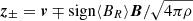 , in which BR is the radial component of the magnetic field and z± corresponds to outward and inward propagating fluctuations, respectively. With these variables, Alfvénicity is equivalent to z+ ≫ z−. We further defined the Elsasser energy, E± = 1/4⟨z±|2⟩, with ⟨…⟩ indicating a spatial or temporal average, and we used a hat for the power spectral density,
 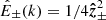 , with
  being the Fourier transform of z±.
On average, E+ decreases with distance faster than E−. This behavior is the opposite of what occurs in homogenous turbulence in which the energy of the subdominant species is damped more rapidly (dynamic alignment, Dobrowolny et al. 1980). Inside, 1 au E+ ∝ 1/R1.7, which is faster than what was expected from expansion (∝1/R) because of turbulent dissipation. The energy in z− follows a milder decrease, sometimes compatible with a constant energy or at worst decreasing as E− ∝ 1/R0.6 (Bavassano et al. 2002; Chen et al. 2020). The above scalings result from the development and evolution of turbulence with distance, which is not self-similar (e.g. Bavassano et al. 1982a,b; Denskat & Neubauer 1982; Horbury et al. 1996; Roberts 2010). Indeed, spectra are power laws whose indexes differ for magnetic and velocity fluctuations, changing with distance, latitude, and the type of solar wind stream (e.g. Bavassano et al. 2000, 2002; Horbury & Balogh 2001; Podesta et al. 2007; Salem et al. 2009; Chen et al. 2013, 2020; Wicks et al. 2013; Shi et al. 2021; Huang et al. 2023). Understanding the spectral evolution is hence required to explain the decay of energy with distance and the plasma heating.
Most of what we know on the spectral evolution of  inside 1 au comes from the analysis of three particular Alfvénic streams, often termed Bavassano and Bruno streams (B&B hereafter) owing to the authors who mostly analyzed them (their first analysis was given in Bavassano et al. 1982a; Denskat & Neubauer 1982). Such streams were detected by the Helios s/c at three heliocentric distances with a recurrence of about one solar rotation, since they were originating from the same large-scale coronal hole. In the following, for the sake of simplicity we shall use their properties as a reference for the evolution of turbulence and we shall return in Sect. 8 to the consequences of variations in spectral indexes and radial trends.
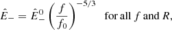
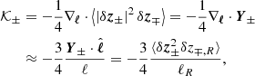
A schematic overview of the evolution of  is given in Fig. 1. The
  spectrum has a double power-law shape, with scaling roughly as f−1 and f−5/3 at small and large frequencies, respectively. The energy per unit mass per frequency band decays as 1/R at large scales and as 1/R2 at small scales (Bavassano et al. 1982b). The decay is not self-similar because the frequency break that divides the two ranges sweeps toward lower frequencies as fc ∼ 1/R3/2 (Bruno & Carbone 2013; Wu et al. 2021, 2020, 2022a), although in the distant heliosphere a slower scaling is observed, fc ∼ 1/R1.1 (Horbury et al. 1996). The nature of z− is less clear, and early observations show that at all heliocentric distances its spectrum has a power-law scaling with a Kolmogorov-like index, f−5/3. In addition, its energy does not decay, or decays very slowly, with distance, suggesting the existence of a background spectrum for z− (Tu & Marsch 1990). Now, it can be shown (see the next section) that the spectral evolution of
  can be explained if the spectral break results from the balance between the expansion timescale and a Kolmogorov-like cascade timescale, as was first proposed by Tu et al. (1984)2. Recovering the observed scaling of the frequency break requires the following assumptions: at large scales,
  , and it varies with distance as 1/R, while
  at all scales and its energy does not vary with distance within 1 au. These constraints are indicated as black lines and arrows in Fig. 1, while the grey color is used for properties that can be derived from them.
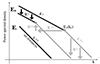 |
Fig. 1. Schematic view of the spectral evolution with distance of |


In this work, we use data from the WIND s/c at 1 au to compare expansion and turbulence losses, to verify if and how the balance between expansion and cascade occurs, and finally which of the above assumptions to recover the scaling of the frequency break are satisfied. The analysis of data exploits the Politano-Pouquet relation (von Karman & Howarth 1938; Politano & Pouquet 1998), which is able to quantify scale-dependent properties of turbulence: decay, cascade, and dissipation (cf. Hellinger et al. 2021). In addition, the effects of the expansion can be included via the expanding box model (EBM, Grappin et al. 1993). We use a form adapted to incompressible magnetohydrodynamics (MHD) that was derived in Hellinger et al. (2013). To summarize, we would like to answer the following questions: whether there is a separation of scales between turbulence and expansion; why  has a flat spectrum at large scales whose power spectral density decays as 1/R; and why the energy and power law scaling of
  do not vary with distance. While it is quite obvious that we cannot say anything about the origin of the 1/f spectrum at large scales using data at 1 au, our analysis will allow us to better understand the spectral properties of E± and to predict their decay with distance.
The structure of the paper is the following. Section 2 explains how the spectral evolution in Alfvénic streams can be understood by simple phenomenological arguments and a few observational constraints. In Sect. 3, we briefly comment on the Politano-Pouquet relation in the framework of the EBM; that is, a scale-to-scale energy budget equation in which the plasma expansion is accounted for. In Sect. 4, we describe the analyzed intervals of data and how we determine the terms entering the energy budget equation for each field, z±. Sections 5 and 6 contain the results of our analysis of the Politano-Pouquet relation applied to a non-Alfvénic and an Alfvénic stream, respectively. In the next two sections, we focus on the Alfvénic stream. In Sect. 7, we use results at 1 au to infer how the Elsasser energies decay with the distance. In Sect. 8, we compare the turbulent losses with the injection from sweeping of the frequency break and find an inconsistency in the energy budget of turbulent fluctuations. In the final section, we summarize the main results of our work, discuss their impact and limitation, and outline possible reasons for the above inconsistency.
2. Spectral evolution: Phenomenology
In the following, we assume that the Taylor hypothesis holds for the frequencies of interest, so that frequencies transform into wave numbers as f = kVSW, where VSW is the solar wind speed that is assumed to be much larger than the Alfvén speed, VSW ≫ VA. We now show how we can understand the spectral evolution of the solar wind turbulence starting from the following two observational constraints. (i) At large scales, the spectrum of z+ is flat and its energy varies as 1/R with distance; that is,
where  is the spectral energy density per unit mass evaluated at a given scale, f0, and a given distance, R0. (ii) The spectrum of z− has a unique power law with a Kolmogorov spectral index and it does not vary with distance; that is,
and again  is the spectral energy density per unit mass evaluated at a given scale, f0, at any distance.
Following Tu et al. (1984), we suppose that the frequency break is the scale at which the cascade timescale of z+ equals the timescale at which the plasma expands, tcasc+ = texp. We assume that the cascade timescale is the nonlinear timescale, and from Eq. (2) we have
^{-2/3}, \end{aligned} $$](/articles/aa/full_html/2024/10/aa50811-24/aa50811-24-eq21.gif)
where we have used the Taylor hypothesis, f = kVSW. The expansion timescale is defined as

where we have enforced a spherically expanding wind at a constant speed, VSW = const, oriented in the radial direction. Since the nonlinear timescale is independent of R and decreases with scale, while the expansion timescale increases with R and is independent of f, at any given distance there exists a scale, fc, for which the two timescales are equal. For f < fc the dynamics is dominated by expansion, while for f > fc the nonlinear dynamics dominates. By imposing the equality of timescales one obtains the critical wave number,
![$$ \begin{aligned} \frac{f_c}{f_0}=\left[\frac{2V_{\rm SW}/R_0}{z_-^0f_0/V_{\rm SW}}\right]^{3/2}\times \left(\frac{R}{R_0}\right)^{-3/2}, \end{aligned} $$](/articles/aa/full_html/2024/10/aa50811-24/aa50811-24-eq23.gif)
which corresponds to the observed scaling of the frequency break. In the square brackets we have the ratio of the nonlinear timescale over the expansion timescale evaluated at a reference scale, f0, and distance, R0. At a given distance, the break occurs at smaller scales for slower wind or for larger sunward fluctuations, independently of the value of  .
.
We finally derive how  decays with distance in the branch of the spectrum that is dominated by the cascade; that is, for f > fc. At those wave numbers,
  has a Kolmogorov slope; thus, the unique solution that also ensures a constant cascade rate for
  is again a Kolmogorov scaling,
where  is the spectral energy density evaluated at the scale of the break that varies with distance according to Eq. (5). To evaluate how
  changes with distance, we considered the following situation, which is illustrated schematically in Fig. 1. At large scales,
  is decreasing as 1/R, but at the same time the frequency break is climbing along the 1/f spectrum at a rate proportional to R−3/2; thus, the energy at the break at a new distance, R, must increase as
Substituting Eqs. (7) and (5) into Eq. (6) we finally obtain
which gives the observed scaling with distance (Bavassano et al. 1982a). We stress that the faster 1/R2 decay follows from the decay of energy in the 1/f part of the spectrum and from the sweeping of the frequency break. In fact, in the inertial range the energy is transferred toward smaller scales without dissipation. In this framework, the injection of energy in the turbulent cascade is due to the shift of the frequency break. We can thus evaluate the loss of energy associated with the variation in “width” of the low-frequency branch as the product of the spectral energy density at the break times the variation in the break scale:
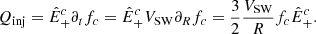
In the second equality we assumed that the plasma is moving at a constant solar wind speed and for the third equality we used the scaling of the break with distance, Eq. (5), which brings the coefficient 3/2 in front of the expression: the faster the break sweeps, the stronger the energy injection is. When the Alfvén speed is much smaller than the solar wind speed, this expression is equivalent to the one obtained from the spectral model of Tu et al. (1984) and compared to the perpendicular heating rate of protons in Wu et al. (2020, 2021, 2022b). In this work, we instead estimate the proton heating rate as the one required to maintain a nonadiabatic temperature decrease, Tp ∝ R−γ, obtained from the evolution of temperature of a plasma parcel that is advected at a constant radial solar wind speed (Verma et al. 1995; Vasquez et al. 2007),
Since we are using measurements at 1 au only, we use γ = 1 ± 0.2 as a power-law index for the temperature decrease (Totten et al. 1995; Hellinger et al. 2013; Maksimovic et al. 2020).
3. Expanding box model and the Politano-Pouquet law
Following Hellinger et al. (2013), we outline a derivation of the Politano-Pouquet law including expansion terms (more details can be found in that paper, but see Gogoberidze et al. 2013 for a different approach and final equation). We started from the EBM originally derived for fully compressible MHD (Grappin & Velli 1996). We recall that EBM describes the evolution of a parcel of plasma moving radially from the sun at a constant speed higher than the Alfvén velocity. Expansion provides two main effects: it stretches the volume in the coordinates perpendicular to the radial direction, introducing anisotropies in the field gradients; and it introduces linear damping terms proportional to the expansion rate so that linear invariants are preserved (energy is not conserved because of the work done by the expansion on the plasma volume). Thus, EBM takes into account the volume expansion, while ensuring the conservation of mass, momentum, magnetic flux, and adiabatic evolution in the absence of external heating and/or heat fluxes. We first obtained the incompressible MHD equations in the EBM by imposing incompressibility in the induction and momentum equations (no continuity and pressure equations were needed). Then, we rewrote the equations of incompressible MHD in term of the Elsasser fields by dividing the induction equation with the average density and summing and subtracting it from the momentum equation. Assuming equal resistivity and viscosity, η = ν = μ/ρ, one obtains
![$$ \begin{aligned} \partial _t\boldsymbol{z}_{\pm }+\boldsymbol{z}_{\mp } \cdot \mathbf{\nabla }\boldsymbol{z}_{\pm }-\nu \mathbf{\nabla }^2 \boldsymbol{z}_{\pm }+\mathbf{\nabla } P_{\rm tot}=-\frac{1}{2} \frac{V_{\rm SW}}{R}\left[\boldsymbol{z}_{+} +\boldsymbol{z}_{-} -2\boldsymbol{z}_{{\mp ,R}}\right], \end{aligned} $$](/articles/aa/full_html/2024/10/aa50811-24/aa50811-24-eq36.gif)
where on the right-hand side we have grouped the new terms related to expansion and the index R indicates the radial component of fluctuations of the Elsasser variables. This form explicitly shows that expansion introduces non-diagonal terms that couple z± via the inhomogeneity of the flow, ∇ ⋅ VSW = VSW/2R; that is, a reflection term in a particularly simple form.
Apart from the new linear terms on the right-hand side, the equations are formally identical to those of the incompressible MHD. Following the same procedure as the homogenous case (e.g. Politano et al. 1998; Carbone et al. 2009), one obtains the usual Politano-Pouquet law plus some terms proportional to the second-order structure functions and the expansion rate. Specifically, we evaluated Eq. (11) at a position, x, and x + ℓ, with ℓ being a vector increment, took the difference between them, and multiplied them by the increments δz± = z±(x + ℓ)−z±(x). After averaging over space, ⟨…⟩, and exploiting the assumptions of homogeneity and incompressibility, the Politano-Pouquet law reads:
![$$ \begin{aligned} \frac{1}{4}\partial _t \left\langle \left| \delta \boldsymbol{z}\pm \right|^2 \right\rangle =&-\epsilon _\pm + \frac{1}{2}\nu \mathbf{\nabla }_\ell ^2\left\langle \left| \delta \boldsymbol{z}\pm \right|^2 \right\rangle \\&-\frac{1}{4}\mathbf{\nabla }_\ell \cdot \left\langle \left| \delta \boldsymbol{z}_{\pm } \right|^2\delta \boldsymbol{z}_{\mp } \right\rangle \nonumber \\&-\frac{1}{4}\frac{V_{\rm SW}}{R}\left[\left\langle \left| \delta \boldsymbol{z}\pm \right|^2 +\delta \boldsymbol{z}_{+}\cdot \delta \boldsymbol{z}_{-} -2\delta \boldsymbol{z}_{+,R}\cdot \delta \boldsymbol{z}_{-,R} \right\rangle \right]\nonumber . \end{aligned} $$](/articles/aa/full_html/2024/10/aa50811-24/aa50811-24-eq37.gif)
On the right-hand side, ϵ± = ⟨ν∂izj±∂jzi±⟩= − 2dtE± is twice the dissipation rates of the two Elsasser energies (E± = ⟨z±2⟩/4), ν is the viscosity, also equal to the resistivity, and gradients have been computed with respect to the increment, ℓ. In the last term, R is the radial distance, VSW is the (constant and radial) solar wind speed, and the index R indicates the radial component of z±. All quantities, except ϵ±, are functions of the increment, ℓ, and Eq. (12) is a scale-to-scale energy budget equation. We recall that on the left-hand side, the time derivative represents the variation with radial distance. In fact, it is taken in the frame of the expanding box that is moving at a constant speed in the radial direction, from which ∂t = VSW∂R.
We next proceeded by assuming isotropy, since spectral anisotropy cannot be computed from single s/c data and would require further assumptions on the geometry of turbulence. Isotropy allows us to consider increments as scales and to give a simple interpretation of each term (a similar meaning can be obtained by integrating on a sphere and by using Gauss’ theorem, as in Wang et al. 2022). We thus define
which is the energy density of z± fluctuations at scales ≤ℓ,
which is the dissipation of energy at scales < ℓ,
which is the energy flux coming from scales larger than ℓ, and finally
![$$ \begin{aligned} {\mathcal{F} }^{\exp }_\pm = -\frac{V_{\rm SW}}{R}\left[{\mathcal{S} }_\pm +{\mathcal{S} }_R\right], \end{aligned} $$](/articles/aa/full_html/2024/10/aa50811-24/aa50811-24-eq41.gif)
which is the forcing (often a damping, as we shall see) due to expansion acting on scales ≤ℓ. Using the above definitions, the scale-to-scale energy budget equation has a compact form,
with the following meaning. The variation with distance of the energy density of fluctuations at scales smaller than ℓ is due to the competition between the supply of energy coming from scales larger than ℓ (𝒦) and the damping of energy at scales smaller than ℓ, which is realized by turbulent dissipation (−𝒟) and expansion (ℱexp).
A few comments are in order. First, in Eq. (15) we have implicitly defined the third-order mixed structure functions (i.e., a vector field), often termed the Yaglom field, as Y± = ⟨δz±2δz∓⟩. Obtaining the cascade rate requires computing the divergence of Y± in the increment space, which is clearly not feasible with single s/c data (Pecora et al. 2023a). Our estimate of the cascade rate, 𝒦, is based on the assumption of isotropy that allows us to write the second-last equality in Eq. (15) (see e.g., Stawarz et al. 2009 for anisotropic versions that are based on heuristic geometric models of turbulence). There  indicates the projection of the Yaglom field in the direction of increments, and in the next equality we used the index R to specify that both Y and ℓ are necessarily along the solar wind radial flow. When 𝒦 takes a constant positive value within a range of scales, we can identify this range as an inertial range: in fact, for any given scale, ℓ, belonging to this range the energy flux coming from scales > ℓ is the same; in other words, the cascade of energy is constant in this range. If, instead, 𝒦 has a negative constant value within a range of scales, we can interpret it as a range in which an inverse cascade is occurring. However, since 𝒦 is a signed quantity, it requires a large statistic to converge (see for example Podesta et al. 2009), and positive and negative constant values are almost equally probable on a scale of about an hour (Coburn et al. 2014). Second, in writing the expansion term, Eq. (16), we implicitly defined the second-order structure function for the (component-anisotropic) residual energy,
At variance with the cascade rate, only the use of EBM is required to obtain ℱ±exp from single s/c data, and since it involves only second-order structure functions its calculation rapidly converges. ℱ±exp has two contributions: a diagonal term proportional to the field, 𝒮±, which is responsible for the so-called WKB losses and leads to an energy decay ∝1/R; and a non-diagonal term (i.e., involving the product of δz+ and δz−) that we label Non-WKB, since it may cause deviation from the 1/R decay by coupling the two energies, 𝒮±, via the background inhomogeneity and since it is non-vanishing when |δv|≠|δb|.
It is instructive to examine the energy budget, Eq. (17), written for the total energy to highlight the contributions of each term on different scales. Since the total dissipation is ϵ = (ϵ+ + ϵ−)/2, the energy budget equation is formally the same (just neglect the subscripts ±) if we use the following definitions: 𝒮 = (𝒮+ + 𝒮−)/2, 𝒟 = (𝒟+ + 𝒟−)/2, 𝒦 = (𝒦+ + 𝒦−)/2, and
![$$ \begin{aligned} {\mathcal{F} }^{\exp }=({\mathcal{F} }^{\exp }_++{\mathcal{F} }^{\exp }_-)/2&=-\frac{V_{\rm SW}}{R}[{\mathcal{S} }+{\mathcal{S} }_R]\\&=-\frac{1}{2}\frac{V_{\rm SW}}{R}[\langle \delta \boldsymbol{v}_\bot ^2\rangle +\langle \delta \boldsymbol{b}_R^2\rangle ].\nonumber \end{aligned} $$](/articles/aa/full_html/2024/10/aa50811-24/aa50811-24-eq45.gif)
The latter expression shows that expansion is always a damping term for the total energy, although only proportional to part of it. At large scales (LS), the cascade is negligible while 𝒟 = ϵ, the structure function is twice the total energy, and one can finally write

that is, the damping of energy is given by the sum of the turbulent damping and expansion damping. While the left-hand side of Eq. (20) cannot be computed with single s/c data (we recall that ∂t ≡ VSW∂R), we can directly evaluate ℱexp on the right-hand side and indirectly evaluate the turbulent dissipation by considering the total energy budget, Eq. (17), in the inertial range (IR). There, ℱexp is negligible since it is proportional to 𝒮 and 𝒮R, which are decreasing functions of scale. In a quasi-stationary state the energy is conserved in the inertial range; the left-hand side vanishes, so that one has

which allows one to compute the turbulent dissipation, ϵ. The flux coming from scales larger than ℓ is balanced by the total dissipation at scales smaller than ℓ. Thus, although we cannot directly measure the damping of energy with distance, we estimated it by obtaining the turbulent damping and the damping due to expansion at inertial and large scales, respectively.
One can obtain a similar equation for the cross helicity, 𝒮c = (𝒮+ − 𝒮−)/2, with analogous definitions of the other terms, 𝒦c = (𝒦+ − 𝒦−)/2, ϵc = (ϵ+ − ϵ−)/2, and
If the cross helicity also decreases with scale, a separation of scales should hold, similar to that for the total energy. In Sect. 7, we evaluate at 1 au the energy budget Eqs. (20), (21) for E±. We also find constraints that allow power-law scaling for the decay of energies with distance, and thus the extrapolation of E± in the inner heliosphere.
4. Data interval and analysis
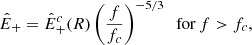
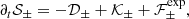
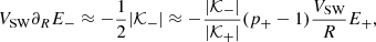
We have used data collected on the WIND s/c by 3DP/PESA-LOW and MFI instruments, the latter resampled at a 3 s resolution on proton data, during the year 1995 from DOY 126 at 0 h to DOY 131 at 12 h, a period previously studied in D’Amicis et al. (2019) to distinguish properties of fast and slow Alfvénic streams, compared to traditional slow streams. An overview of the data is given in Fig. 2, with green-shaded areas highlighting the two intervals that are analyzed in the following. From top to bottom, with black lines, we plot the solar wind speed, VSW, the proton temperature, T, and the correlation between the velocity and magnetic fluctuations, CvB = Δv ⋅ ΔB/|Δv||ΔB|, where Δv = v − ⟨v⟩1 h is the velocity fluctuation obtained by subtracting a running average on a 1 h scale (and similarly for the magnetic field, B). The shaded light green area corresponds to a fast and hot stream, with a strong correlation between fluctuations; in other words, a strongly Alfvénic stream. The shaded dark green area corresponds to a slow and cold stream with poor correlation; in other words, a non-Alfvénic stream (these intervals roughly correspond to 3F and 3TS, respectively, in Table 1 of D’Amicis et al. 2019). With red lines in the top and middle panels, we also plot the magnetic field intensity (|B|) and the proton density (n), respectively. The two intervals were selected because both |B| and VSW are roughly constant. However, in the slow stream, n increases linearly. Our analysis is based on incompressible MHD, and thus this trend impacts the average n0 used to define magnetic fluctuation in Alfvén units. In the fast stream, one can see that fluctuations on a scale of about half a day are approximately correlated in VSW and T, as well as in n and |B|; also, VSW is approximately anticorrelated with n (and so T with |B|). This suggests that the fast stream interval has a substructure of jets that are faster, hotter, fainter, and less magnetized, possibly representing patches of switchback trains. For completeness, the main average properties of the two streams are summarized in Table 1.
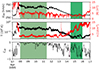 |
Fig. 2. Overview of the selected intervals of fast and slow streams. Light green and green areas correspond to the fast Alfvénic and slow non-Alfvénic streams, respectively. From top to bottom: Solar wind speed, VSW (black), and magnetic field intensity, |B| (red); proton temperature, T (black), and proton density, n (red); correlation between magnetic and velocity fluctuations, CvB, at a 1 h scale. |
Main characteristics of the non-Alfvénic (NALF) and Alfvénic (ALF) streams.
Within each interval, we computed time increments, τ, of the velocity and magnetic fields, δv = v(t + τ)−v(t) and δb = b(t + τ)−b(t), where  , with n0 being the average density (mp and μ0 are the proton mass and the vacuum permittivity). Finally, we obtained time increments of the Elsasser fields from those of velocity and magnetic fluctuations as δz± = δv ∓ sign⟨BR⟩δb, where ⟨BR⟩ is the average radial magnetic field components. In this way, z± indicate outward and inward propagating fluctuations independently of the direction of the mean magnetic field. We finally constructed second- and third-order structure functions, 𝒮±, 𝒮u, 𝒮b, 𝒮R, by averaging over t. We could now obtain the cascade rates, 𝒦±, in Eq. (15) and the expansion terms, ℱ±exp, in Eq. (16) by using the s/c position (R = 1 au for the WIND s/c) and the Taylor hypothesis to convert time increments into space increments in the (only accessible) radial direction, ℓ = ⟨VSW⟩τ, with ⟨VSW⟩ the average solar wind speed.
We now show the results of applying the Politano-Pouquet law to the non-Alfvénic stream and we consider the Alfvénic stream in the next section. Often log-log plots will be used to show second- and third-order structure functions that may have a positive or negative sign. As a rule, we plot the absolute values of any quantity, using thick lines when it is positive and thin lines when it is negative.
5. Slow non-Alfvénic stream
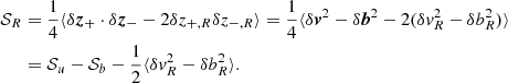
The second-order structure function, 𝒮±, computed in the non-Alfvénic stream is shown in Fig. 3 with black and red lines, respectively. As was expected for a low-cross-helicity stream, the two structure functions coincide at all scales, with the exception of the very large ones (τ ≳ 3 h). On small scales, τ ≲ 0.1 h, a Kolmogorov-type scaling is clearly visible, with 𝒮 ∝ ℓ2/3 (dotted line), while at intermediate scales, 0.1 h ≲ τ ≲ 3 h, the structure function is flatter. In the same plot, the component-anisotropic residual energy, 𝒮R, is also shown with a blue line: it is negative at all scales but its value is a factor of three smaller than 𝒮± and somehow smaller at small scales. This implies that the expansion term, ℱ±exp, is dominated by 𝒮± and is a damping term (see Eq. (16)).
 |
Fig. 3. Second-order structure functions for the two Elsasser fields, 𝒮+ and 𝒮−, in black and red lines, respectively, for the non-Alfvénic interval. The component-anisotropic residual energy, 𝒮R in Eq. (18), is plotted in blue. A thin line is used for negative values and a thick line for positive ones. The dotted line is a reference for the Kolmogorov scaling, 𝒮 ∝ ℓ2/3. |
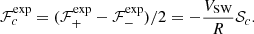
We now show in Fig. 4 the cascade rate, 𝒦±, and the expansion rate, ℱ±exp, with green and blue lines, respectively, for z+ (top panel) and for z− (bottom panel). Considering first the cascade rate in green lines: while 𝒦+ in the top panel is more irregular and changes sign every decade in scales, 𝒦− in the bottom panel has a flat part in the range of 0.05 h ≲ τ ≲ 3 h, indicating the presence of a constant cascade rate in an extended inertial range. This qualitative difference also impacts the value of the cascade, with 𝒦− ≈ 5𝒦+, and is in contrast with the similarities of 𝒮±. However, since this interval has relatively strong fluctuations in density, along with an increase in its average value, it is surprising that the isotropic incompressible approximation of the Politano-Pouqet law works quite well, at least for one species. Considering now the expansion terms, ℱ±exp (blue lines), which are basically identical because of the similarities in 𝒮±: expansion is negative (thin line); that is, it is a damping term whose importance decreases with scale. For z−, it is comparable to the cascade rate at large scales, τ ≳ 3 h, with an average value of ≈600 W/kg for scales larger than a few hours, and it becomes negligible for τ ≲ 1 h (for z+, it becomes negligible at smaller scales, τ ≲ 0.1 h). We can somehow identify the beginning of the inertial range with the scale at which the cascade becomes constant: τ ≈ 2 h. When the damping due to expansion is comparable to the turbulent damping evaluated at inertial range scales, energy starts to be efficiently transferred to smaller scales; in other words, we are entering the injection range at a scale of τ ≈ 6 h. Thus, comparing expansion and turbulent damping and examining the form of 𝒦(τ), the injection range for the non-Alfvénic stream can be identified with the scales τ ∈ [2, 6] h, while expansion perhaps becomes important at larger scales.
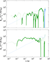 |
Fig. 4. Cascade rate and expansion losses, 𝒦 and ℱexp, respectively, in green and blue lines, for the Elsasser field z+ and z− (top and bottom respectively) in the non-Alfvénic stream. Thick (thin) lines indicate positive (negative) values. |
Until now, we have analyzed the energy budget equation of the Elsasser energies, 𝒮±. An alternative but equivalent viewpoint is offered by an inspection of the total energy and of the cross helicity, whose cascade and expansion are plotted in Fig. 5. The total energy in the left panel does not show much difference compared to 𝒮− in Fig. 4, but we can see that on small scales the total losses change sign and are smaller. This is a consequence of 𝒦± having the opposite sign and similar values on small scales. The cross helicity in the right panel has an interesting aspect: the expansion term is negligible at inertial range scales, while it is a source and comparable to the cascade at large scales. However, interpreting non-Alfvénic turbulence with incompressible MHD may be misleading and a fully compressible analysis is required (see Montagud-Camps et al. 2022 for an application to MHD simulations).
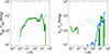 |
Fig. 5. Cascade and expansion losses for the total energy (left) and the cross helicity (right) for the non-Alfvénic stream. |
6. Fast Alfvénic stream
In Fig. 6, we show the second-order structure functions for the Alfvénic stream: as was expected, 𝒮+ ≫ 𝒮− at all scales (compare the black and red lines) but their spectral properties differ. At large scales, τ ≳ 3 h, 𝒮+ is flat and reflects the presence of the 1/f range in the power spectrum. At intermediate scales, no clear power-law scaling is seen, and finally at small scales, τ ≲ 0.1 h, a Kolmogorov-like scaling shows up. On the contrary, 𝒮− has a unique power-law scaling for 0.01 h ≲ τ ≲ 10 h with a relatively flat spectrum that approximately follows 𝒮− ∝ ℓ0.4. At very small scales, 𝒮− flattens, possibly because of the noise in the velocity measurements. In the same figure, we plot with a blue line the (component-anisotropic) residual energy, 𝒮R, which is again negative. Its value is much smaller than 𝒮+, meaning that the latter determines the shape of the expansion term, ℱ+exp. On the contrary, the absolute value of 𝒮R is comparable to and even slightly larger than 𝒮−, and its expansion term will substantially differ from the non-Alfvénic case, as we see below.
The cascade and expansion terms for z± are plotted in the top and bottom panels of Fig. 7, respectively, with the same format of Fig. 4 (green and blue lines for 𝒦 and ℱexp, respectively, and thin and thick lines for negative and positive values, respectively). As in the previous case, ℱ+exp < 0, expansion is a damping term for the dominant Elsasser field and its shape follows the one of 𝒮+. In the 1/f part of the spectrum, the only damping is due to expansion, and because 𝒮+ ≫ |𝒮R| it implies a WKB scaling. The energy per unit mass per frequency band is expected to decay as 1/R. The cascade, 𝒦+, is negligible (and negative) at large scales belonging to the 1/f range, τ ≳ 3 h, then its value slowly increases and finally reaches a constant (positive) value for a decade at scales of 0.01 h ≲ τ ≲ 0.1 h that we identify as the inertial range. The inertial range is established at smaller scales with respect to the non-Alfvénic case.
The separation of scales between 𝒦+ and ℱ+exp supports the original idea of Tu et al. (1984) that the large-scale break in the frequency spectrum marks the separation between scales whose dynamics is governed by the turbulent cascade or by expansion. In addition, the rough equality between the damping due to expansion at large scales and turbulence at small scales (𝒦+ ≈ ℱ+exp ≈ 1.2 × 10⁴ W/kg) suggests that in a stationary state the position of the frequency break adapts – shifts to lower frequencies – in order to maintain a balance between the expansion time and the cascade time. As in the non-Alfvénic stream, we can identify the injection range with τ ∈ [0.1, 3] h, where the small scale is the top of the inertial range and the large scale is identified with the scale at which the damping due to expansion is comparable with the turbulent damping measured at inertial range scales. The injection range is larger than in the non-Alfvénic stream because the cascade develops at a smaller scale, while injection starts at about the same large scales. The large scale is placed where ℱ+exp starts to decrease and coincides with the scale at which also 𝒮+ starts to decrease; a plausible location of the frequency break at the end of the 1/f range.
Considering now the cascade and expansion for z− in the bottom panel of Fig. 7: at large scales, τ ≳ 3 h, the expansion terms oscillates and its absolute value is negligible. In fact, as was anticipated when analyzing second-order structure functions, ℱ−exp ≈ 0 because 𝒮− and 𝒮R compensate each other. Also, the cascade rate is small and of the same order, so that at large scales z− is not damped. At first sight, this is consistent with the existence of the background spectrum of  , as was suggested by Tu & Marsch (1990). At intermediate scales, the expansion term is constant and positive, meaning that ℱ−exp is a source of energy for the subdominant species. In the same range, the cascade rate increases, then it changes sign while keeping the same absolute value, and stays constant for a decade. Neglecting the change of sign, the inertial range of z− begins at larger scales, τ ≈ 1 h. Although acting on about a decade in scale, and thus possibly changing the nature of nonlinear interactions with respect to the homogenous case, the expansion is ten times smaller than the absolute value of the cascade. Thus, we expect E− to not keep the same energy with distance but to be weakly damped by the cascade.
Comparing the top and bottom panels of Fig. 7, it is evident how the third-order structure functions, 𝒦±, have opposite signs in the whole range of scales at which the cascade is somehow regular for both species (τ ≲ 3 h). Additionally, each of them changes sign at a scale of about 0.2 h. The physical origin for the opposite sign of 𝒦± can be understood by recalling that even in Alfvénic streams a magnetic energy excess develops. Since 𝒦± ∝ ⟨|δz±2|δz∓, R⟩, the sign of the proxy for the cascade is given by that of δz∓, R, weighted by the energy of fluctuations, |δz±2|. If large fluctuations are correlated with a strong magnetic excess, δb ≫ δu, then 𝒦± have opposite signs (see also Coburn et al. 2015; Vasquez et al. 2018, for details). The switch of sign at a given scale is probably due to a change in the symmetry of fluctuations around zero at that scale (e.g., from positive to negative skewness), but its physical origin has not been investigated yet. We speculate that expansion may play a role, since it introduces correlations thanks to the residual energy term, 𝒮R ∝ ⟨δz+ ⋅ δz−⟩, and acts on the same scale at which the switch of sign is observed. Both phenomena are reported in many works (Sorriso-Valvo et al. 2007; Stawarz et al. 2010, 2011; Coburn et al. 2014, 2015; Vasquez et al. 2018) and an attempt at classifying shapes of third-order structure function and how their occurrence varies with the type of stream in the Helios data is reported in Wu et al. (2022a). Concerning the energy budget of fluctuations, irrespective of the sign we consider |𝒦±| to be a good measure of the direct cascade of energy.
The profiles of 𝒮 and 𝒮c are shown for completeness in Fig. 8 and are very similar to those of 𝒮+ in Fig. 7. This is not surprising because 𝒮+ ≫ 𝒮−, |𝒦+|≫|𝒦−|, and |ℱ+exp|≫|ℱ−exp|. We remark that expansion damps cross-helicity not only at the largest scales as one may expect, but also on a wide range of intermediate scales.
7. Approximate decay of energy in Alfvénic stream
We summarize in Table 2, the values of the damping due to expansion, ℱ±exp, and due to the turbulent cascade, 𝒦±. The values were obtained by fitting the logarithm of the corresponding quantities to a straight line over a decade of scales and the uncertainties are the standard deviations in these intervals. Different fitting ranges have been used for the value 𝒦 in each stream; namely, τ ∈ [10−1, 1] h and τ ∈ [10−2, 10−1] h for the non-Alfvénic and Alfvénic streams, respectively, corresponding to one decade below the bottom of the injection range. The fitting ranges of ℱexp were obtained taking one decade above the injection range in the Alfvénic stream, while for the shorter non-Alfvénic stream we took the average for scales, τ ≥ 2 h.
Elsasser energy losses in the non-Alfvénic (NALF) and Alfvénic (ALF) stream.
We now seek solutions for the decay with distance of the Elsasser energies that satisfy the power-law scaling, E± ∝ R−p±. After having identified the relevant terms in the energy budget equation on large scales, Eq. (20) for 𝒮±, we used simple assumptions to extrapolate them at smaller distances. Although the cascades, 𝒦±, have opposite signs, in the following we consider their absolute value to be a measure of a direct cascade of energy.
In the previous section, we found that 𝒮+ is damped by expansion at large scales, while at small scales turbulent damping takes over with a value close to the large-scale expansion losses, |ℱ+exp|≈𝒦+ in Table 2. Thus, E+ is damped by both expansion and turbulence, and the energy budget equations at large scales, Eq. (20), can be written as
![$$ \begin{aligned} V_{\rm SW}\partial _RE_+\approx -\frac{1}{2}\left(|{\mathcal{K} }_+|+|{\mathcal{F} }^{\exp }_+|\right) =-\left[1+\frac{|{\mathcal{K} }_+|}{|{\mathcal{F} }^{\exp }_+|}\right]\frac{V_{\rm SW}}{R}E_+, \end{aligned} $$](/articles/aa/full_html/2024/10/aa50811-24/aa50811-24-eq51.gif)
where we have used E+ = 𝒮+|LS/2 and ℱ+exp/2 = −(VSW/R)E+. The assumption of 𝒦+/ℱ+exp = const at all distances yields a power law decrease for E+ with
![$$ \begin{aligned} p_+=\left[1+\frac{|{\mathcal{K} }_+|}{|{\mathcal{F} }^{\exp }_+|}\right]\approx 2, \end{aligned} $$](/articles/aa/full_html/2024/10/aa50811-24/aa50811-24-eq52.gif)
where in the last approximation we used |𝒦+|/|ℱ+exp|≈1, evaluated at 1 au in Table 2. E+ decays faster than WKB because of the turbulent dissipation, as fast as R−2.
We consider now the subdominant field, for which we found that 𝒮− has negligible damping at large scales (ℱ−exp ≈ 0 in Table 2), while at intermediate and small scales expansion is a source of energy but much smaller than the cascade. Ultimately, 𝒮− should be damped by the cascade with ϵ− ≈ 𝒦−. We first write its energy budget equation as
where we have used E− = 𝒮−|LS/2 and |𝒦+|=(p+ − 1)|ℱ+exp| from Eq. (24). A power-law solution, E ∝ R−p−, is found by assuming that the ratio of the energy cascades does not vary with distance, 𝒦−/𝒦+ = const. Inserting E+ ∝ R−p+, we obtain p− = p+. E− should scale as E+. However, this solution is inconsistent with our data at 1 au, which instead yield p− < p+. To see this, one should first consider again Eq. (25) and multiply the right-hand side by E−/E− to obtain
\frac{V_{\rm SW}}{R}E_-. \end{aligned} $$](/articles/aa/full_html/2024/10/aa50811-24/aa50811-24-eq54.gif)
Since E± have the same scaling, the term in square brackets is constant and yields for a power-law index of E−,
\approx 1.1, \end{aligned} $$](/articles/aa/full_html/2024/10/aa50811-24/aa50811-24-eq55.gif)
where in the last approximation, we used E+/E− ≈ 6 and |𝒦+|/|𝒦−|≈5.5, evaluated at 1 au in Tables 1 and 2, respectively, along with p+ ≈ 2.
Different scaling laws for E± can be obtained by imposing a constant ratio of the cascade rates of the two species (the term in square brackets), which implies the same scaling for the ratio of cascades and energies, 𝒦−/𝒦+ ∝ E−/E+ ∝ Rκ, with
\approx 0.9, \end{aligned} $$](/articles/aa/full_html/2024/10/aa50811-24/aa50811-24-eq56.gif)
and again we used data at 1 au in the last approximation.
To summarize, we obtained power-law solutions of E± by assuming invariance with distance of the ratio of the cascade over expansion losses of E+ and of the ratio between the cascade rates of the two species. This implies that E− decays more slowly than E+ and the difference between their power-law indexes is equal the power-law index, κ, characterizing the increase with distance of the ratio of their energy cascades. Using the values from our analysis at 1 au (see Tables 1 and 2) we obtain E+ ∝ R−2, E− ∝ R−1.1, and 𝒦−/𝒦+ ∝ R0.9.
8. Cascade of total energy versus heating and injection
We now analyze more quantitatively the differences between non-Alfvénic and Alfvénic streams, by showing in Table 3 for the total energy the values of the damping due to expansion, ℱexp, and due to the turbulent cascade, 𝒦, along with the injection range (first column) that we identified in the previous section. Values and errors for 𝒦 and ℱexp were obtained, as before, by averages and standard deviations in the inertial range (τIR) and in a range approximately above the injection range (τinj), respectively. For both streams, we find that expansion damping is slightly larger than the cascade. The value of 𝒦 is about 15 times larger in the Alfvénic stream that also has amplitudes about three times larger, suggesting that Alfvénicity leads to less efficient nonlinear interactions. We shall come back to such an evaluation at the end of the section, when we shall compare 𝒦 to phenomenological estimates. Anyhow, for both streams the energy cascade is compatible with the heating required to maintain a nonadiabatic decrease in the proton temperature, 𝒦 ≈ QVV. The latter was obtained by inserting into Eq. (10) the measured temperature at 1 au and assuming a power-law index of γ = 1 ± 0.2 for the temperature decrease.
Total energy losses and phenomenological estimates in the non-Alfvénic (NALF) and Alfvénic (ALF) streams.
We now focus on Alfvénic stream and compare the turbulent damping with the energy injected into turbulence by the sweeping of the frequency break toward larger scales, Qinj. The method of estimating it is illustrated in the Appendix A and requires identifying the frequency break, fc, in the power spectral density,  , and evaluating fcE+(fc), which enters Eq. (9). The estimated value is indicated in Table 3 and reveals that the injection from sweeping is three times smaller then the energy cascade, 𝒦, in the Alfvénic stream. A factor of three could be considered acceptable as an order of magnitude estimate of the balance between injection and dissipation. However, this factor should not be neglected for two reasons. First, it increases to six when comparing cascade and injection just for z+. Second, as we shall see below, the estimated value of energy injection is an upper limit, since it is obtained with the fastest possible scaling, fc ∝ R−3/2.
This fast scaling requires the following assumptions to hold: (i) turbulence must be strong for  so that the cascade time is the eddy-turnover time; (ii)
  should have an approximate Kolmogorov scaling (K41); and (iii) the energy of the subdominant species should not decay with distance (see Sect. 2 and Fig. 1). We have seen in Sect. 7 that instead E− must decrease with distance, while from Fig. 6 we get SF− ∝ ℓ1/2, suggesting an Iroshnikov-Kraichnan scaling, z− ∝ k−1/4 (Iroshnikov 1964; Kraichnan 1971). We can evaluate the cascade time by comparing 𝒦+ with K41 and IK phenomenologies built on second-order structure functions,
In front of the phenomenologies, α ≈ 0.1 is a reduction factor due to factorization of the third-order structure function into second-order structure functions (Vasquez et al. 2007; Bandyopadhyay et al. 2018; Montagud-Camps et al. 2018; Verdini et al. 2019). In Fig. 9, we plot 𝒦+ with green lines, QK41 with a thin grey line, and QIK with a thick grey line. Clearly, the IK phenomenology better reproduces both qualitatively and quantitatively the profile of 𝒦+, having a plateau in the inertial range, while the Kolmogorov phenomenology increases at inertial range scales. For completeness, in the last three columns of Table 3, we evaluate the K41 and IK phenomenology for the total energy at the beginning of the inertial range. Again, the IK phenomenology is close to the measured cascade, which is also in the non-Alfvénic stream, while K41 largely overestimates the cascade in both cases. This suggests that Alfvénicty does not reduce the efficiency of nonlinear interactions, contrary to expectations.
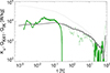 |
Fig. 9. Comparison between the measure cascade, 𝒦+, in the Alfvénic stream and two phenomenologies obtained using second-order structure functions: the Kolmogorov one plotted with a thin grey line and the Iroshnikov-Kraichnan one plotted with a thick grey line, Eqs. (29) and (30), respectively. |
Ultimately, none of the above assumptions hold, and we can instead use an IK timescale for the cascade rate, 1/t+casc = kz−z+/VA, a decay with distance, E− ∝ R−p−, and also an IK scaling, z− ∝ k−1/4, for its spectrum. For simplicity, we have kept VA = const,  at large scales and with a 1/k scaling. Imposing an equal expansion and cascade rate, 1/texp = 1/t+casc, one again obtains the break position and its scaling:
![$$ \begin{aligned} \frac{f_c}{f_0}=\left[\frac{2V_{\rm SW}/R_0}{f_0z_-^0z_+^0/V_{\rm SW}V_{\rm A}}\right]^{4/3}\times \left(\frac{R}{R_0}\right)^{-2/3(1-p_-)}, \end{aligned} $$](/articles/aa/full_html/2024/10/aa50811-24/aa50811-24-eq66.gif)
which clearly shows that the break moves at larger scales with distance but at a slower rate. No shift should be observed if p− = 1, while fc ∝ R−1/3 or fc ∝ R−2/3 if p− = 0.5 or 0, corresponding, respectively, to a slow decrease or no decrease (the latter being equivalent to the case of Sect. 2, but with an IK cascade). A slower shift of fc corresponds to less injection, and so the value of Qinj is an upper limit for the injection of energy.
We conclude that there is a potential inconsistency in the energy budget of turbulence for the Alfvénic stream: the injection of energy into turbulence by the sweeping of the frequency break is unable to sustain the cascade.
9. Discussion and conclusions
We have used velocity and magnetic time series from the WIND s/c at 1 au to understand at which scales the damping of fluctuations is dominated by expansion or by turbulence, with only the latter resulting in plasma heating. Both forms of damping were evaluated in the framework of the Politano-Pouquet relation (Politano & Pouquet 1998), a scale-to-scale energy budget equation for turbulent fluctuations in incompressible MHD. Turbulent damping was computed via third-order structure functions, assuming homogeneity, isotropy, and stationarity in the inertial range. Expansion damping was computed via second-order structure functions by implementing the EBM (Grappin & Velli 1996) in the Politano-Pouquet law for incompressible MHD (see Sect. 3 and Hellinger et al. 2013 for details). We analyzed first a non-Alfvénic stream, characterized by a low level of correlation between v and B, or, equivalently by similar amplitudes of the Elsasser variables, z+ ≈ z−. Then, we focused on an Alfvénic stream, with strong correlations between magnetic and velocity fluctuations, or equivalently z+ ≫ z−.
In the non-Alfvénic stream, the cascade and expansion of each Elsasser field have properties that are roughly similar to each other and to those of the total energy. Expansion is a damping term for E± and is negligible at scales below 2 h, where the cascade dominates. The transition is quite sharp, indicating a small injection range. In the Alfvénic stream, only E+ and the total energy have similar properties: expansion dominates over the cascade at large scales, while the cascade dominates over expansion at small scales. A large injection range, 0.1 h ≲ τ ≲ 3 h, separates these two intervals of scales, and expansion losses balance the turbulent losses. For E−, instead, expansion is a negligible loss at large scales, while it becomes a (weak) source at small and intermediate scales where the cascade develops. Overall, in both streams the cascade of energy has the same magnitude of expansion losses and its value is compatible with the heating required to sustain the nonadiabatic decrease with distance of the proton temperature, confirming earlier results that support turbulence as the source of heating (Vasquez et al. 2007; Stawarz et al. 2009; Marino et al. 2008; Montagud-Camps et al. 2018, 2020).
As has been reported in many works (Sorriso-Valvo et al. 2007; Stawarz et al. 2010, 2011; Coburn et al. 2014; Wu et al. 2022a), the third-order structure functions of E± have opposite signs over the whole range of scales at which the cascade is somehow regular for both species (τ ≲ 3 h). As in Coburn et al. (2015), Vasquez et al. (2018), we argue that the opposite signs are caused by a magnetic excess that is stronger for larger fluctuations, and that thus contributes more to the third-order structure functions. In addition, for the Alfvénic stream, the third-order structure function of a given species also changes sign on a scale of about 15 minutes. How this scale changes with distance from the Sun is an interesting question that we plan to address using data from PSP and SolO. For the moment, we can only speculate that expansion may play a role in determining the sign at large scales, since it introduces correlations between z± via the residual energy term.
The balance between the expansion and the cascade in the Alfvénic stream supports the original idea first proposed by Tu et al. (1984) on the origin of the frequency break (fc) observed in the magnetic spectrum (Bavassano et al. 1982a). In this scenario, the injection of energy into turbulence is proportional to the sweeping of the frequency break to larger scales (Wu et al. 2020). Using the fast scaling fc ∝ R−3/2 (Bruno & Carbone 2013; Wu et al. 2020, 2022a), we computed injection and compared it to the cascade of the total energy. We found that injection is a factor of three smaller than the measured cascade or the required proton heating. This value is in line with the statistical study by Wu et al. (2020, 2021, 2022b), who concluded that injection from sweeping is compatible with the required heating and also with a phenomenological von-Karman estimate of the cascade. However, none of the assumptions required to obtain the fast scaling, fc ∝ R−3/2, is satisfied in our analysis at 1 au. The cascade in z± is weak and well described by Iroshnikov-Kraichnan phenomenology and the energy of z− is subject to turbulent damping, decaying with distance. Using these properties, the frequency break moves at slower rate, which implies less energy injection. We thus conclude that there is a potential inconsistency in the energy budget of turbulence obtained from the present data: the energy that is cascading is larger than that injected from large scales.
As a further check, we extrapolated our results at 1 au for the Alfvénic stream back in the inner heliosphere (R > 0.3 au), obtaining power-law scaling with distance of the Elsasser energies, E± ∝ R−p±. In doing so, the third-order structure function was supposed to give a measure of the direct cascade, independently of its sign. Power laws with p+ > p− could be obtained only if expansion damping and cascade damping of z+ are proportional to each other at all distances and the cascade rate of z− is proportional to that of z+ at all distances. Using values from our analysis at 1 au (Table 1, 3), we got p+ = 2, p− = 1.1, and κ = p+ − p− = 0.9, the latter also being the power law exponent for the increase in the ratio between the energy cascade of z− over that of z+. Compared to our solutions, the scaling obtained from measurements at different heliocentric distances (Bavassano et al. 2002; Chen et al. 2020) returns a smaller damping of energies, p+ = 1.7, p− = 0.6, and κ ≈ 1.1, close to but larger than our estimate, κ ≈ 0.9. However, assuming that our analysis overestimates by a factor of ≈1.4 the cascades of E±, we would recover both the observed indexes, p±, and alleviate the inconsistency in the energy budget of turbulence,
To conclude, several aspects related to the assumptions of homogeneity, isotropy, and incompressibility that have been used to obtain the scale-to-scale energy budget equations (i.e. the Politano-Pouquet law) may be responsible for an overestimate of the cascade. Indeed, numerical simulations show that the isotropic prescription yields a larger cascade of energy in the presence of a strong mean field, especially for plasma sampling at a small inclination to the mean field (Verdini et al. 2015; Hellinger et al. 2024). Also, having access to only the radial sampling directions may return an over- or underestimation of the cascade rate, even in cases of isotropic turbulence (Pecora et al. 2023b). Going beyond the incompressible MHD approximation (Banerjee & Galtier 2013; Andrés & Sahraoui 2017; Hellinger et al. 2021) seems to be required. In fact, PSP data indicates that relative density fluctuations increase as we move closer to the Sun (Adhikari et al. 2020), and the ratio of the compressible to incompressible cascade seems to increase as well (Andrés et al. 2021). This is expected for non-Alfvénic streams, which have larger relative density fluctuations. However, in Alfvénic turbulence the standard incompressible coupling is weakened, expansion dominates the large scales, and compressible effects may also play an important role in such streams, as numerical simulations without expansion seem to indicate (Montagud-Camps et al. 2022). Finally, velocity shears (Roberts et al. 1991; Goldstein et al. 1995; Roberts & Ghosh 1999) are an additional injection mechanism that is missing in our approach and that breaks the assumption of homogeneity and isotropy. The importance of shear in the inner heliosphere is possibly related to microjets and switchbacks and could be revealed by analyzing data at different heliocentric distances, especially inside 0.3 au. Interestingly, Wan et al. (2009, 2010) proposed a shearing box approximation that incorporates the effects of a uniform shear in the Politano-Pouquet law. Such an approximation does not break homogeneity; it is formally similar to the EBM but requires an assumption about the anisotropy of turbulence and the intensity of the shear. It was applied to data at 1 au (Stawarz et al. 2011), yielding a reduction of the cascade for hot and fast streams (mostly Alfvénic), and thus possibly reconciling the discrepancy between injection and cascade.
To consolidate the present study, we plan to conduct a statistical analysis at 1 au in which we shall collect Alfvénic streams with different speeds, like those presented in D’Amicis et al. (2019). We also plan to analyze data at different heliocentric distances, by considering either streams that originate from the same source (e.g. as in Perrone et al. 2019), or radial alignments in which the same parcel of plasma is detected at multiple distances (e.g. D’Amicis et al. 2010; Telloni 2023). This will give us a better understanding of how the scale that separates the expansion-dominated range and the turbulence-dominated range evolves with distance, along with its relation to the frequency break, and a clearer assessment of the ratio of compressible to incompressible cascades.
Alfvénicity is also correlated with the stream speed but it is a distinct properties of streams originating from coronal holes (Marsch et al. 1981; Roberts et al. 1987; D’Amicis et al. 2019; D’Amicis et al. 2021; D’Amicis et al. 2022).
These authors actually provided a model for the spectral evolution of the magnetic fluctuations in the solar wind, obtaining a strikingly good agreement with observations. However, as was illustrated in Velli et al. (1990), the formation of a double power law resulted from the advection of the 1/f part of the spectrum toward larger frequencies in Fourier space. Thus, despite the idea remaining valid, their model cannot explain the radial evolution of spectra.
Acknowledgments
This research was partially funded by the European Union – Next Generation EU – National Recovery and Resilience Plan (NRRP) – M4C2 Investment 1.4 – Research Programme CN00000013 “National Centre for HPC, Big Data and Quantum Computing” – CUP B83C22002830001 and by the European Union – Next Generation EU – National Recovery and Resilience Plan (NRRP)- M4C2 Investment 1.1- PRIN 2022 (D.D. 104 del 2/2/2022) – Project “ Modeling Interplanetary Coronal Mass Ejections”, MUR code 31. 2022M5TKR2, CUP B53D23004860006. Views and opinions expressed are however those of the author(s) only and do not necessarily reflect those of the European Union or the European Commission. Neither the European Union nor the European Commission can be held responsible for them. This research was supported by the International Space Science Institute (ISSI) in Bern, through ISSI International Team project n.560 and n.591.
References
- Adhikari, L., Zank, G. P., Zhao, L. L., et al. 2020, ApJS, 246, 38 [Google Scholar]
- Andrés, N., & Sahraoui, F. 2017, Phys. Rev. E, 96, 053205 [CrossRef] [Google Scholar]
- Andrés, N., Sahraoui, F., Hadid, L. Z., et al. 2021, ApJ, 919, 19 [CrossRef] [Google Scholar]
- Bandyopadhyay, R., Oughton, S., Wan, M., et al. 2018, Phys. Rev. X, 8, 041052 [NASA ADS] [Google Scholar]
- Banerjee, S., & Galtier, S. 2013, Phys. Rev. E, 87, 013019 [NASA ADS] [CrossRef] [Google Scholar]
- Bavassano, B., Dobrowolny, M., Mariani, F., & Ness, N. F. 1982a, J. Geophys. Res., 87, 3616 [Google Scholar]
- Bavassano, B., Dobrowolny, M., Fanfoni, G., Mariani, F., & Ness, N. F. 1982b, Sol. Phys., 78, 373 [CrossRef] [Google Scholar]
- Bavassano, B., Pietropaolo, E., & Bruno, R. 2000, J. Geophys. Res., 105, 15959 [NASA ADS] [CrossRef] [Google Scholar]
- Bavassano, B., Pietropaolo, E., & Bruno, R. 2002, J. Geophys. Res.: Space Phys., 107, 1452 [NASA ADS] [Google Scholar]
- Bruno, R., & Carbone, V. 2013, Liv. Rev. Sol. Phys., 10, 2 [Google Scholar]
- Carbone, V., Sorriso-Valvo, L., & Marino, R. 2009, Europhys. Lett., 88, 25001 [NASA ADS] [CrossRef] [Google Scholar]
- Chen, C. H. K., Bale, S. D., Salem, C. S., & Maruca, B. A. 2013, ApJ, 770, 125 [Google Scholar]
- Chen, C. H. K., Bale, S. D., Bonnell, J. W., et al. 2020, ApJS, 246, 53 [Google Scholar]
- Coburn, J. T., Smith, C. W., Vasquez, B. J., Forman, M. A., & Stawarz, J. E. 2014, ApJ, 786, 52 [NASA ADS] [CrossRef] [Google Scholar]
- Coburn, J. T., Forman, M. A., Smith, C. W., Vasquez, B. J., & Stawarz, J. E. 2015, Phil. Trans. R. Soc. A, 373, 20140150 [CrossRef] [Google Scholar]
- D’Amicis, R., Bruno, R., Pallocchia, G., et al. 2010, ApJ, 717, 474 [CrossRef] [Google Scholar]
- D’Amicis, R., Matteini, L., & Bruno, R. 2019, MNRAS, 483, 4665 [NASA ADS] [Google Scholar]
- D’Amicis, R., Bruno, R., Panasenco, O., et al. 2021, A&A, 656, A21 [NASA ADS] [CrossRef] [EDP Sciences] [Google Scholar]
- D’Amicis, R., Perrone, D., Velli, M., et al. 2022, Universe, 8, 352 [CrossRef] [Google Scholar]
- Denskat, K. U., & Neubauer, F. M. 1982, J. Geophys. Res., 87, 2215 [CrossRef] [Google Scholar]
- Dobrowolny, M., Mangeney, A., & Veltri, P. 1980, Phys. Rev. Lett., 45, 144 [CrossRef] [Google Scholar]
- Dong, Y., Verdini, A., & Grappin, R. 2014, ApJ, 793, 118 [Google Scholar]
- Gogoberidze, G., Perri, S., & Carbone, V. 2013, ApJ, 769, 111 [NASA ADS] [CrossRef] [Google Scholar]
- Goldstein, M. L., Roberts, D. A., & Matthaeus, W. H. 1995, ARA&A, 33, 283 [NASA ADS] [CrossRef] [Google Scholar]
- Grappin, R., & Velli, M. 1996, J. Geophys. Res., 101, 425 [NASA ADS] [CrossRef] [Google Scholar]
- Grappin, R., Mangeney, A., & Marsch, E. 1990, J. Geophys. Res., 95, 8197 [Google Scholar]
- Grappin, R., Velli, M., & Mangeney, A. 1993, Phys. Rev. Lett., 70, 2190 [NASA ADS] [CrossRef] [Google Scholar]
- Hellinger, P., Trávníček, P. M., Štverák, Š., Matteini, L., & Velli, M. 2013, J. Geophys. Res.: Space Phys., 118, 1351 [Google Scholar]
- Hellinger, P., Papini, E., Verdini, A., et al. 2021, ApJ, 917, 101 [NASA ADS] [CrossRef] [Google Scholar]
- Hellinger, P., Verdini, A., Montagud-Camps, V., et al. 2024, A&A, 684, A120 [NASA ADS] [CrossRef] [EDP Sciences] [Google Scholar]
- Horbury, T. S., & Balogh, A. 2001, J. Geophys. Res., 106, 15929 [NASA ADS] [CrossRef] [Google Scholar]
- Horbury, T. S., Balogh, A., Forsyth, R. J., & Smith, E. J. 1996, A&A, 316, 333 [NASA ADS] [Google Scholar]
- Huang, Z., Sioulas, N., Shi, C., et al. 2023, ApJ, 950, L8 [NASA ADS] [CrossRef] [Google Scholar]
- Iroshnikov, P. S. 1964, Sov. Astron., 7, 566 [NASA ADS] [Google Scholar]
- Kraichnan, R. H. 1971, J. Fluid Mech., 47, 525 [CrossRef] [Google Scholar]
- Maksimovic, M., Bale, S. D., Berčič, L., et al. 2020, ApJS, 246, 62 [Google Scholar]
- Marino, R., Sorriso-Valvo, L., Carbone, V., et al. 2008, ApJ, 677, L71 [NASA ADS] [CrossRef] [Google Scholar]
- Marsch, E., Rosenbauer, H., Schwenn, R., Muehlhaeuser, K. H., & Denskat, K. U. 1981, J. Geophys. Res., 86, 9199 [NASA ADS] [CrossRef] [Google Scholar]
- Montagud-Camps, V., Grappin, R., & Verdini, A. 2018, ApJ, 853, 153 [NASA ADS] [CrossRef] [Google Scholar]
- Montagud-Camps, V., Grappin, R., & Verdini, A. 2020, ApJ, 902, 34 [NASA ADS] [CrossRef] [Google Scholar]
- Montagud-Camps, V., Hellinger, P., Verdini, A., et al. 2022, ApJ, 938, 90 [NASA ADS] [CrossRef] [Google Scholar]
- Pecora, F., Yang, Y., Matthaeus, W. H., et al. 2023a, Phys. Rev. Lett., 131, 225201 [NASA ADS] [CrossRef] [Google Scholar]
- Pecora, F., Servidio, S., Primavera, L., et al. 2023b, ApJ, 945, L20 [NASA ADS] [CrossRef] [Google Scholar]
- Perrone, D., Stansby, D., Horbury, T. S., & Matteini, L. 2019, MNRAS, 483, 3730 [Google Scholar]
- Podesta, J. J., Roberts, D. A., & Goldstein, M. L. 2007, ApJ, 664, 543 [NASA ADS] [CrossRef] [Google Scholar]
- Podesta, J. J., Forman, M. A., Smith, C. W., et al. 2009, Nonlinear Process. Geophys., 16, 99 [CrossRef] [Google Scholar]
- Politano, H., & Pouquet, A. 1998, Geophys. Res. Lett., 25, 273 [NASA ADS] [CrossRef] [Google Scholar]
- Politano, H., Pouquet, A., & Carbone, V. 1998, Europhys. Lett., 43, 516 [NASA ADS] [CrossRef] [Google Scholar]
- Roberts, D. A. 2010, J. Geophys. Res., 115, 12101 [NASA ADS] [Google Scholar]
- Roberts, D. A., & Ghosh, S. 1999, J. Geophys. Res., 104, 22395 [CrossRef] [Google Scholar]
- Roberts, D. A., Goldstein, M. L., Klein, L. W., & Matthaeus, W. H. 1987, J. Geophys. Res., 92, 12023 [Google Scholar]
- Roberts, D. A., Ghosh, S., Goldstein, M. L., & Matthaeus, W. H. 1991, Phys. Rev. Lett., 67, 3741 [NASA ADS] [CrossRef] [Google Scholar]
- Salem, C. S., Mangeney, A., Bale, S. D., & Veltri, P. 2009, ApJ, 702, 537 [NASA ADS] [CrossRef] [Google Scholar]
- Shi, C., Velli, M., Panasenco, O., et al. 2021, A&A, 650, A21 [NASA ADS] [CrossRef] [Google Scholar]
- Sorriso-Valvo, L., Marino, R., Carbone, V., et al. 2007, Phys. Rev. Lett., 99, 115001 [CrossRef] [Google Scholar]
- Stawarz, J. E., Smith, C. W., Vasquez, B. J., Forman, M. A., & Macbride, B. T. 2009, ApJ, 697, 1119 [NASA ADS] [CrossRef] [Google Scholar]
- Stawarz, J. E., Smith, C. W., Vasquez, B. J., Forman, M. A., & Macbride, B. T. 2010, ApJ, 713, 920 [NASA ADS] [CrossRef] [Google Scholar]
- Stawarz, J. E., Vasquez, B. J., Smith, C. W., Forman, M. A., & Klewicki, J. 2011, ApJ, 736, 44 [NASA ADS] [CrossRef] [Google Scholar]
- Telloni, D. 2023, J. At. Solar-Terr. Phys., 242, 105999 [NASA ADS] [CrossRef] [Google Scholar]
- Totten, T. L., Freeman, J. W., & Arya, S. 1995, J. Geophys. Res., 100, 13 [Google Scholar]
- Tu, C.-Y., & Marsch, E. 1990, J. Geophys. Res., 95, 4337 [Google Scholar]
- Tu, C.-Y., Pu, Z.-Y., & Wei, F.-S. 1984, J. Geophys. Res., 89, 9695 [NASA ADS] [CrossRef] [Google Scholar]
- Tu, C.-Y., Zhou, C., Marsch, E., et al. 2005, Science, 308, 519 [Google Scholar]
- Vasquez, B. J., Smith, C. W., Hamilton, K., Macbride, B. T., & Leamon, R. J. 2007, J. Geophys. Res., 112, 07101 [Google Scholar]
- Vasquez, B. J., Forman, M. A., Coburn, J. T., Smith, C. W., & Stawarz, J. E. 2018, ApJ, 867, 156 [NASA ADS] [CrossRef] [Google Scholar]
- Velli, M., Grappin, R., & Mangeney, A. 1989, Phys. Rev. Lett., 63, 1807 [Google Scholar]
- Velli, M., Grappin, R., & Mangeney, A. 1990, Comput. Phys. Commun., 59, 153 [NASA ADS] [CrossRef] [Google Scholar]
- Verdini, A., Grappin, R., Hellinger, P., Landi, S., & Müller, W. C. 2015, ApJ, 804, 119 [NASA ADS] [CrossRef] [Google Scholar]
- Verdini, A., Grappin, R., & Montagud-Camps, V. 2019, Sol. Phys., 294, 65 [Google Scholar]
- Verma, M. K., Roberts, D. A., & Goldstein, M. L. 1995, J. Geophys. Res., 100, 19839 [NASA ADS] [CrossRef] [Google Scholar]
- Völk, H. J., & Aplers, W. 1973, Astrophys. Space Sci., 20, 267 [CrossRef] [Google Scholar]
- von Karman, T., & Howarth, L. 1938, Proc. Roy. Soc. London Ser. A, 164, 192 [CrossRef] [Google Scholar]
- Wan, M., Servidio, S., Oughton, S., & Matthaeus, W. H. 2009, Phys. Plasmas, 16, 0703 [Google Scholar]
- Wan, M., Servidio, S., Oughton, S., & Matthaeus, W. H. 2010, Phys. Plasmas, 17, 2307 [Google Scholar]
- Wang, Y., Chhiber, R., Adhikari, S., et al. 2022, ApJ, 937, 76 [NASA ADS] [CrossRef] [Google Scholar]
- Wicks, R. T., Roberts, D. A., Mallet, A., et al. 2013, ApJ, 778, 177 [Google Scholar]
- Wu, H., Tu, C., Wang, X., He, J., & Yang, L. 2020, ApJ, 904, L8 [NASA ADS] [CrossRef] [Google Scholar]
- Wu, H., Tu, C., Wang, X., et al. 2021, ApJ, 912, 84 [NASA ADS] [CrossRef] [Google Scholar]
- Wu, H., Tu, C., He, J., Wang, X., & Yang, L. 2022a, ApJ, 927, 113 [NASA ADS] [CrossRef] [Google Scholar]
- Wu, H., Tu, C., He, J., Wang, X., & Yang, L. 2022b, ApJ, 926, 116 [NASA ADS] [CrossRef] [Google Scholar]
Appendix A: Evaluation of the frequency break and injection rate
The injection rate is determined from the power spectral density of the dominant Elsasser field  which is plotted in Fig. A.1 for the Alfvénic stream. The spectrum is computed after removing the averages in the time series of each component of the velocity and magnetic field, and applying a Blackman window before computing the fast fourier transform. All the fitting procedure described below are linear fit to
  .
.
We do not attempt a direct fit of the broken power law, since we found that the result depends strongly on the chosen intervals for fitting the low-frequency part of the spectrum, sometimes the procedure does not converge or the energy at the break lies above the measured spectrum. Instead, we exploit the robustness of the fit in the inertial range since the measured slope does not depend much on the fitting range and use it as a starting point. So first we obtain the slope in the inertial range by fitting the spectrum in the range [f1, f2]=[5 10−3, 5 10−2] Hz. The measured slope is a bit flatter than the Kolmogorov value, pIR = −1.6, and the fit is plotted as a yellow line in figure. Then we fit a second power-law in the low frequency range, f < f0, with the constraint that the power density at the break  must lie on the extension of the inertial range fit (the white line in figure). We vary the upper bound of the fit, f0 = f1/4, f1/8, f1/16, f1/32], to obtain different estimates of
  that are indicated with green symbols in the figure, from light to dark as f0 moves to lower frequencies. For completeness, the low-frequency fit are also plotted with green line (same color coding) with slopes p0 = −1.2, − 1.1, − 0.9, − 1 from light to dark green. Note that as far as
  the position of the break does not change the estimate fcE+(fc), while its variation is due to the different large-scale spectral indexes that are obtained with the above different fitting ranges. From these estimates, to obtain Qinj we average the 4 different values of fcE+(fc) and quantify the uncertainty as the maximum difference from the average, which amounts to a large relative error of about 40%.
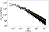 |
Fig. A.1. Power spectral density |


All Tables
Total energy losses and phenomenological estimates in the non-Alfvénic (NALF) and Alfvénic (ALF) streams.
All Figures
|
Fig. 1. Schematic view of the spectral evolution with distance of |
| In the text | |
|
Fig. 2. Overview of the selected intervals of fast and slow streams. Light green and green areas correspond to the fast Alfvénic and slow non-Alfvénic streams, respectively. From top to bottom: Solar wind speed, VSW (black), and magnetic field intensity, |B| (red); proton temperature, T (black), and proton density, n (red); correlation between magnetic and velocity fluctuations, CvB, at a 1 h scale. |
| In the text | |
|
Fig. 3. Second-order structure functions for the two Elsasser fields, 𝒮+ and 𝒮−, in black and red lines, respectively, for the non-Alfvénic interval. The component-anisotropic residual energy, 𝒮R in Eq. (18), is plotted in blue. A thin line is used for negative values and a thick line for positive ones. The dotted line is a reference for the Kolmogorov scaling, 𝒮 ∝ ℓ2/3. |
| In the text | |
|
Fig. 4. Cascade rate and expansion losses, 𝒦 and ℱexp, respectively, in green and blue lines, for the Elsasser field z+ and z− (top and bottom respectively) in the non-Alfvénic stream. Thick (thin) lines indicate positive (negative) values. |
| In the text | |
|
Fig. 5. Cascade and expansion losses for the total energy (left) and the cross helicity (right) for the non-Alfvénic stream. |
| In the text | |
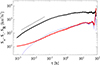 |
Fig. 6. Same as Fig. 3 but for the Alfvénic interval. |
| In the text | |
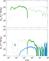 |
Fig. 7. Same as Fig. 4 but for the fast Alfvénic stream. |
| In the text | |
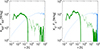 |
Fig. 8. Same as Fig. 5 but for the Alfvénic stream. |
| In the text | |
|
Fig. 9. Comparison between the measure cascade, 𝒦+, in the Alfvénic stream and two phenomenologies obtained using second-order structure functions: the Kolmogorov one plotted with a thin grey line and the Iroshnikov-Kraichnan one plotted with a thick grey line, Eqs. (29) and (30), respectively. |
| In the text | |
|
Fig. A.1. Power spectral density |
| In the text | |
Current usage metrics show cumulative count of Article Views (full-text article views including HTML views, PDF and ePub downloads, according to the available data) and Abstracts Views on Vision4Press platform.
Data correspond to usage on the plateform after 2015. The current usage metrics is available 48-96 hours after online publication and is updated daily on week days.
Initial download of the metrics may take a while.