| Issue |
A&A
Volume 685, May 2024
|
|
|---|---|---|
| Article Number | A85 | |
| Number of page(s) | 8 | |
| Section | The Sun and the Heliosphere | |
| DOI | https://doi.org/10.1051/0004-6361/202348810 | |
| Published online | 08 May 2024 | |
Improved reconstruction of solar magnetic fields from imaging spectropolarimetry through spatio-temporal regularisation⋆
Institute for Solar Physics, Dept. of Astronomy, Stockholm University, AlbaNova University Centre, 106 91 Stockholm, Sweden
e-mail: jaime@astro.su.se
Received:
1
December
2023
Accepted:
5
February
2024
Context. Determination of solar magnetic fields with a spatial resolution set by the diffraction limit of a telescope is difficult because the time required to measure the Stokes vector with sufficient signal-to-noise ratio is long compared to the solar evolution timescale. This difficulty becomes greater with increasing telescope size as the photon flux per diffraction-limited resolution element remains constant but the evolution timescale decreases linearly with the diffraction-limited resolution.
Aims. We aim to improve magnetic field reconstruction at the diffraction limit without averaging the observations in time or space, and without applying noise filtering.
Methods. The magnetic field vector tends to evolve more slowly than the temperature, velocity, or microturbulence. We exploit this by adding temporal regularisation terms for the magnetic field to the linear least-squares fitting used in the weak-field approximation, as well as to the Levenberg-Marquardt algorithm used in inversions. The other model parameters are allowed to change in time without constraints. We infer the chromospheric magnetic field from Ca II 854.2 nm observations using the weak field approximation and the photospheric magnetic field from Fe I 617.3 nm observations, both with and without temporal regularisation.
Results. Temporal regularisation reduces the noise in the reconstructed maps of the magnetic field and provides a better coherency in time in both the weak-field approximation and Milne-Eddington inversions.
Conclusions. Temporal regularisation markedly improves magnetic field determination from spatially and temporally resolved observations.
Key words: polarization / radiative transfer / Sun: chromosphere / Sun: magnetic fields / stars: atmospheres
Movies are available at https://www.aanda.org.
© The Authors 2024
 Open Access article, published by EDP Sciences, under the terms of the Creative Commons Attribution License (https://creativecommons.org/licenses/by/4.0), which permits unrestricted use, distribution, and reproduction in any medium, provided the original work is properly cited.
This article is published in open access under the Subscribe to Open model. Subscribe to A&A to support open access publication.
1. Introduction
The degree of polarisation in spectral lines induced by magnetic fields in the solar atmosphere can be higher than 10% in regions with strong field (e.g. Martinez Pillet et al. 1990; Castellanos Durán et al. 2020), but more commonly it is much lower: linear polarisation induced by the Zeeman and Hanle effect in lines formed in the chromosphere tends to be smaller than 0.1%, especially in the quiet Sun where field strengths are low (e.g. Jurčák et al. 2018; Centeno et al. 2021). Observations of the full Stokes vector therefore require long integration times and/or spatial averaging over areas larger than the diffraction limit of the telescope in order to reach the signal-to-noise ratio (S/N) required to detect signals with a strength of < 0.1% of the local continuum intensity (e.g. Centeno et al. 2010).
A major goal of modern solar telescopes is to perform such imaging spectropolarimetry at the diffraction limit. This goal is largely reliant on the calibration accuracy of the instruments. For example, the CRISP instrument at the Swedish 1-m Solar Telescope (Scharmer et al. 2003) can currently reach a polarimetric accuracy of ∼10−3 and the DKIST telescope can be calibrated to an accuracy of 5 × 10⁻⁴ (Rimmele et al. 2020).
Because of the finite brightness of the Sun, the S/N that is required to match the polarimetric accuracy is not reached instantaneously. For example, it takes 2 s to reach a S/N of 5 × 10⁻⁴ at the diffraction limit in the continuum adjacent to the Ca II 854.2 nm line at a spectral resolution of λ/Δλ = 80 000 and a total transmission of the telescope-instrument-camera chain of 5%. Tuneable-filter-based instruments, such as CRISP or VTF at DKIST, require data acquisition typically at 10 to 20 wavelengths, depending on the width of the line and the desired wavelength coverage. This leads to a total acquisition time of roughly 20 to 40 s for a diffraction-limited full-Stokes line scan.
This time is large compared to the timescale on which the density, temperature, and velocity in the atmosphere change: the sound-crossing time for a diffraction-limited pixel of a 1 m telescope at 854 nm is 9 s assuming a sound speed of 7 km s−1; for a 4 m telescope, this value is 2 s. The sound speed should be considered as a lower limit; in the chromosphere, the Alfvén speed is a better indicator of the evolution speed. This latter can be larger than 100 km s−1, implying changes of the thermodynamic parameters in less than 0.1 s.
Therefore, using diffraction-limited instruments based on tunable filters to reach the required high S/N inevitably leads to observed Stokes profiles that average different atmospheric states in density, temperature, and velocity. Using integral field spectropolarimeters, such as microlensed hyperspectral imagers (van Noort et al. 2022) or image slicers (Dominguez-Tagle et al. 2022), mitigates – but does not fully eliminate – this effect, but at the cost of a strongly reduced field of view (FOV).
This mismatch of required integration times and evolution timescales poses a severe problem for inferring chromospheric magnetic fields, especially over the large FOVs of Fabry-Pérot-type instruments. The equations that describe radiative transfer are non-linear. An inversion of a time-averaged line profile does not, in general, yield an inferred atmosphere that represents the time-average of the underlying atmosphere (Carlsson & Stein 1995). Time-averaging of the Stokes vector might even result in an observed average Stokes vector that cannot be reproduced by any single atmosphere model.
The magnetic field in the chromosphere, where the magnetic pressure is higher than the gas pressure, tends to be relatively smooth and to vary slowly over space. Morosin et al. (2020) realised that this property can be exploited to improve the inference of magnetic fields from noisy data using the weak-field approximation (WFA). These authors extended the merit function used in the WFA-fit with a term that penalises differences in magnetic field in neighbouring pixels, and showed that this leads to substantially improved inference of the longitudinal magnetic field based on the Mg I 517.3 nm, Na I 589.6 nm, and Ca II 854.2 nm lines.
The magnetic field in the chromosphere generally only evolves over granular turnover timescales of several minutes (Kleint 2017; Ferrente et al. 2023), but the mass density, temperature, and velocity evolve with a timescale of seconds on spatial scales of a few tens of kilometers. We propose to exploit this temporal smoothness to improve magnetic field inference from observations taken at or close to the diffraction limit.
The general idea is to perform inversions where, for the same spatial pixel, observations at consecutive time steps are allowed to have arbitrary variations in the velocity, temperature, and other variables that are well-constrained by Stokes I at relatively low S/N. The magnetic field, which is constrained by Stokes Q, U, and V and requires a high S/N to be constrained, should vary as little as possible while staying consistent with the data, given the noise level.
This concept can be viewed as applying Tikhonov regularisation (Tikhonov & Arsenin 1977; Willoughby 1979) to the magnetic field in the time domain. In the case of the WFA, this can be implemented as a straightforward extension of the method presented by Morosin et al. (2020). In the case of inference methods based on explicit radiative transfer, whether in the Milne-Eddington approximation (ME), LTE, or full non-LTE, inference methods can be implemented as an extension of the method described in de la Cruz Rodríguez (2019). The WFA is linear, and requires only a single matrix inversion to yield a solution; while the rest of the aforementioned inference methods are non-linear and can be solved using the Levenberg-Marquardt algorithm (LM, Levenberg 1944; Marquardt 1963).
In the present paper, we provide implementations for both cases. As a proof of concept, we apply the temporally regularised WFA to observations of quiet Sun in the Ca II 854.2 nm line, and apply temporally regularised ME inversions to observations of quiet Sun in the Fe I 617.3 nm line. We chose to illustrate the non-linear case with the ME approximation applied to a photospheric line because it is easy to implement and can be quickly inverted; the formalism also remains identical for LTE and non-LTE inversions of chromospheric lines.
The observations that we use here are obtained with a Fabry-Perot tunable-filter instrument. The individual line positions contained in the data are not taken simultaneously, but sequentially. We assume that one line scan comprises a time step that will be represented by one atmosphere model. As we mention above, this is an approximation, as the solar evolution timescale is smaller than the scan time, and this can translate into errors in the inferred model parameters (e.g. Felipe et al. 2018). We stress that temporal regularisation can also be used for integral-field spectropolarimeters. These record all wavelengths simultaneously, and the integration time used in a time step is mainly set by the desired S/N, and this time is significantly shorter than would be needed by a tunable-filter instrument.
2. Observations
We use two datasets acquired with the CRISP instrument (see Scharmer 2006; Scharmer et al. 2019; de Wijn et al. 2021) at the Swedish 1-m Solar Telescope. The datasets were reduced with the SSTRED pipeline (de la Cruz Rodríguez et al. 2015; Löfdahl et al. 2021), and processed with the MOMFBD algorithm to minimise atmospheric distortions (Löfdahl 2002; Van Noort et al. 2005). The polarimetric calibration was individually performed for each pixel as described in van Noort & Rouppe van der Voort (2008).
The first dataset, recorded on 14 July 2020 starting at 08:40 UT at disc centre, consists of a four-line program with data acquired in the Ca II 854.2 nm, Fe I 617.3 nm, Hα and Mg I 517.3 nm lines. We only used the 854.2 nm data in this study. The line was sampled between ±30 pm from line centre in regular steps of 7.5 pm, with a total integration time per wavelength of 0.91 s. The overall cadence – including all four lines – is 34.2 s, whereas the total acquisition time for one 854.2 nm scan was approximately 13 s. The upper row in Fig. 1 illustrates the four Stokes parameters in the first time step at +15 pm from line centre. The target is a quiet-Sun region that harbours two small network patches with opposite polarity. We estimated the noise level based on the outermost wavelength points. The standard deviations of the noise were found to be σQ, U, V = (3.9, 2.6, 2.7)×10−3.
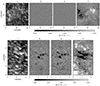 |
Fig. 1. Observations used in this study. Top: Stokes parameters in the Ca II 854.2 nm line at +15 pm from line centre. Bottom: Stokes parameters in the Fe I 617.3 nm line at −17.5 (I) and −7.0 pm (Q, U, V) from line centre. Stokes Q, U, and V have been normalised by the spatially averaged Stokes I intensity at the same wavelength. |
The second dataset, recorded on 26 May 2021 starting at 09:48 UT on coordinates (X, Y) = (698, 387) (μ = 0.54), consists of a patch of quiet Sun close to active region AR 12824. We recorded data in the Ca II 854.2 nm and Fe I 617.3 nm lines, but we only used the 617.3 nm data in this study. The Fe I 617.3 nm line was sampled at Δλ = [ − 17.5, − 10.5, − 7, − 3.5, 0, 3.5, 7, 10.5, 14, 17.5] pm from line centre, with a total integration time per wavelength of 0.28 s. The selected FOV is illustrated in the bottom row of Fig. 1 in all four Stokes parameters at −7 pm from line centre. The background noise as estimated from the continuum point has standard deviations of σQ, U, V = (1.8, 2.3, 2.5)×10−3.
3. Method
3.1. The linear case: Application to the weak-field approximation
When the dependence of the observable on the model parameters is linear, spatial and temporal regularisation can be trivially imposed. The weak-field approximation (Landi Degl’Innocenti & Landi Degl’Innocenti 1973; Jefferies et al. 1989) allows us to write analytical expressions for the Q, U, and V profiles that are linear in  and B∥.
We extend the implementation of Morosin et al. (2020) by also adding regularisation in the temporal dimension. In order to derive general expressions for the linear case, let us assume that we can express our synthetic prediction si of the ith data point in a pixel as si = ciP, where ci is a quantity that does not depend on the model parameters (but that can change for each data point) and P is a model parameter. For a given pixel at coordinates t, y, x, we can write the regularised merit function χ2 as:
![$$ \begin{aligned} \chi ^2 =&\frac{1}{N_{\mathrm{data} }}\sum _{i=1}^{N_{\mathrm{data} }}\left(\frac{o_{t,y,x}^i - c_iP_{t,y,x}}{\sigma _i}\right)^2 + \alpha \left[(P_{t,y,x} - P_{t,y,x-1})^2\right.\nonumber \\&\left.+ (P_{t,y,x} - P_{t,y,x+1})^2 + (P_{t,y,x} - P_{t,y-1,x})^2 + (P_{t,y,x} - P_{t,y+1,x})^2\right]\nonumber \\&+ \beta \left(P_{t,y,x} - P_0\right)^2 + \gamma \left[(P_{t,y,x} - P_{t-1,y,x})^2 + (P_{t,y,x} - P_{t+1,y,x})^2\right], \end{aligned} $$](/articles/aa/full_html/2024/05/aa48810-23/aa48810-23-eq2.gif)
where oi is the ith observed data point, α is a spatial regularisation weight, β is a low-norm regularisation weight that penalises deviations from a constant value P0 and γ is a temporal regularisation weight. Taking the derivative of Eq. (1) with respect to all Pt, y, x, and equating it to zero to find the minimum, while absorbing the scaling factors Ndata and σi into oi and ci, we can derive a sparse linear system of equations (AP = B), where the different temporal and spatial locations are coupled by the non-diagonal regularisation terms:
![$$ \begin{aligned} \left[\sum _i c_i^2 + 4\alpha + \beta \right]P_{t,y,x}&- \alpha \left(P_{t,y-1,x} + P_{t,y+1,x} + P_{t,y,x-1} + P_{t,y,x+1}\right)\nonumber \\&- \gamma \left(P_{t-1,y,x} + P_{t+1,y,x}\right) = \sum _i c_io_{t,y,x}^i + \beta P_0. \end{aligned} $$](/articles/aa/full_html/2024/05/aa48810-23/aa48810-23-eq3.gif)
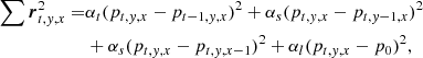
Equation (2) couples the parameters of the different pixels (Pt, y, x) through the regularisation weights (α, β, γ) on the left-hand side. Obtaining a solution requires that we solve a global problem for all pixels simultaneously. If the regularisation weights are zero, the A matrix in Eq. (2) is diagonal and we recover the unconstrained algorithm. Figure 2 shows the structure of A for a small FOV of 4 × 4 pixels and three time steps. Compared to Fig. 1 of Morosin et al. (2020), this matrix has two extra off-diagonal bands originating from the temporal regularisation terms.
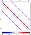 |
Fig. 2. Regularisation matrix for the linear case. Each row corresponds to the regularisation function for one pixel in space and time. For displaying purposes, we assume an observation with dimensions nt = 3, ny = 4, nx = 4 and regularisation weights α = 1, β = 1, and γ = 2.5. The outermost bands (darker blue) correspond to the temporal regularisation terms, whereas the inner light-blue terms originate from the spatial regularisation. |
If we replace Pt, y, x with  and ∑ici with ∑iC∂Ii/∂λi, we directly obtain the expression for the fully regularised WFA, with
 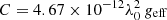 , λ0 the central wavelength of the line in nm, and geff the effective Landé factor of the transition.
Figure 3 illustrates a comparison of four reconstructions of B∥ from the Ca II 854.2 nm dataset using the unconstrained WFA algorithm, the spatially regularised method of Morosin et al. (2020), and two variants of our method that include temporal regularisation alone as well as both temporal and spatial regularisation. The reconstruction of the unconstrained algorithm has a very noisy background, and besides the magnetic field in the strong network patches, small-scale loop-like features can be discerned in the FOV. The inclusion of spatial regularisation greatly decreases the noise in the background, making the small-scale loop-like features much more visible compared to the unconstrained case. Temporal regularisation alone also decreases the noise, perhaps yielding a slightly sharper model than the spatially regularised one, while also decreasing the temporal fluctuations of the background noise along the time series. The combined action of temporal and spatial regularisation further decreases the noise compared to the previous cases and yields a model with the highest S/N. The standard deviation of the noise in the magnetic field, as measured in the lower-right corner of the image, is reduced from 18 G in the unconstrained case to 9 G in the fully regularised case. The improvement induced by spatial regularisation is particularly obvious in the movie showing the entire time series. The upper panel in Fig. 4 further illustrates the reduction of the noise in the regularised reconstructions along a slice through the FOV.
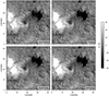 |
Fig. 3. Reconstructions of the line-of-sight component of the magnetic field (B∥), inferred by applying the weak-field approximation to the Ca II 854.2 nm data. Upper-left panel: reconstruction performed with the unconstrained algorithm. Lower-left panel: reconstruction performed with a temporally regularised algorithm. Lower-right panel: reconstruction performed with a spatially regularised algorithm. Upper-right panel: reconstruction performed with full regularisation in space and time. A movie with the time series is available https://www.aanda.org/10.1051/0004-6361/202348810/olm. The red tick marks indicate the location of the cut shown in Fig. 4. |
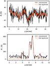 |
Fig. 4. Vertical cuts of the reconstructed magnetic field. The upper panel shows a reconstruction of B∥ with the weak-field approximation from the 854.2 nm dataset along a cut indicated with red markers in Fig. 3. The black curve shows the unconstrained reconstruction, and the red curve shows the reconstruction with both spatial and temporal regularisation. A similar plot is shown in the lower panel for the reconstruction of B⊥ from the ME inversion of the 617.3 nm dataset presented in Fig. 7. |
3.2. The non-linear case: Application to Milne-Eddington inversions
The LM algorithm is one of the most efficient methods for reconstructing the parameters of non-linear models from observations. Regularised LM implementations are used in different fields of astrophysics in order to constrain the parameters of the model under consideration (e.g. Piskunov & Kochukhov 2002; de la Cruz Rodríguez et al. 2019). The regularisation is represented by a set of Npen penalty functions rn(p) that are squared in order to have ℓ − 2 norm regularisation. Following the notation of de la Cruz Rodríguez et al. (2019), the merit function χ2 can generally be expressed as a function of the model parameter vector p and the data points x:
![$$ \begin{aligned} \chi ^2(\boldsymbol{p},\boldsymbol{x}) = \frac{1}{N_{\mathrm{data} }}\sum _{k=1}^{N_{\mathrm{data} }} \left[\frac{o_k-s(\boldsymbol{p},x_k)}{\sigma _k}\right]^2 + \sum _{n=1}^{N_{\mathrm{pen} }}\alpha _nr_n(\boldsymbol{p})^2, \end{aligned} $$](/articles/aa/full_html/2024/05/aa48810-23/aa48810-23-eq6.gif)
where the weights αn regulate the influence of the regularisation terms in the merit function. We note that, unlike in the linear case, the penalty functions are not independently defined for each pixel (see below).
The model corrections predicted by the regularised LM algorithm can be derived by linearising Eq. (3) and taking the derivative with respect to the model parameters. The correction to the model parameters (Δp), in vector form, is given by a linear system of equations:

where J is the Jacobian matrix of the model and L is the Jacobian matrix of the penalty functions. In this expression, all constants and normalising factors are implicitly contained in the corresponding vectors. For any given parameter pt, y, x, the regularisation functions are defined as:
where we have included spatial, temporal, and low-norm regularisation terms.
If the penalty functions have a linear dependence on the model parameters, as in the ones used in this study, we can express them as r = Lp + c, where the coupling is contained in the Jacobian matrix L. Figure 5 illustrates the structure of L for a problem with nt = 3, ny = 4, nx = 4, and npar = 2. The maximum number of penalty functions should be npen < 4nxnynt, as some functions are not defined at the edges of the problem. Figure 6 illustrates the approximate Hessian matrix of the regularisation functions L ⋅ LT. The size of the approximate Hessian matrix is set by the total number of free parameters of the problem, which is also the size of one row of the LT matrix (4 × 4 × 3 × 2 = 96). In the latter, the outer dark blue bands originate from the temporal regularisation, whereas the inner light-blue bands contain the spatial coupling terms. For npar = 1, this matrix is identical in form to that shown in Fig. 2 for the linear case.
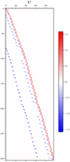 |
Fig. 5. Transpose of the Jacobian matrix of the penalty functions for the non-linear case with nt = 3, ny = 4, nx = 4, npar = 2, and regularisation weights α = 1, β = 1, and γ = 2.5. Each row corresponds to one penalty function and each column indicates the free parameters that are affected. |
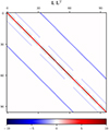 |
Fig. 6. Hessian approximation of the regularisation functions (LTL). This matrix was computed using L from Fig. 5. |
In this case, we are only including penalty functions that compare a parameter value with its neighbouring values at t − 1, y − 1, and x − 1. However, because the product L ⋅ LT is similar to a correlation of each penalty function with all others, the resulting coupling matrix in the left-hand side has identical structure to that in the linear case where we also include explicit comparisons with the values at t + 1, y + 1, and x + 1.
In a previous study, de la Cruz Rodríguez (2019) implemented a multi-resolution inversion code that included spatial regularisation and allowed us to deal with the effects of the telescope point spread function in ME inversions (PyMilne1). We extended this code to include temporal regularisation terms. With these changes, the code can now invert a time series of maps as a global problem. We inverted a time-series of 14 line scans acquired in the Fe I 617.3 nm line in a quiet-Sun patch. These observations are not ideal because they also include scans in the Ca II 854.2 nm line, inducing a time gap between consecutive Fe I scans. Nevertheless, the cadence is sufficiently high to illustrate the advantages of the method. In the following, we focus on the reconstruction of B⊥, which is a more challenging problem than reconstructing B∥.
We performed reconstructions with the unconstrained algorithm, including spatial regularisation only, temporal regularisation only, and a case including low-norm, spatial, and temporal regularisation altogether. Regularisation was only imposed in the three components of the magnetic field, leaving all other parameters unconstrained. Therefore, the thermodynamical quantities of the model are allowed to change freely in time and space.
Figure 7 compares reconstructions of the time series of B⊥ from the unconstrained algorithm and the three regularised cases. The improvements of the fully regularised reconstruction are threefold:
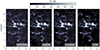 |
Fig. 7. Reconstruction of the transverse component of the magnetic field vector from ME inversions of the Fe I 617.3 nm. Left: unconstrained reconstruction where each pixel has been inverted six times with five different random initialisations. Middle-left: reconstruction with spatial regularisation, where all pixels have only been inverted once. Middle-right: reconstruction with temporal regularisation. Right: reconstruction including temporal, spatial, and low-norm regularisation terms. A movie with the time-evolution is available https://www.aanda.org/10.1051/0004-6361/202348810/olm. |
-
So-called inversion noise – caused by pixels where the algorithm did not converge to the global minimum – is absent. This effect is clearest in the patches of strong magnetic field, where randomly located black pixels are present in the unconstrained reconstruction. Examples of inversion noise are also visible in the lower panel of Fig. 4 at y ≈ 3.7″ and y ≈ 4.35″. Inversion noise can be removed from the unconstrained method by initialising the inversion several times with different starting model parameters or by performing a two-cycle inversion with a smoothing step in between (as suggested by Milić & van Noort 2018). However, the noise is naturally addressed in all the regularised cases, where the coupling between pixels in space and/or time removes it entirely.
-
There is a reduction of the background noise bias level. The presence of noise in the observations can manifest as a non-zero background bias-level for parameters that are defined positive (see Martínez González et al. 2012). We find that all forms of regularisation decrease this bias, but the low-norm regularisation term (with P0 = 0) and the temporal regularisation are particularly effective in this regard. The spatially regularised time series shows a stronger frame-to-frame fluctuation in the background level, which seems to be induced by varying atmospheric seeing conditions along the series. This effect is also visible in the lower panel of Fig. 4, where the red curve is regularly predicting much lower values of B⊥ in regions located between stronger network patches.
-
The time coherence of weak magnetic structures is enhanced. Structures with signal barely above the noise appear more persistent in time with temporal regularisation. Without this regularisation, they appear intermittently, only in those time steps where the noise happens to be low enough for the inversion to pick up the structure.
However, despite these improvements, the evolution of magnetic fields in the photosphere is anchored to the forces originating from gas-pressure gradients (plasma β ≫ 1), and our assumption that the magnetic field is slowly evolving relative to the other parameters is not optimal. Compared to the chromospheric case presented in Sect. 3.1, we had to limit the amount of temporal regularisation to perform these inversions.
4. Discussion and conclusions
We present a method to include Tikhonov regularisation in the time dimension for linear and non-linear fits of model parameters. We show that this method is suitable for improving determinations of the magnetic field in the solar chromosphere.
Compared to other techniques that operate on the data to decrease noise, such as temporal and spatial rebinning, principal component analysis filtering (see e.g. Martínez González et al. 2008), Fourier filtering, or neural-network-based noise reduction (Díaz Baso et al. 2019), regularisation leaves the data untouched and operates only on the model parameters. This is an important advantage because filtering and/or averaging the data likely affects the reconstruction of all parameters, whether that is desired or not.
Temporal regularisation addresses the different timescales on which the magnetic field and the thermodynamical parameters evolve in the chromosphere as well as the different S/N required to constrain them. Because the thermodynamic parameters evolve relatively quickly but require a low S/N, one can use zero (as we do here) or weak regularisation. The magnetic field evolves more slowly but requires high S/N, and is therefore regularised more strongly.
Choosing adequate regularisation weights is crucial to obtain results that are not overly smooth. The weights must be chosen in such a way that the final quality of the fit is not affected; a threshold value should be chosen above which the quality of the fits starts to be negatively affected by the limitations imposed by the regularisation terms (Kochukhov 2017). For observations with low S/N, this might mean that the regularisation is so strong that it makes the magnetic field almost constant in time. We emphasise that with properly chosen weights, regularisation does not guarantee that the magnetic field will be constant over time; if the S/N is sufficiently high, it still allows sharp gradients in time. However, in cases of intermediate S/N, regularisation will produce smoother solutions if strong gradients are not required to minimise χ2. Regularisation has an advantage over smoothing the model parameters after an unconstrained inversion, because smoothing washes out variations regardless of the impact that they have on χ2, but regularisation maintains sharp gradients in locations where they have a significant impact in χ2.
Most observational programs with Fabry-Perot instruments that observe multiple lines are carried out by scanning once through each line and repeating this cycle. Long integration times are needed for chromospheric lines in order to reach sufficient S/N to measure polarisation. As mentioned in the introduction, this takes about 20 s, and the observed line profile is not produced by a single atmosphere as the Sun has evolved over this time.
Temporal regularisation allows observing strategies that mitigate this problem. Instead of a single slow scan, one can perform multiple fast scans that each have sufficient S/N to constrain the thermodynamic parameters. These profiles now suffer less from solar evolution and therefore lead to improved reconstructions of the thermodynamic parameters. Temporal regularisation of the magnetic field couples the scans together and increases the “effective” S/N sufficiently to determine the field. These fast scans can be interleaved with observations in other lines (which themselves can consist of multiple scans) as needed, as temporal regularisation does not require a constant cadence. If needed, the temporal regularisation weight can be made smaller for scans that are not performed back-to-back.
Another obvious application is to data taken with integral-field spectropolarimeters. Here the assumptions behind temporal regularisation hold much better, because all spatial and spectral datapoints are taken simultaneously, and the cadence is typically high (Rouppe van der Voort et al. 2023).
Data taken at the diffraction limit of a telescope have a limited S/N if the exposure time is kept short enough to prevent solar evolution from blurring the images. Spatio-temporal regularisation of the magnetic field is a way of increasing the effective S/N of the data while keeping exposure times short. This technique will be invaluable when considering data taken with large-aperture telescopes, such as DKIST (Rimmele et al. 2020) and the planned EST (Quintero Noda et al. 2022).
The version of pyMilne that includes temporal regularisation is available in the official repository1. The regularised WFA code used here is also publicly available2.
Movies
Movie 1 associated with Fig. 3 (WFA) Access here
Movie 2 associated with Fig. 7 (ME_inversion) Access here
Acknowledgments
The authors of this paper are thankful to the referee for his careful evaluation of the manuscript. The Institute for Solar Physics is supported by a grant for research infrastructures of national importance from the Swedish Research Council (registration number 2021-00169). The Swedish 1-m Solar Telescope is operated on the island of La Palma by the Institute for Solar Physics of Stockholm University in the Spanish Observatorio del Roque de los Muchachos of the Instituto de Astrofísica de Canarias. J.L. acknowledges financial support from the Swedish Research council (VR, project number 2022-03535). This project has been funded by the European Union through the European Research Council (ERC) under the Horizon Europe program (MAGHEAT, grant agreement 101088184).
References
- Carlsson, M., & Stein, R. F. 1995, ApJ, 440, L29 [Google Scholar]
- Castellanos Durán, J. S., Lagg, A., Solanki, S. K., & van Noort, M. 2020, ApJ, 895, 129 [Google Scholar]
- Centeno, R., Trujillo Bueno, J., & Asensio Ramos, A. 2010, ApJ, 708, 1579 [NASA ADS] [CrossRef] [Google Scholar]
- Centeno, R., de la Cruz Rodríguez, J., & del Pino Alemán, T. 2021, ApJ, 918, 15 [NASA ADS] [CrossRef] [Google Scholar]
- de la Cruz Rodríguez, J. 2019, A&A, 631, A153 [NASA ADS] [CrossRef] [EDP Sciences] [Google Scholar]
- de la Cruz Rodríguez, J., Löfdahl, M. G., Sütterlin, P., Hillberg, T., & Rouppe van der Voort, L. 2015, A&A, 573, A40 [NASA ADS] [CrossRef] [EDP Sciences] [Google Scholar]
- de la Cruz Rodríguez, J., Leenaarts, J., Danilovic, S., & Uitenbroek, H. 2019, A&A, 623, A74 [Google Scholar]
- de Wijn, A. G., de la Cruz Rodríguez, J., Scharmer, G. B., Sliepen, G., & Sütterlin, P. 2021, AJ, 161, 89 [NASA ADS] [CrossRef] [Google Scholar]
- Díaz Baso, C. J., de la Cruz Rodríguez, J., & Danilovic, S. 2019, A&A, 629, A99 [NASA ADS] [CrossRef] [EDP Sciences] [Google Scholar]
- Dominguez-Tagle, C., Collados, M., Lopez, R., et al. 2022, J. Astron. Instrum., 11, 2250014 [NASA ADS] [CrossRef] [Google Scholar]
- Felipe, T., Socas-Navarro, H., & Przybylski, D. 2018, A&A, 614, A73 [NASA ADS] [CrossRef] [EDP Sciences] [Google Scholar]
- Ferrente, F., Zuccarello, F., Guglielmino, S. L., Criscuoli, S., & Romano, P. 2023, ApJ, 954, 185 [NASA ADS] [CrossRef] [Google Scholar]
- Jefferies, J., Lites, B. W., & Skumanich, A. 1989, ApJ, 343, 920 [Google Scholar]
- Jurčák, J., Štěpán, J., Trujillo Bueno, J., & Bianda, M. 2018, A&A, 619, A60 [NASA ADS] [CrossRef] [EDP Sciences] [Google Scholar]
- Kleint, L. 2017, ApJ, 834, 26 [Google Scholar]
- Kochukhov, O. 2017, A&A, 597, A58 [NASA ADS] [CrossRef] [EDP Sciences] [Google Scholar]
- Landi Degl’Innocenti, E., & Landi Degl’Innocenti, M. 1973, Sol. Phys., 31, 299 [CrossRef] [Google Scholar]
- Levenberg, K. 1944, Q. Appl. Math., 2, 164 [Google Scholar]
- Löfdahl, M. G. 2002, in Image Reconstruction from Incomplete Data, eds. P. J. Bones, M. A. Fiddy, & R. P. Millane, SPIE Conf. Ser., 4792, 146 [CrossRef] [Google Scholar]
- Löfdahl, M. G., Hillberg, T., de la Cruz Rodríguez, J., et al. 2021, A&A, 653, A68 [Google Scholar]
- Marquardt, D. 1963, J. Soc. Ind. Appl. Math., 11, 431 [Google Scholar]
- Martínez González, M. J., Asensio Ramos, A., Carroll, T. A., et al. 2008, A&A, 486, 637 [NASA ADS] [CrossRef] [EDP Sciences] [Google Scholar]
- Martínez González, M. J., Manso Sainz, R., Asensio Ramos, A., & Belluzzi, L. 2012, MNRAS, 419, 153 [CrossRef] [Google Scholar]
- Martinez Pillet, V., Garcia Lopez, R. J., del Toro Iniesta, J. C., et al. 1990, ApJ, 361, L81 [NASA ADS] [CrossRef] [Google Scholar]
- Milić, I., & van Noort, M. 2018, A&A, 617, A24 [Google Scholar]
- Morosin, R., de la Cruz Rodríguez, J., Vissers, G. J. M., & Yadav, R. 2020, A&A, 642, A210 [NASA ADS] [CrossRef] [EDP Sciences] [Google Scholar]
- Piskunov, N., & Kochukhov, O. 2002, A&A, 381, 736 [NASA ADS] [CrossRef] [EDP Sciences] [Google Scholar]
- Quintero Noda, C., Schlichenmaier, R., Bellot Rubio, L. R., et al. 2022, A&A, 666, A21 [NASA ADS] [CrossRef] [EDP Sciences] [Google Scholar]
- Rimmele, T. R., Warner, M., Keil, S. L., et al. 2020, Sol. Phys., 295, 172 [Google Scholar]
- Rouppe van der Voort, L. H. M., van Noort, M., & de la Cruz Rodríguez, J. 2023, A&A, 673, A11 [NASA ADS] [CrossRef] [EDP Sciences] [Google Scholar]
- Scharmer, G. B. 2006, A&A, 447, 1111 [NASA ADS] [CrossRef] [EDP Sciences] [Google Scholar]
- Scharmer, G. B., Bjelksjo, K., Korhonen, T. K., Lindberg, B., & Petterson, B. 2003, in Innovative Telescopes and Instrumentation for Solar Astrophysics, eds. S. L. Keil, & S. V. Avakyan, SPIE Conf. Ser., 4853, 341 [NASA ADS] [CrossRef] [Google Scholar]
- Scharmer, G. B., Löfdahl, M. G., Sliepen, G., & de la Cruz Rodríguez, J. 2019, A&A, 626, A55 [NASA ADS] [CrossRef] [EDP Sciences] [Google Scholar]
- Tikhonov, A. N., & Arsenin, V. Y. 1977, Solutions of Ill-Posed Problems (New York: V. H. Winston& Sons) [Google Scholar]
- Van Noort, M., Rouppe Van Der Voort, L., & Löfdahl, M. G. 2005, Sol. Phys., 228, 191 [NASA ADS] [CrossRef] [Google Scholar]
- van Noort, M. J., & Rouppe van der Voort, L. H. M. 2008, A&A, 489, 429 [NASA ADS] [CrossRef] [EDP Sciences] [Google Scholar]
- van Noort, M., Bischoff, J., Kramer, A., Solanki, S. K., & Kiselman, D. 2022, A&A, 668, A149 [NASA ADS] [CrossRef] [EDP Sciences] [Google Scholar]
- Willoughby, R. A. 1979, SIAM Rev., 21, 266 [CrossRef] [Google Scholar]
All Figures
|
Fig. 1. Observations used in this study. Top: Stokes parameters in the Ca II 854.2 nm line at +15 pm from line centre. Bottom: Stokes parameters in the Fe I 617.3 nm line at −17.5 (I) and −7.0 pm (Q, U, V) from line centre. Stokes Q, U, and V have been normalised by the spatially averaged Stokes I intensity at the same wavelength. |
| In the text | |
|
Fig. 2. Regularisation matrix for the linear case. Each row corresponds to the regularisation function for one pixel in space and time. For displaying purposes, we assume an observation with dimensions nt = 3, ny = 4, nx = 4 and regularisation weights α = 1, β = 1, and γ = 2.5. The outermost bands (darker blue) correspond to the temporal regularisation terms, whereas the inner light-blue terms originate from the spatial regularisation. |
| In the text | |
|
Fig. 3. Reconstructions of the line-of-sight component of the magnetic field (B∥), inferred by applying the weak-field approximation to the Ca II 854.2 nm data. Upper-left panel: reconstruction performed with the unconstrained algorithm. Lower-left panel: reconstruction performed with a temporally regularised algorithm. Lower-right panel: reconstruction performed with a spatially regularised algorithm. Upper-right panel: reconstruction performed with full regularisation in space and time. A movie with the time series is available https://www.aanda.org/10.1051/0004-6361/202348810/olm. The red tick marks indicate the location of the cut shown in Fig. 4. |
| In the text | |
|
Fig. 4. Vertical cuts of the reconstructed magnetic field. The upper panel shows a reconstruction of B∥ with the weak-field approximation from the 854.2 nm dataset along a cut indicated with red markers in Fig. 3. The black curve shows the unconstrained reconstruction, and the red curve shows the reconstruction with both spatial and temporal regularisation. A similar plot is shown in the lower panel for the reconstruction of B⊥ from the ME inversion of the 617.3 nm dataset presented in Fig. 7. |
| In the text | |
|
Fig. 5. Transpose of the Jacobian matrix of the penalty functions for the non-linear case with nt = 3, ny = 4, nx = 4, npar = 2, and regularisation weights α = 1, β = 1, and γ = 2.5. Each row corresponds to one penalty function and each column indicates the free parameters that are affected. |
| In the text | |
|
Fig. 6. Hessian approximation of the regularisation functions (LTL). This matrix was computed using L from Fig. 5. |
| In the text | |
|
Fig. 7. Reconstruction of the transverse component of the magnetic field vector from ME inversions of the Fe I 617.3 nm. Left: unconstrained reconstruction where each pixel has been inverted six times with five different random initialisations. Middle-left: reconstruction with spatial regularisation, where all pixels have only been inverted once. Middle-right: reconstruction with temporal regularisation. Right: reconstruction including temporal, spatial, and low-norm regularisation terms. A movie with the time-evolution is available https://www.aanda.org/10.1051/0004-6361/202348810/olm. |
| In the text | |
Current usage metrics show cumulative count of Article Views (full-text article views including HTML views, PDF and ePub downloads, according to the available data) and Abstracts Views on Vision4Press platform.
Data correspond to usage on the plateform after 2015. The current usage metrics is available 48-96 hours after online publication and is updated daily on week days.
Initial download of the metrics may take a while.