| Issue |
A&A
Volume 689, September 2024
|
|
|---|---|---|
| Article Number | A45 | |
| Number of page(s) | 20 | |
| Section | Interstellar and circumstellar matter | |
| DOI | https://doi.org/10.1051/0004-6361/202348660 | |
| Published online | 30 August 2024 | |
Warped disk evolution in grid-based simulations
Zentrum für Astronomie, Heidelberg University,
Albert-Ueberle-Str. 2,
69120
Heidelberg,
Germany
e-mail: mail@carolin.kim
Received:
17
November
2023
Accepted:
23
May
2024
Context. Multiple observations have offered evidence that a significant fraction of protoplanetary disks contain warps. A warp in a disk evolves over time, affecting the appearance and shape of shadows and arcs. It also greatly influences kinematic signatures. Understanding warp evolution helps provide valuable insights into its origins.
Aims. Thus far, numerous theoretical studies of warped disks have been conducted using methods based on smoothed particle hydrodynamics (SPH). In our approach, we use a grid-based method in spherical coordinates, which offers notable advantages. For instance, it allows for an accurate modeling of low viscosity values. Furthermore, the resolution does not depend on density or mass of the disk and permits surface structures to be resolved.
Methods. We performed 3D simulations using FARGO3D to simulate the evolution of a warped disk and compared the results to 1D models. We extensively investigated the applicability of grid-based methods to misaligned disks and tested their dependence on the grid resolution as well as the disk viscosity.
Results. We find that grid-based hydrodynamic simulations are capable of simulating disks not aligned to the grid geometry. Our 3D simulation of a warped disk offers an apt comparison with 1D models in terms of the evolution of inclination. However, we also found a twist that is not captured in 1D models. After thorough analysis, we suspect this to be a physical effect possibly caused by non-linear effects neglected in the 1D equations. Evaluating the internal dynamics, we found sloshing and breathing motions, as predicted in local shearing box analysis. They may become supersonic, possibly leading to strong consequences for kinematic observations.
Conclusions. Warped disks can be accurately modeled in 3D grid-based hydrodynamics simulations when using a reasonably good resolution, especially in the θ-direction. We find a good agreement with the linear approximation of the sloshing motion, which highlights the reliability of 1D models.
Key words: accretion, accretion disks / hydrodynamics / protoplanetary disks
© The Authors 2024
 Open Access article, published by EDP Sciences, under the terms of the Creative Commons Attribution License (https://creativecommons.org/licenses/by/4.0), which permits unrestricted use, distribution, and reproduction in any medium, provided the original work is properly cited.
This article is published in open access under the Subscribe to Open model. Subscribe to A&A to support open access publication.
1 Introduction
As more and more observations of protoplanetary disks become available (Andrews et al. 2018; Andrews 2020; Garufi et al. 2022, etc.), it is striking to note how many of them display non-axisymmetric features, such as the bright arcs as in HD 143006 (Pérez et al. 2018) or HD 135344B (Cazzoletti et al. 2018), spirals as in MWC 758 (Benisty et al. 2015), narrow shadow lanes as in HD 142527 (Marino et al. 2015) and in HD 135344B (Stolker et al. 2017), or the wide shaded regions as in TW Hydra (Debes et al. 2017) and in HD 139614 (Muro-Arena et al. 2020). Some of these asymmetrical features, in especially shadow lanes and wide shaded regions, can be traced back to a misaligned part of the disk casting a shadow.
Several misaligned disks have been detected, for instance: HD 142527 (Casassus et al. 2015), HD 100453 (Benisty et al. 2017), HD 143006 (Benisty et al. 2018), DoAr 44 (Casassus et al. 2018), GW Orionis (Kraus et al. 2020; Smallwood et al. 2021), KH 15D (Lodato & Facchini 2013; Poon et al. 2021), and many more. Bohn et al. (2022) specifically targeted disks with shadow features and measured the misalignment angle between inner and outer regions of the disk by looking at each disk in near-infrared (NIR) observations to probe the inner disk and submillimeter interferometric observations for the outer disk. Out of a sample of 20 disks, they found six disks with a significant misalignment and five disks showing no misalignment, while the remaining nine disks could not be analyzed with sufficient certainty based on the current data. A study by Min et al. (2017), involving analytical considerations of shadow locations, was used to deduce inner disk geometries. To investigate the shadow morphology, Nealon et al. (2019) studied shadows in synthetic scattered light observations. Nealon et al. (2020b) found that shadows cast by a misaligned inner disk can move in time and appear to rock back and forth depending on the misalignment angle and other disk geometry properties.
Misaligned disks can be classified into so-called “broken disks” that have two or more parts of the disk misaligned with respect to each other, and “warped disks,” which contain a continuous misalignment, meaning that all parts of the disk are connected and the inclination angle changes with radius. The classification is, however, not perfectly sharp as there can be objects falling in between those categories or a mixture of both.
There are multiple mechanisms leading to the formation of misaligned disks. In all cases, a misaligned component, either external, internal, or a mix of both, is exerting a torque on the disk. In one scenario, a binary misaligned with respect to the disk plane, gravitationally torques the disk. The misalignment can form in a circumprimary or secondary disk with an outer companion (Papaloizou et al. 1995; Zanazzi & Lai 2018a), as well as in a circumbinary disk (Facchini et al. 2013; Lodato & Facchini 2013; Zanazzi & Lai 2018b; Deng & Ogilvie 2022). In the case of an inclined outer companion, the disk can (under certain conditions) precesses as a rigid body (Papaloizou & Terquem 1995; Papaloizou et al. 1997) or break (Doğgan et al. 2023; Rabago et al. 2024). An inner companion can drive a warp, leading to the alignment of the disk with the binary orbital plane (Foucart & Lai 2013) or polar alignment (Zanazzi & Lai 2018b; Rabago et al. 2023). The disk can also get warped if the companion is not bound to the system but, instead, passing by in a so-called “fly-by” event (Clarke & Pringle 1993; Cuello et al. 2018; Nealon et al. 2020a). A misaligned planet can also cause a warp (Nealon 2018). This scenario is similar to the misaligned binary case, however with much smaller masses of the perturber. Such a misaligned planet could have been captured by the star-disk system or kicked out of the disk plane by N-body interaction with other objects, such as other planets or fly-by objects (Nagasawa et al. 2008). Late infall of material onto a disk could be another cause for a warp (Kuffmeier et al. 2021). In this scenario, the infalling material adds angular momentum with a different direction to the disk. Warped disks in combination with infalling material have also been observed (Sai et al. 2020). Additionally, the warping of disks has been found to affect planet formation (Aly et al. 2021).
In warped disks, pressure forces occur that act to change the disk’s orbital plane which means that a warped disk without a component driving the warp is not static but evolves in time (Papaloizou & Lin 1995; Papaloizou & Pringle 1983). The type of evolution depends on the disk properties, namely, the viscosity described by the Shakura-Sunyaev turbulence parameter, αt (Shakura & Sunyaev 1973) and its thickness, or (more specifically) its aspect ratio h = hp/r, where hp is the pressure scale height of the disk and r the distance from the star. Disks with high viscosity compared to the aspect ratio αt > h evolve in a diffusive manner. In this regime, the warp is directly dampened and dissipates (Pringle 1992; Ogilvie 1999; Lodato & Price 2010). Disks with lower viscosity, namely, αt < h, fall in the so-called wave-like regime. In this regime, the warp travels as a wave through the disk with a wave speed of cs/2 (Lubow & Ogilvie 2000; Gammie et al. 2000; Ogilvie & Latter 2013a,b). Over time, the warp is dampened as well in this regime, if αt ≠ 0. Because protoplanetary disks are known to have low viscosities of αt = 10−5−10−3 (Manara et al. 2023), they typically fall into the wave-like regime.
Historically, each evolution regime was described by a different set of equations for the warp evolution. Martin et al. (2019) were able to combine both equation sets to a generalized formalism. In their generalized set of equations, they included a damping term in order to suppress unphysical features. This damping term causes the equations to become stiff and challenging to solve numerically. Dullemond et al. (2022) (hereinafter referred to as DKZ22) were able to derive the same set of equations from shearing box considerations and found the reason for these unphysical features, as the equations need to take the rotation of the orbital plane into account. They proposed an alternative, physically motivated term to correct for the orbital plane rotation. The generalized equation set includes mass and angular momentum conservation, both of which depend on the internal torque vector, G. The equations are as follows:
![$\[\frac{\partial \Sigma}{\partial t}-\frac{2}{r} \frac{\partial}{\partial r}\left[\frac{\frac{\partial(r G)}{\partial r} \cdot \boldsymbol{l}}{r \Omega}\right]=0,\]$](/articles/aa/full_html/2024/09/aa48660-23/aa48660-23-eq1.png) (1)
(1)
![$\[\frac{\partial \boldsymbol{L}}{\partial t}-\frac{2}{r} \frac{\partial}{\partial r}\left[\frac{\frac{\partial(r \boldsymbol{G})}{\partial r} \cdot \boldsymbol{l}}{\sum r \Omega} \boldsymbol{L}\right]+\frac{1}{r} \frac{\partial(r \boldsymbol{G})}{\partial r}=T.\]$](/articles/aa/full_html/2024/09/aa48660-23/aa48660-23-eq2.png) (2)
(2)
Here, ∑ is the surface density, Ω the Kepler orbital frequency and L = ∑R2Ωl is the angular momentum density, with l as the angular momentum unit vector. The internal torque vector G arises due to the misalignment of neighbouring orbits (DKZ22) and takes the form:
![$\[\begin{aligned}\frac{\partial \boldsymbol{G}}{\partial t}+\left(\frac{\kappa^2-1}{2}\right) \Omega ~\boldsymbol{l} \times \boldsymbol{G} & +\alpha_{\mathrm{t}} \Omega \boldsymbol{G}+\left(\boldsymbol{l} \times \frac{\partial \boldsymbol{l}}{\partial t}\right) \times \boldsymbol{G} \\& =-\frac{\Omega^3 r \Sigma h_{\mathrm{p}}^2}{4} \frac{\partial \boldsymbol{l}}{\partial \ln r}+\frac{3}{2} \alpha_{\mathrm{t}}^2 \Omega^3 r \Sigma h_{\mathrm{p}}^2 \boldsymbol{l},\end{aligned}\]$](/articles/aa/full_html/2024/09/aa48660-23/aa48660-23-eq3.png) (3)
(3)
where κ = Ωe/Ω with Ωe as epicyclic frequency. We note that we are using the definition of the internal torque vector G and the notation following DKZ22, which differs from the definition given in other works, for instance, Martin et al. (2019) or Nixon & King (2016), by a factor of −1/r (see DKZ22, Appendix C).
As mentioned, the internal torque arises due to the misalignment of neighbouring orbits. More specifically, the annuli are deformed (see DKZ22, Fig. 9) and, therefore, they put pressure on neighbouring annuli. This leads to a dynamic surface where material flows radially inward and outward within one orbit. This motion is called sloshing motion (DKZ22), often referred to as “resonant motion” in the literature (Nixon & King 2016). The sloshing motion is the main drive for warp evolution.
Warped disks can be investigated in one-dimensional (1D) and three-dimensional (3D) models. In 1D models, the disk is to split into concentric annuli. Each annulus plane can be described by its normal vector, which is identical to the angular momentum unit vector. This angular momentum unit vector can then be updated following Eq. (2). While 1D models offer a huge advantage in regard to computation time, they are obviously simplified. Additionally, the equations are derived from a linear approximation and contain additional assumptions, for instance, about their Keplerity. Therefore, it is useful to model warped disks in full 3D hydrodynamic simulations.
Three-dimensional simulations of warped disks are often performed using smoothed particle hydrodynamics (SPH) models (Gingold & Monaghan 1977). However, the SPH method is usually implemented with an artificial viscosity that allows for shock treatment (Monaghan 2005). Simulations of disks modeled in SPH need to have a disk viscosity higher than the artificial viscosity in order to capture the physical processes accurately. Protoplanetary disks, however, are known to have a rather low viscosity (Pinte et al. 2016; Villenave et al. 2020), which means that a method able to model lower viscosities would be more fitting. Additionally, in the most common SPH models, the resolution highly depends on density. For a protoplanetary disk, this means that the surface of the disk is always less resolved than its midplane. For warped disks, however, it is advantageous to resolve the surface structures and dynamics well due to the sloshing motion mechanism. More importantly, observations of protoplanetary disks often trace the surface layers, which is why accurate model predictions for these regions are important.
In this work, we model warped disks in full 3D hydrodynamics using a grid-based code. This way, we are able to model protoplanetary disks with low viscosities, without the resolution dependency on density or any other physical quantity. However, we are aware that a grid can also cause numerical effects, as found by Hopkins (2015), for instance (see Fig. 8 therein). Thus, to minimize them, we chose a spherical symmetry of the grid to take advantage of the disk’s symmetry. As we still expect some numerical effects caused by the grid, we carefully tested the set-up in the test case of a planar and smooth disk inclined with respect to the grid geometry. Physically, this should give the same result as a planar disk aligned to the grid geometry and allow us to compare and extract the grid effects. A few studies used grid-based methods to model disks with out-of-plane features before (Sorathia et al. 2013; Fragner & Nelson 2010; Rabago et al. 2024, 2023).
This paper is organized as follows. We describe our numerical set-up in Sec. 2 and the investigation of the grid effects in the case of a disk tilted with respect to the midplane in Sec. 3. We present and discuss the results of a warped disk simulation in Sec. 4. In Sec. 5, we investigate the internal torque and sloshing motion in the 3D simulation. We present our conclusions in Sec. 6.
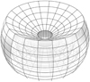 |
Fig. 1 Schematics of the spherical grid set-up in our simulations. The poles are cut off in order to save computation time. |
2 Numerical method
We performed 3D hydrodynamic simulations using the versatile code FARGO3D by Benítez-Llambay & Masset (2016). In our simulations, we used the implemented hydrodynamics modeling a system, consisting of a central star and a surrounding disk. For our purposes, we did not consider any magnetic fields and, therefore, we did not use the magnetohydrodynamic features of FARGO3D. Furthermore, we did not include any planets or other companions.
To take advantage of the system’s symmetry, we set up a model in spherical coordinates. To save on computation time, we restricted the vertical computation domain to a certain range, meaning that the poles of the grid sphere are cut off (see Fig. 1). Because we are planning to look at features tilted with respect to the midplane of the grid, we need to consider a large enough regime in the vertical direction.
We set up a protoplanetary disk, where the surface density follows the following power law:
![$\[\Sigma(r)=\Sigma_0\left(\frac{r}{R_0}\right)^{-p},\]$](/articles/aa/full_html/2024/09/aa48660-23/aa48660-23-eq4.png) (4)
(4)
with a slope, p, and reference scale, R0. In FARGO3D, this reference scale is usually set to R0 = 5.2 au, which we adopt in our models. In general, we assume a locally isothermal disk, which means that the temperature structure does not change in time. However, the temperature may very well vary within the disk and is not constant as a function of distance to the star. We set the temperature structure so that the disk is flared, such that the aspect ratio can be described as:
![$\[h(r)=h_0\left(\frac{r}{R_0}\right)^{i_{\mathrm{fl}}},\]$](/articles/aa/full_html/2024/09/aa48660-23/aa48660-23-eq5.png) (5)
(5)
where h0 is the unflared aspect ratio and ifl the flaring index. For most of our simulations, we adopt a globally isothermal model by choosing ifl = 0.5. The initial velocity in azimuthal direction is set to the Keplerian velocity, with a correction term for pressure gradients.
In our simulations, we used reflective boundary conditions in the radial and vertical direction, namely, we did not allow for any inflow or outflow. While this gives the most control over the physics at the boundary, it is not very natural; therefore this condition should be relaxed in future works. We used the implemented wave-killing boundary conditions (de Val-Borro et al. 2006) to damp the wave reflections, where the damping zones have a width of 10% of the grid edge radius. We intentionally did not fix the ghost cells to an analytical extrapolation at the boundaries (as this is not possible for the warped disk case).
Aiming to investigate the capability of the code to simulate features out of the grid plane, we set up a planar disk tilted with respect to the midplane of the grid. For the rotation of the disk, we used the analytical initial disk model of the FARGO3D code and inclined it using appropriate coordinate transformations. In this way, we achieved a disk that is tilted with respect to the grid midplane (see Sec. 3.2).
For the warped disk model, we used the same coordinate transformation, only this time using a tilt angle depending on distance from the star instead of a constant tilt angle. The function we use is inspired by Martin et al. (2019) (Eq. (19) therein) and is expressed as:
![$\[i(r)=i_{\max }\left[\frac{1}{2} \tanh \left(\frac{r-r_{\text {warp }}}{r_{\text {width }}}\right)+\frac{1}{2}\right],\]$](/articles/aa/full_html/2024/09/aa48660-23/aa48660-23-eq6.png) (6)
(6)
where imax is the maximum warp tilt, rwarp is the location of the steepest warp, and rwidth is the width of the warp transition. Depending on the disk tilt or warp maximum inclination, we need to adjust the grid space in the vertical direction.
3 Investigating the grid effects
In this part, we aim to investigate the feasibility of simulating a warped disk using a grid-based method, in our case FARGO3D (Benítez-Llambay & Masset 2016). A warped disk includes features that do not align with the grid geometry; more specifically, they are tilted with respect to the grid midplane. Such features can increase the numerical friction compared to features perfectly aligning with the grid geometry. To investigate the numerical influences of the grid on the out-of-plane features, we first investigated the case of a planar disk tilted with respect to the grid midplane. Physically, this is the same scenario as a planar disk aligned to the grid midplane. Comparing a tilted disk to an untilted disk allows us to extract the differences between both cases, which can only be caused by the misalignment between disk and grid midplanes. In this way, we can achieve a gauge for the grid effects.
In the untilted scenario, we would expect a standard viscous evolution. For low viscosities, the timescale for viscous evolution is long enough so that we do not expect the surface density to change much when looking at the short-term evolution. In an ideal set-up, a disk tilted with respect to the grid midplane should evolve in the same way. Intuitively, we might think the spherical coordinate system is spherically symmetric and, therefore, it would not numerically influence the set-up. However, a spherical grid always includes directions, namely, an equator and two poles. This means that because the orbital motion in a tilted disk is not aligned with the coordinate system, a gas parcel’s orbit vertically travels through several grid layers: the orbit is below the grid midplane one side and above on the other. This results in an additional numerical friction that influences the simulation result. A similar study was qualitatively mentioned by Fragner & Nelson (2010), who found that the numerical viscosity can drag the disk toward alignment.
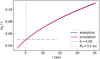 |
Fig. 2 Aspect ratio (i.e., pressure scaleheight scaled with radius) h(r) = Hp(r)/r of our initial set-up. The black dashed line is the analytical calculation according to Eq. (5), the pink solid line shows the Gaussian fit from the initial set-up in our simulation. Gray dotted and dashed lines indicate the reference radius R0 = 5.2 au and the corresponding reference aspect ratio h0 = 0.05, respectively. |
3.1 Untilted reference case
We first modeled the reference case of an untilted disk. We set up a disk with mass Mdisk = 0.02 M⊙ around a Solar-like star with a viscosity of αt = 10−3. The surface density parameter was set to ∑0 = 209.2 g cm−2 with a power law exponent of p = 1. We note that in FARGO3D, the set-up is scalable so that the results also apply to different mass and length scales. The disk ranges from rin = 2.6 au to rout = 26 au. We chose an aspect ratio at R0 of h0 = 0.05, along with a flaring index of ifl = 0.5, and we set the temperature structure accordingly. In Fig. 2, we present the aspect ratio of the initial set-up, with both the analytical calculation according to Eq. (5) (black dashed line) and a fit from our simulation data (pink solid line). For the fit, we used a Gaussian function to fit the vertical density profile at each radius according to:
![$\[\rho(z)=\rho_0 \exp \left(-\frac{z^2}{2 H_{\mathrm{p}}^2}\right),\]$](/articles/aa/full_html/2024/09/aa48660-23/aa48660-23-eq7.png) (7)
(7)
where ρ0 is the midplane density, z the height above the midplane, and Hp the pressure scaleheight of the disk. We note that for simplicity, we used the radial shells of the grid instead of extrapolated cylindrical radii to fit the Gaussian profiles. This means that the fitted (pink) curve is only an approximation, however, it is sufficient for the purpose of double-checking our initial set-up. The parameters we chose, namely, the flaring index of ifl = 0.5, result in a globally isothermal disk.
We ran the tilted disk simulations for 500 orbits at R0 = 5.2 au, which translates to ttot = 6000 yr with one orbit being torbit = 12 yr1. For now, we set the resolution of 80 cells in r-direction with the grid logarithmically spaced in r, 100 cells in azimuthal φ-direction and 40 cells in vertical θ-direction with a range of −25.8° < θ < 25.8°.
From the 3D simulations, we compute the surface density using:
![$\[\Sigma(r)=\int_0^\pi \rho_{\varphi}(r, \theta) r \sin (\theta) ~\mathrm{d} \theta,\]$](/articles/aa/full_html/2024/09/aa48660-23/aa48660-23-eq8.png) (8)
(8)
where ρφ(r, θ) is the azimuthally averaged density of the disk. Figure 3 shows the time evolution of the surface density (top panel) and the inclination (bottom panel), defined as the angle between the angular momentum vector and the z-axis. A detailed description of how we retrieve the inclination can be found in Sec. 3.2.
As expected, the inclination remains zero throughout the whole simulation which means the disk stays aligned to the grid midplane. The surface density stays constant on our timescales, except for some deviations at the grid inner and outer edge, due to the rigid boundary conditions. Because this is merely a reference case, we did not investigate the deviations in detail.
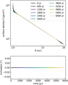 |
Fig. 3 Surface density (top panel) and inclination (bottom panel) evolution of a disk aligned to the grid midplane. The color in the bottom panel highlights the time. The simulation covers a time span of 6000 yr, which are 500 orbits at the reference radius, R0 = 5.2 au. |
3.2 Tilted disk
Next, we tilted the disk by ten degrees with respect to the grid midplane. In a first test, we used the same resolution as in the reference case aligned to the midplane. We set up the tilt in x-direction, meaning that the total angular momentum vector of the disk points in direction of the x-axis, which means a rotation of the disk around the y-axis. Figure 4 shows a cross-section of this set-up.
To retrieve the inclination angle, we determine the total angular momentum vector for each radial shell Lr. To achieve this, we transformed the cell coordinates, as well as the gas velocities, from spherical to Cartesian coordinates. We were then able to calculate the angular momentum vector of each shell using:
![$\[\boldsymbol{L}_r=\int \rho(r, \theta, \phi) \boldsymbol{r} \times \boldsymbol{v} ~r^2 \sin (\theta) \mathrm{d} \theta \mathrm{d} \phi,\]$](/articles/aa/full_html/2024/09/aa48660-23/aa48660-23-eq9.png) (9)
(9)
where υ is the gas velocity. We note that the resulting Lr is given in Cartesian coordinates as well. By normalizing Lr, we get the direction of angular momentum, lr, which we used to compute the inclination angle i using
![$\[i=\arccos \left(\boldsymbol{l} \cdot \boldsymbol{l}_z\right),\]$](/articles/aa/full_html/2024/09/aa48660-23/aa48660-23-eq10.png) (10)
(10)
where lz is the unit vector of the z-axis with (0, 0, 1).
In addition to the inclination, we investigate the precession angle, which we define as the clockwise angle between angular momentum vector projected onto the x-y-plane and the x-axis. This definition gives an initial precession angle of 0°.
Figure 5 shows the surface density evolution, as well as the evolution of inclination and precession angle. The surface density shows a stronger pile-up at the inner boundary and an adjacent density deficit, which we attribute to effects caused by the reflective (rigid) boundary. We investigated this by running two more simulations of the same tilted disk set-up, but using the outflow boundary conditions at the inner edge in radial direction (as shown in Fig. 6). Apart from the boundary condtitons, one simulation has the exact same initial conditions, while the other is set up with an exponential cut-off at the inner and outer disk edges. In this comparison, we indeed see that the pile-up at the inner edge is caused by the rigid boundary conditions and does not occur in the simulations with inner outflow conditions. However, we observe that the inner region of the disk shows a density deficit in comparison to the initial state ranging up to 5 au. Interestingly, this seems to occur in all three simulations, which suggests that this is not an effect caused by the inner boundary. We suspect that this effect could be caused by an unphysical warp that we find in the simulation, which we discuss later in this section. As we are mainly interested in the alignment with the grid, we do not go into more detail here. We merely note that special care should be taken when looking at the surface density evolution of the inner region in our simulations.
In an ideal set-up, the inclination and precession angle should stay constant. In our simulation (Fig. 5), we see that the inclination decreases over time. This means the disk is dragged by numerical effects toward an alignment with the grid geometry. However, considering a total decrease of less than 1.5 degrees over a time span of 6000 yr, the result is surprisingly good.
The precession angle, however, shows a much stronger trend. During the simulated period of 6000 yr, the disk precesses by approximately 75° in a counter-clockwise motion (negative precession angle). Physically, the disk should not precess; therefore, this is clearly an effect caused by the grid. The reason for the effect could be numerical friction a gas particle experiences when traveling from one cell to another. Because the disk is tilted, a gas parcel has to not only travel through all cells in φ-direction within one orbit, but additionally through several layers in θ-direction. This increases the amount of numerical friction and might cause the gas parcel to be slightly delayed in its motion through the θ-layers. Therefore, a gas parcel arrives later at its original θ-height and the whole disk shows a precession motion in the same direction as the orbital rotation; that is, in our simulation, the orbital direction of the disk is counter-clockwise, as well as the precession. This can indeed be explained by a delay in θ: The vertical motion of the gas parcels in a tilted disk during one orbit can be considered like shifting a Gaussian function up and down, similar to an advection. For advection schemes, Icke (1991) investigated the phase-shift P due to numerical friction (see their Eq. (3.10)). For P > 0, the phase is lagging, which means that the transported function is trailing behind the true solution. Icke (1991) found that the investigated higher-order advection schemes resulted in this phase-lag, namely, P > 0. Even though FARGO3D uses a different advection algorithm, it is likely this algorithm has the same problem when the resolution is too low. Our findings agree with this hypothesis, that is, we are able to explain the precession we find in our simulation with a phase-lag caused by numerical friction. Because the numerical friction decreases when the resolution is increased, we expect the precession effect to be reduced in higher resolutions. We describe how we tested this aspect in Sec. 3.3.
In Fig. 5, in addition to the decrease of inclination, we can also observe an oscillation pattern. To investigate its cause, we took a look at the inclination profiles in different time steps. We chose the first and second period from maximum to maximum, which is indicated by the grey dashed lines in Fig. 5, bottom panel. The first period roughly extends from 420 to 1140 yr, the second from 1140 to 1860 yr.
Figure 7 shows the evolution of the inclination profile during these two periods with the time axis as a third dimension, where the color scheme from blue to yellow indicates one period. We find that the inclination profile varies periodically, which can explain the oscillations in the averaged inclination angle for the total disk. We find that the disk is not perfectly planar which would have a constant inclination profile with radius. This means that the disk in our simulation is slightly warped and evolves in a typical wave-like warp evolution. We note that the warping is modest and not caused by a physical effect but results from numerical grid effects. The warp might arise due to the grid effects not having the same strength at all radii. Because the orbital period is shorter at smaller radii, the inner disk experiences more numerical friction than the outer disk in a given time. As this is not a physical effect, we do not further investigate the evolution of the warp. Additionally, it is rather modest and does not strongly interfere with our evaluation of the grid effects. However, it can explain the oscillations in the mean inclination of the total disk. We additionally suspect this to influence the evolution of the surface density, as mentioned earlier in this section.
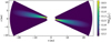 |
Fig. 4 Cross-section through the initial tilted disk along the x-axis. |
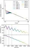 |
Fig. 5 Similar to Fig. 3, but for the a disk tilted by 10° with respect to the grid midplane. The additional panel at the bottom shows the precession angle of the disk. The grey dashed lines indicate the inclination oscillation periods investigated in Fig. 7. |
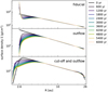 |
Fig. 6 Surface density evolution of a tilted disk by 10° in simulations with different boundary conditions. The top panel shows our fiducial set-up with rigid boundaries, the middle is the same set-up, but with the outflow boundary conditions at the inner edge, and the bottom panel has an exponential cutoff at outer and inner edge, in addition to inner outflow boundary conditions. |
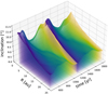 |
Fig. 7 Inclination profile evolution during the first and second periods of the inclination oscillation. Each period is indicated by the color scale from blue to yellow. The first period extends from 420 to 1140 yr, the second from 1140 to 1860 yr. |
Resolutions in different simulations.
3.3 Different resolutions
In this section, we investigate the grid effects in different resolutions. We aim to probe the influence of resolution in the three directions and therefore set up three simulations: one with resolution doubled only in r-direction (we call this simulation r_resolution), a second one with resolution doubled in φ-direction (called phi_resolution), and a third one doubling only the θ resolution (theta_resolution). In a fourth simulation (high_resolution), we used a higher resolution in all three directions: 160 cells in r, 200 cells in φ, and 160 cells in θ. An overview over the simulation resolutions is presented in Table 1, with the differences between the simulations highlighted in orange.
Figure 8 shows the inclination and precession in the simulations with varying resolutions. Looking at the inclination evolution, we find that the decrease of inclination is weakest for the simulation high_resolution: Comparing the three simulations with increase of resolution in one direction each, we find that the grid effects are especially sensitive for resolution in θ-direction. The inclination oscillations become weaker and the overall decrease is less steep. Resolution in the r-direction, however, shows no significant improvements, compared to the fiducial set-up from Sec. 3.2.
We find that resolution in r and φ do not influence the precession motion. However, higher resolution in θ makes a large difference for the precession, as we have already suspected in Sec. 3.2. In simulation theta_resolution, there is almost no precession of the disk. This indeed confirms our suspicion that the precession is mainly caused by friction of gas parcels that have to travel through several θ-layers because of the tilt. We note that simulation high_resolution is slightly precessing in the other direction. However, this precession is still small compared to the fiducial resolution.
Overall, we find that the grid effects get weaker for higher resolution, as expected. The oscillation of the inclination and precession angle we investigated in Fig. 7 becomes much weaker when increasing the θ-resolution. Higher resolution can severely increase the computation time. Doubling the resolution in all three directions prolongs the computation by a factor of 16 (23 = 8 for the three directions and an additional factor of two due to the decreased time step). However, the simulations we are investigating in this work are still feasible, because we can take the advantage of multi-node GPU parallelization. For our purposes, we find the grid effects of simulation theta_resolution to be sufficiently small. Therefore we continued using this resolution for our investigations of a warped disk, described in Sec. 4.
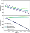 |
Fig. 8 Inclination (top panel) and precession angle (bottom panel) in simulations with varying resolutions in a disk tilted by 10° with respect to the grid midplane. |
3.4 Dependence on viscosity
To investigate the role of viscosity for the grid effects, we perform four further simulations varying the viscosity parameter αt. For these simulations, we use the initial low resolution (see Sec. 3.2). We keep the set-up exactly the same except for the viscosity, which we set to αt = 10−5, αt = 10−4, αt = 10−2, and αt = 10−1. The fiducial simulation investigated in previous sections has a viscosity of αt = 10−3.
Figure 9 shows the evolution of the inclination and the disk precession in those simulations. The simulations with αt = 10−5, αt = 10−4, and αt = 10−3 show a very similar behaviour with almost the same amount of decrease in inclination and precession angle. For higher viscosities, however, the grid effects seem to be much stronger. We investigated the same simulations in higher resolution (corresponding to theta_resolution) and find that the grid effects significantly decrease for all viscosities (dotted lines in Fig. 9). However, the simulation with the highest viscosity, αt = 10−1, still shows slightly stronger numerical effects than the other simulations. This means that in order to accurately model higher viscosities, it is even more important to consider a higher resolution. In this work, we are mainly interested in viscosities of αt = 10−3 and lower and therefore do not go into more detail here. It should, however, be kept in mind for future projects.
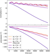 |
Fig. 9 Same as Fig. 8, but for simulations using varying viscosities. The disks are still tilted by 10° with respect to the grid midplane. The dotted lines show the same simulations with higher resolution in θ-direction (corresponding to theta_resolution in Table 1). |
3.5 Higher inclination
In order to study the grid effects for a different tilt inclination, we perform a simulation of a disk tilted by 30° with respect to the grid midplane. For this, we decided to use a higher resolution, namely, it is the same as in simulation high_resolution. Since our disk is more inclined, we need to extend the computation domain in θ-direction. In order to achieve the same resolution in θ for this case, we need more grid cells in θ. Table 2 shows the resolution comparison between the two simulations. We kept the cell amounts in r and φ the same.
Figure 10 shows that the inclination decreases by about two degrees over a time span of 6000 yr. We can roughly estimate the decay rate λ = −1/i di/dt = −2°/30° 1/(6000 yr) to λ = −1.1 × 10⁻⁵ yr−1. When comparing this to the simulation high_resolution with λ = −0.5°/10° 1/(6000 yr) = −8.3 × 10⁻⁶ yr−1, we see that the decay rate for higher inclinations is higher. We therefore expect the inclination decay not to be perfectly linear. For future projects investigating higher inclinations, we keep in mind that more tests should be made. The precession of the disk varies a little, but the change stays within a few degrees.
All in all, we find that the grid effects can be negligible for a high enough resolution. The resolution we find is still feasible for full 3D hydrodynamic simulations. We therefore conclude that it is possible to simulate disks with out-of-plane features using a grid-based method, when keeping in mind that grid effects might play a role under certain conditions.
Resolution comparison between different inclinations.
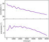 |
Fig. 10 Inclination (top panel) and precession (bottom panel) evolution of a disk tilted by 30° with respect to the grid midplane. |
4 Warped disk
To investigate the warp evolution in 3D hydrodynamics, we set up an initially warped disk around a single central star. We note that the shape of the warp is not physically motivated by any formation scenario, as we are interested in the evolution from that point on. The initial warp is given in Eq. (6). Since we did not include a misaligned binary or companion or any other external component, the warp is not driven and will smooth out according to the warp evolution. The initial maximum warp is imax = 10°. We locate the warp to rwarp = 10.4 au with a width of rwidth = 2.6 au. For the resolution, we chose 80 cells in r, 100 cells in φ, and 134 cells in θ with an extend of −43° < θ < 43°, which keeps the cells-per-scaleheight ratio the same (i.e., 4.4 cps at r = 5.2 au) as in the simulation theta_resolution in Sect. 3.2. We chose this to keep the computational time short so we can perform multiple simulations. We performed one high-resolution simulation doubling the resolution in all three directions and find that the qualitative results are the same. Our evaluation of this high resolution simulation can be found in Appendix A.
Figure 11 shows a cross-section of this initial set-up. Except for the warping of the disk, all parameters are the same as in our previous simulations (see Sect. 3.1). We again chose a turbulence parameter of αt = 10−3 and therefore expected a wave-like evolution of the warp, as h > αt. In the following sections, we investigate the evolution of the inclination profile, as well as the precession profile (=twist) of the disk. We expected the profiles to depend on the radius, therefore, we do not consider at the radially averaged inclination and precession angle.
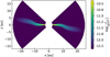 |
Fig. 11 Cross-section of the initial warped disk along the x-axis. |
 |
Fig. 12 Evolution of the inclination profile in the warped disk simulation. The color simply highlights the time. |
4.1 Inclination profile
We first investigated the evolution of the inclination profile in detail. In Fig. 12, we show its evolution. In this figure, the wavelike behavior is evident and is visible as a standing wave of the global bending modes superimposed on a global mean tilt of the disk. This mean tilt of the disk does not visibly decay, although we expect it to decay slowly due to numerical effects. The warp amplitude is dampened over time. Over the first 6000 yr (500 orbits at R0), the disk does not reach the planar state.
To investigate the damping of the warp, we continued running the simulation up to 2.4 × 10⁴ yr (2000 orbits at R0). Figure 13 shows this long-term evolution. The warp is dampened so that we end up with a nearly planar, but spatially tilted disk.
In Fig. 14, we investigate the warp wave period and inclination damping in more detail. We chose a radius close to the outer edge of the disk at r = 22.5 au and fit the inclination evolution at this point with an exponentially decaying cosine function of the form:
![$\[f(t)=A \cos (\omega t-b) \cdot \exp (-\lambda t)+c+d \cdot t,\]$](/articles/aa/full_html/2024/09/aa48660-23/aa48660-23-eq11.png) (11)
(11)
with amplitude parameter, A, frequency, ω, and decay rate, λ. We allow for a phase shift, b, in the cosine function, an offset c, and a linear damping in overall inclination with d.
Our fit gives a wave frequency of ω = 0.008 yr−1, which leads to a warp wave period of
![$\[P=\frac{2 \pi}{\omega}=757 ~\mathrm{yr}.\]$](/articles/aa/full_html/2024/09/aa48660-23/aa48660-23-eq12.png) (12)
(12)
We can make an estimate of the period from linear theory in the following way. The wave speed of the warp wave is approximately half the sound speed in the disk υw = cs/2 (Lubow & Ogilvie 2000). Because we are investigating a globally isothermal set-up for now, the sound speed is cs = 653 m/s everywhere in the disk. We find that the warp wave behaves similarly to a standing wave, with a wave length of twice our radial disk regime λw = 2Δr = 44.8 au. The estimated period then is
![$\[P_{\text {linear theory }}=\frac{\lambda_{\mathrm{w}}}{v_{\mathrm{w}}}=\frac{2 \Delta r}{2 c_{\mathrm{s}}}=657 ~\mathrm{yr} \text {. }\]$](/articles/aa/full_html/2024/09/aa48660-23/aa48660-23-eq13.png) (13)
(13)
We note that this is the same as the sound-crossing time ts = Δr/cs. This means that the period in our simulation is in agreement with linear theory.
In our fit, we find a decay rate of λ = 8.9 × 10⁻⁵ yr−1, which results in a mean lifetime of the warp of τ = 1/λ = 1.1 × 10⁴ yr. Linear theory gives a rough estimate of the warp damping timescale with τlinear theory = 1/(αΩ) with Ω as Keplerian frequency. (see e.g., Nixon & King 2016). If we choose the Keplerian frequency at the outer edge of our disk, this results in τlinear theory = 2.1 × 10⁴ yr, which agrees within a factor of 2 with the findings in our simulation.
From our fit, we also get the mean tilt of the disk (c in Eq. (11)) at our chosen radius, which is 7.7°, and the damping of inclination d, which we find to be −3 × 10⁻⁵ yr−1, which gives a total inclination loss over the simulated 2.4 × 10⁴ yr of 0.74°. This loss of mean inclination is a numerical effect as also found in Sec. 3.2. It is also interesting to note the amplitude from the fit, with A = 1.6°.
We went on to compare the 3D hydrodynamic simulations to a 1D model of warped disks. For the 1D model, we split the disk into concentric annuli and assign each annulus an angular momentum vector that determines the orbital plane of the annulus. This way, we have a 1D parametrization for a 3D object. The angular momentum vector can be updated using Eqs. (1)–(3). We set up the parameters in the 1D model the same parameters as in the 3D model. For this, we use our 1D warped disk evolution code dwarpy (Kimmig et al. in prep.).
In Fig. 15, we find a good agreement between 3D and 1D simulations on short timescales. On longer timescales, however, the 1D model shows a more complicated behaviour than the 3D simulation, as shown in Fig. 16. This might be due to boundary conditions, as we used rigid boundaries in the 3D simulation and open boundaries in the 1D model, as dwarpy is primarily tested with these conditions. There, we chose open conditions in order to avoid a torque from the boundaries acting on the disk. However, the wave-like nature of the inclination evolution is still apparent in the 1D model.
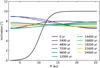 |
Fig. 13 Long-term evolution of the inclination profile in the warped disk simulation. |
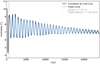 |
Fig. 14 Decay of inclination in the warped disk simulation. We chose to evaluate the inclination close to the outer edge at a radius of 22.5 au. The black line shows the simulation data, the blue dashed line the fit. The grey dashed line indicates the starting point of the fit. |
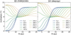 |
Fig. 15 Inclination evolution of the warped disk in comparison between the 3D set-up in FARGO3D (left panel) and the 1D set-up in dwarpy (right panel). For comparability, we plot until 240 yr of simulated time. Note that the computational domain of the 1D simulation is well beyond the outer edge of the figure. |
4.2 Twisting of the disk
In our 3D simulation, we notice a precession motion within the disk, which does not occur in the 1D model for the wave-like regime. The 3D disk shows a differential precession, meaning that the disk precesses differently depending on the radius, which we call a twist. In this section, we investigate the twist in more detail. We aim to find out whether the twist is caused by numerical or physical effects.
At first, we look at the total angular momentum of the disk. We find that its absolute value decreases about 0.5% in the time span of 6000 yr and 2% in the time span of 2.4 × 10⁴ yr. Evaluating the total angular momentum of the planar reference case from Sec. 3.1, we find that the planar disk’s absolute angular momentum also decreases by about 0.5% in the time span of 6000 yr.
Figure 17 shows that the direction of the total angular momentum vector slightly changes over a time span of 2.4 × 10⁴ yr, which are 2000 orbits at R0. The angle between the vectors at the beginning and the end of the simulation is 4.6°. We suspect that the change in direction occurs due to numerical effects. While FARGO3D is programmed such that it conserves azimuthal angular momentum to machine precision, this mainly applies to components perfectly aligned with the grid geometry. We suspect the change in angular momentum we observe in Fig. 17 to be caused by the fact that the numerical scheme does not account for tilted motions. On a timescale of 6000 yr (inclination evolution in this time span plotted in Fig. 12), on which we find a significant twisting of the disk, we find the angular momentum vector to change on an angle of only 1.2°. Notably, the total angular momentum vector does not show any oscillatory behaviour. In spite of the slight changes in angular momentum, we can argue that the changes are small and, therefore, the total angular momentum is reasonably well conserved, both in direction and in absolute value.
We plot the twist of the disk by showing the evolution of the unit angular momentum vectors at different radii in Fig. 18. The angular momentum vectors are extracted from the 3D simulation using Eq. (9).
A twist occurs when the unit angular momentum vectors point in different directions. In the top row of Fig. 18, we show the time evolution of the vectors close to the inner disk edge (left) and close to the outer edge (right). We intentionally did not choose the exact disk edges to avoid potential boundary effects. The disk quickly twists and, after some time, the vectors precess in almost perfect circles.
To investigate this motion more closely, we chose a point in time (300 orbits at R0) at which the circles are already developed and plot in the middle row one and a half periods from that point on. Here, we only plot the x- and y-component of the unit angular momentum vector lr. We find the period to be roughly 60 orbits. We see that both the inner and the outer part precess clockwise. However, because the total angular momentum is conserved in direction (as seen in Fig. 17), the directions counteract, which means that whenever the inner part of the disk points in positive x- and/or y-direction, the outer part points correspondingly in negative x- and/or y-direction. To see this, we indicate a few corresponding times with the symbols in the plot.
In the bottom panel of Fig. 18, we then plot more radial points in the disk, each radius in a different color. We note that we offset the twist for each radius by a factor of r/(60 au) in order to disentangle the circles. We chose a linear spacing for the radial evaluation points. At all radii, the disk precesses clockwise, and the counteracting of the directions can be seen in this plot in more detail. One part of the disk always counteracts the precession of another part, so that the total angular momentum is conserved. A clearly twisted state of the disk occurs for example in the snapshot at 308 orbits, which is illustrated with grey stars.
We note that in the long-term evolution of the system, the precession is dampened. This happens on the same timescale as the inclination of the warp is dampened. Additionally, the precession period of the vectors coincides with the inclination wave period.
To explore the origin of the disk’s twist – whether it is a numerical or physical effect – we conducted a series of tests, which can be found in Appendix B, and we briefly summarize: The fact that the total angular momentum does not exhibit any oscillatory motion led us to rule out the inner and outer grid boundary as a cause for the twist. To investigate further, we performed a new simulation, pushing the outer boundary far away from the physical grid edge by applying an exponential cut-off to the disk density. In this scenario, the outer boundary is unlikely to influence the physical outer edge of the disk. However, even in this case, the twist persisted. Furthermore, we performed 1D simulations to explore if the twist might be triggered by the initial conditions in the 3D simulation. However, the 1D model failed to reproduce the twist observed in the 3D model. This strongly suggests that the twist is indeed a 3D phenomenon. Interestingly, a similar effect can be seen in SPH simulations of warped disks (Martin, priv. comm.).
While we cannot be completely sure at this point, our tests indicate that the twist likely arises from a physical cause rather than being a numerical artefact. We suspect that specific terms neglected in the linearization process in deriving the 1D equations play a role in why the 1D model cannot reproduce the twist.
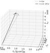 |
Fig. 17 Direction of the total angular momentum vector in the beginning of the simulation t = 0 yr (grey dashed line) and in the end t = 2.4 × 10⁴ yr (solid black line). The line connecting the two arrows indicates the time evolution with darker color the later the time. |
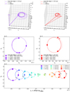 |
Fig. 18 Twist motion in the warped disk simulation. Top row: unit angular momentum vectors close to the inner (left panel) and outer (right panel) edge of the disk for the first t = 6000 yr. Similar to Fig. 17. Middle row: x-y components of the unit angular momentum vector at the same radii as in the top row, but only for the time period between 300 and 390 orbits at R0, chosen to roughly show 1.5 precession periods. The direction of the precession is indicated by the arrows. x-markers show the beginning of the plotted time, squares the end. Diamonds indicate the middle of this time period (45 orbits after the x-markers). Bottom row: same as middle row, but for various radii, plotted with an offset of r/(60 au) in y-direction to disentangle the twist at different radii. The stars show the lx−ly components at a snapshot at t = 3696 yr (308 orbits at R0), which shows a twisted state in the time evolution. |
4.3 Investigating a differently flared disk
In order to relax the assumption of a globally isothermal disk, we ran an additionally simulation with a locally isothermal disk using a flaring index of ifl = 0.25 (see Eq. (5)) and setting the temperature structure accordingly. We keep all other parameters the same. A cross-section of the initial set-up is shown in Fig. 19.
Investigating the inclination evolution, we find the expected wave-like behavior, as shown in Fig. 20.
The overall behavior is similar to the globally isothermal disk. However, there seems to be an amplitude modulation with a period of about 4000 yr, which can also be seen when we look at the inclination evolution at a specific radius (we chose r = 22.5 au) as shown in Fig. 21 (black line). This could be either a numerical or a physical effect, which would require further investigation. This would go beyond the scope of this work, thus we simply mention this observation at this point.
In Fig. 21, we investigate the inclination decay rate according to Eq. (11) and find a decay rate of λ = 1.3 × 10⁻⁴ yr−1, which gives a mean lifetime of τ = 1/λ = 7.7 × 10³ yr. This is slightly shorter than the fitted mean lifetime of the globally isothermal disk. For reference, linear theory gives an estimation of τlinear theory = 1/(αΩ) = 2 × 10⁴ yr, which does not depend on the disk’s vertical structure. In future work, the influence of the vertical structure on the warp lifetime could be investigated in more detail.
In Appendix B, we investigate the twist of the locally isothermal disk. We find that it still occurs, but the twist behavior appears to be more complicated than in the globally isothermal case.
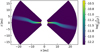 |
Fig. 19 Cross-section along the x-axis of the locally isothermal warped disk. |
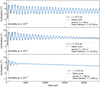 |
Fig. 22 Inclination evolution at radius r = 22.5 au (black solid lines) in simulations with different disk viscosities. The blue dashed lines indicate the fit according to Eq. (11). The middle panel corresponds to the fiducial simulation and is the same as Fig. 14. |
4.4 Different viscosities
We further test the dependence of the warp and twist on viscosity and perform two additional simulations, using the same initial set-up but varying the original αt = 10−3 to lower (αt = 10−5) and higher viscosity (αt = 10−2).
We plot the inclination evolution at a radius r = 22.5 au (close to the outer edge) of the simulations with varying viscosities in Fig. 22 to investigate the warp decay rates. We find that for a ten times higher viscosity (bottom panel), the warp is dampened roughly 10 times faster than in our fiducial simulation, as expected by linear theory (recall τlinear theory = 1/(αΩ)). For the low viscosity simulation (top panel), the mean lifetime is longer than the fiducial simulation, as expected. However, instead of the factor 100 predicted by linear theory, we find a factor of roughly 4. This could mean that the simulation is influenced by numerical viscosity and grid effects, or that additional effects play a role in dampening the warp that are not taken into account in the derivation of the timescale estimation. Investigating the reason here in detail would go beyond the scope of this work.
In Fig. 23, we plot the precession angle over time for the three different viscosities. Recall that we define the precession angle as the clockwise angle between x-axis and angular momentum vector projected onto the x-y-plane, giving an initial precession angle of 0° at all radii. We plot the precession angle at different radii (colored lines). As a reference, we additionally plot the precession angle of the total angular momentum vector (black dashed line) and note that it does not oscillate.
In all cases, we find that the total angular momentum vector changes direction in time, which means that the disk overall precesses. This overall precession is more pronounced in the high viscosity case, α = 10−2. This is not a physical effect, but a result from grid effects, as explored in Sec. 3.4. A higher resolution would help keep the direction of the angular momentum conserved for a longer time period. However, since we were mainly interested in the differential precession, namely, the twist, we did not perform additional simulations in higher resolution at this point.
In all cases, we found a twist, which is dampened much faster for high viscosity. The precession period is similar for all viscosities, as indicated with the grey dotted lines in Fig. 23, and roughly equals 740 yr. Despite the fact that parts of the disk clearly precess, the total angular momentum direction does not oscillate. We take this as another indication that the twisting behaviour is physical, although the reason for it is not clear yet.
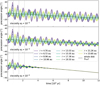 |
Fig. 23 Precession angles for different radii (colored lines) in simulations with different disk viscosities. The black dashed line in each panel shows the precession angle of the angular momentum vector, Ltot, of the whole disk. The grey dotted lines indicate precession periods of roughly 740 yr. |
5 Internal dynamics of the warped disk and origin of the torques
5.1 Sloshing motions and internal torques
The internal torque responsible for the propagation of a warp through the disk is primarily due to resonant horizontal internal gas motions (Papaloizou & Pringle 1983; Papaloizou & Lin 1995; Lubow & Ogilvie 2000). We refer to these as “sloshing motions” because they are caused by sideways pressure gradients due to the warp (see Fig. 5 of Ogilvie & Latter 2013a), and behave very similar to a layer of water on a tilted tray. For any snapshot of a 3D warped disk model, the internal torque can be calculated as shown in Appendix C.
A description of how these internal sloshing motions are driven, how they behave, and how they give rise to an internal torque, was given in DKZ22. There, the authors used a variant of the local shearing box approach of Ogilvie & Latter (2013a). After employing two linearization steps, they derived the solutions for the sloshing motions, and from those obtained a generalized set of 1D warped disk equations. With our 3D model, we can investigate how good these approximate solutions for the sloshing motions are, as we can directly analyze the motions of the gas inside the 3D disk and compare them to the predictions of DKZ22.
Of course, we are not the first to compare 3D warped disk models to 1D models. For instance, Nelson & Papaloizou (1999) performed 3D SPH simulations of warped disks in both the wavelike and diffusive regime, and compared the results to 1D models. They also see the sloshing motions in their 3D models. In our FARGO3D model in spherical coordinates, we have the advantage compared to SPH models that we can study the disk many scale heights above the midplane, where the densities are orders of magnitude lower than at the midplane. While these regions do not contribute significantly to the internal torque, they may contribute to observations of the disk.
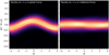 |
Fig. 24 Gas density of the disk annulus at r = 8.3 au at time t = 120 yr. The map is a standard (ϕ, θ) projection of the sphere of constant distance to the star. The color scale is linear. Left: in unrotated coordinates. Right: in rotated coordinates such that the disk annulus lies in the equatorial plane. |
5.2 Sloshing and breathing motions in the 3D model
To compare the internal dynamics of our 3D warped disk model with the local shearing box approach of DKZ22, we chose a single annulus of the disk, namely, we chose a radius, r, at which we performed the comparison. In DKZ22, the global disk is assumed to be oriented such that the l vector (the unit vector perpendicular to the disk annulus) at this radius points into the global positive z-direction (see Fig. 2 of DKZ22). Furthermore, the disk is oriented such that the local warp vector ψ = dl/d ln r points in the positive x-direction. To compare our 3D disk model, at radius r, with the local shearing box description of DKZ22, we therefore need to rotate it to this configuration.
There is, however, a small numerical subtlety. The first rotation, putting l into the positive z-direction, is a straightforward rotation around the l × ez axis, where ez is the unit vector in the global z-direction. In our 3D model we perform this rotation as a coordinate mapping using linear interpolation, and, of course, we also rotate the velocity vectors accordingly. The second rotation, however, which is the rotation around the z-axis such that ψ points into positive x-direction, can cause numerical difficulties. This is because numerical noise can make the direction of the warp vector ψ wiggle wildly at radii for which |ψ| ≪ 1; for instance, around radii where it flips sign. As long as we only study a single annulus of the disk this is not a problem. However, when comparing the results of neighbouring annuli, we might find major differences simply due to large differences in horizontal (x-y) orientation. This is purely an artefact of the choice of horizontal orientation. Since our disk model is initiated with a warp purely in the x-z-plane, we chose, for this section, to omit the second rotation. The global orientation of the model is close enough to the DKZ22 choice that we can perform our analysis.
We analyzed our model at time of t = 120 yr (10 orbits at R0) at a radius of r = 8.3 au. We chose this point in time because the disk already had some time to relax and the internal torques are fully developed, but the disk system did not have time yet to change much. At this moment, this disk annulus is inclined with respect to the coordinate system by −3.8°. If we display the density in the unrotated angular coordinates θ, ϕ, this leads to the image Fig. 24-left, where the annulus looks wavy. If we remap this into a new, rotated, coordinate system, the disk annulus becomes straight (Fig. 24-right). We can see that the density at the disk midplane has moderate maxima and minima. They are caused by the vertical expansion and compression motion, called “breathing motion” by Ogilvie & Latter (2013a).
In this new rotated frame, we can analyze the radial velocity υr(θ, ϕ), namely, the sloshing motion, and the vertical velocity υz(θ, ϕ), namely, the breathing motion. These are shown in Fig. 25. The Keplerian motion of the gas flows from left to right (toward increasing ϕ), which can therefore be regarded as kind of a time axis, even though these figures show one snapshot in time. In the left panel it can be seen that, as expected, the radial velocity υr(z, ϕ) has consistently opposite sign above/below the disk midplane. This is the sloshing motion that produces the internal torque. Far from the midplane, this sloshing motion becomes supersonic. However, most of the torque is produced below about one scale height (root-mean-square height of the disk above the disk’s midplane); that is, the grey dot-dashed line in the figure, where the motions are subsonic, so that the torque is presumably not much affected by the supersonic motions higher up. The grey lines in Fig. 25 mark the vertical extend of the disk, that is, the root-mean-square widths of the vertical Gaussian density profile. The lines become slightly wavy due to the breathing motion causing the vertical compression and expansion in the disk.
The right panel shows the vertical motion of the gas. In this figure, the sign flips at the disk midplane as well, meaning that the motion is either expanding or compressing the disk vertically (i.e., the breathing motions). These motions are much weaker than the sideways sloshing motions, but they also become supersonic far above the disk midplane, leading to the formation of shocks where the upward (blue) motion hits the downward (red) motion.
These results show that the sloshing and breathing motions predicted from the linearized shearing box model (Ogilvie & Latter 2013a, DKZ22) are indeed occurring in the 3D warped disk model. And these velocities can be quite large, close to or exceeding the sound speed, especially at two or more scale heights above the disk surface. This may have relevant consequences for kinematic observations (using molecular lines) of warped protoplanetary disks.
In Fig. 26 we show a vertical slice of Fig. 25-left, at azimuth ϕ = 1.29. The figure shows that the linear approximation of the sloshing motion υr(r, z, t) = Vr(r, t)Ωz, which stands at the basis of all 1D warped disk models, appears to be a good approximation up to several scale heights at this radius and time. Deviations do occur at some other radii and times, but overall they are minor.
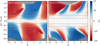 |
Fig. 25 Gas velocity components in units of the local isothermal sound speed at r = 8.3 au at time t = 120 yr, in the rotated frame (as in Fig. 24-right). The colors are linear between −1 and 1, and logarithmic for |υ/cs| > 1. Note: the isothermal sound speed cs is constant at 0.66 kms−1 throughout each panel, consistent with a disk aspect ratio of hp/r = 0.064. Left: Radial velocity (sloshing motion). Right: Vertical velocity (breathing motion). The dot-dashed, dashed and dotted grey lines mark the rms vertical extend of the disk (which would relate to the pressure scale height in a steady-state disk), twice that, and three times that. The grey areas below and above are the regions outside the model grid. |
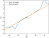 |
Fig. 26 Radial gas velocity in units of the local isothermal sound speed, at the same radius and time as in Fig. 25, at azimuth ϕ = 1.29, i.e., a vertical slice of that figure. The blue curve shows the data from the 3D model, the orange curve a linear reconstruction using a slope computed as in Appendix D. |
6 Conclusion
We performed 3D simulations of misaligned disks using FARGO3D (Benítez-Llambay & Masset 2016). To study the applicability of the grid-based code to misaligned features, we set up a disk that is planar, but tilted with respect to the grid midplane and compared the result to a planar disk aligned to the grid midplane. The latter case has been studied extensively in previous works, therefore, we used it as our reference case. Physically, the tilted case should lead to the same results, meaning all deviations in the simulation result from grid effects, namely, numerical friction. We find that grid-based methods can simulate misaligned features surprisingly well, given a high enough resolution. We find the vertical resolution (in θ) to be most important in terms of avoiding grid effects. Additionally, the minimum required resolution to accurately model misaligned features depends on disk viscosity: for higher viscosity, a higher resolution is needed. For future studies using high viscosities in grid-based methods, we recommend performing resolution studies in these specific cases.
We set up an initially warped disk around a single star and we did not include any component driving the warp. Evaluating the warp evolution in this isolated system, we find the evolution to take on a wave-like character, as expected. Comparing the evolution to a 1D ring code model, we find good agreement in inclination evolution. Looking at the twist of the disk, however, we find a significant twisting in the 3D model, which is not seen in the 1D model. The absence of this effect in the 1D model does not necessarily mean that it is an unphysical effect. Looking at the total angular momentum of the whole disk, it does not precess and, in fact, is conserved in both absolute value and direction, which indicates the twist not to be caused by grid effects. Further tests, including a comparison to 1D models and decreasing the importance of the outer boundary by moving it away from the disk edge point to the same conclusion. For higher viscosity, we observe a less pronounced twisting with a faster damping of the precession motion. We suspect the twist to be a physical effect in the 3D warp evolution. The reason why it is not seen in 1D models could be that the effect was neglected in the linearization process.
Evaluating the internal dynamics in our simulation in detail, we find a sloshing and breathing motion, as predicted in the local shearing box approach in DKZ22. These motions are mainly responsible for the warp evolution and lead to the generation of the internal torque. We find that the sloshing and breathing velocities can become supersonic in the upper layers of the disk. Although the upper layers do not significantly influence the warp evolution, since the internal torque is produced close to the midplane, it may have a significant influence on kinematic observations of warped disks.
Acknowledgements
We kindly thank Philipp Weber and Thomas Rometsch for their help in using FARGO3D and the bwForCluster BinAC, inspiration of plots, and comments on the project. We thank Rebecca Martin for helpful discussions. We further thank Hubert Klahr and Ralf Klessen for discussions and helpful comments. We remember the legacy of Prof. Willy Kley, who passed away in 2021, and would have been a part of this work. Additionally, we thank the referee for very helpful comments and suggestions. We acknowledge funding from the DFG research group FOR 2634 “Planet Formation Witnesses and Probes: Transition Disks” under grant DU 414/23-2 and KL 650/29-1, 650/29-2, 650/30-1. Additionally, we acknowledge support by the High Performance and Cloud Computing Group at the Zentrum für Datenverarbeitung of the University of Tübingen, the state of Baden-Württemberg through bwHPC and the German Research Foundation (DFG) through grant INST 37/935-1 FUGG. We gained great benefit for this work from Core2disk-III, which is supported by the LABEX P2IO, the PCMI, PNPS, and PNP programs, and the OSU Paris-Saclay. Plots in this paper were made with the Python (Van Rossum & Drake 2009) library matplotlib (Hunter 2007). We acknowledge also the usage of numpy (Harris et al. 2020), scipy (Virtanen et al. 2020), and astropy (Astropy Collaboration 2022).
Appendix A High-resolution simulation of a warped disk
To check the dependency on resolution, we performed a simulation of our fiducial warped disk set-up with a higher resolution. For this simulation, we doubled the resolution in all three directions, which means 160 cells in r-direction (3.4 cells-perscaleheight at r = 5.2 au), 200 cells in ϕ-direction (1.6 cps at r = 5.2 au), and 264 cells2 (8.2 cps at r = 5.2 au) in θ-direction.
 |
Fig. A.1 Evolution of the inclination profile in the high-resolution warped disk simulation. The color highlights the time. Similar to Figure 12. |
Figure A.1 shows the wave-like behavior of the simulation. Like in the simulation with lower resolution, we see a global bending mode superimposed on a global tilt. The bending mode appears as standing wave with a wavelength of twice the radial disk regime.
To evaluate the bending mode in detail, we fit the inclination evolution in the outer part of the disk (i.e., at r = 22.5 au) with Equation 11 (see Figure A.2). The fit parameters give an amplitude A = 1.6°, a frequency of ω = 0.0083 yr−1, a decay rate of λ = 6.8 × 10⁻⁵ yr−1, a global tilt of c = 7.7°, and a global (numerical) inclination loss of d = −6.8 × 10⁻⁶ yr−1. These parameters indicate a period of P = 750 yr and a mean lifetime of τ = 1.5 × 10⁴ yr.
In comparison to the fiducial resolution simulation, we find a slightly shorter wave period and a slightly lower decay rate leading to a slightly longer mean lifetime of the warp. However, the difference is small (much lower than one order of magnitude) and we can therefore say that the two simulations are in good agreement with each other. Unsurprisingly, we find a much lower inclination loss, d, by one order of magnitude, which supports our assumption that these differences are caused by numerical effects.
Additionally, we briefly evaluate the twisting of the disk in the high resolution simulation, see Figure A.3. For the plot, we chose the same time intervals as for the fiducial resolution. The twisting behavior of the disk stays the same and does not seem to be strongly influenced by resolution.
Figure A.4 shows the evolution of the precession angles at different radii, as well as the overall precession of the disk in both the fiducial and high resolution simulations. The comparison clearly shows that the overall precession of the whole system (negative slope of the black dashed line for the fiducial resolution) is an effect caused by numerical effects, as it does not decrease significantly in the high resolution simulation. The twisting motion, however, is very similar in both simulations, suggesting that it is not caused by numerical effects due to too low resolution. The estimated period of the twisting motion of roughly 740 yr (grey dotted lines) coincides with the fitted period of inclination evolution.
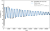 |
Fig. A.2 Decay of inclination in the high resolution warped disk simulation. We evaluate the inclination at r = 22.5 au. The black line shows the simulation data, the blue dashed line shows the fit. The grey dashed line indicates the starting point of the fit. Similar to Figure 14 (note the slightly shorter simulation time). |
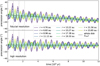 |
Fig. A.4 Precession angles for different radii (colored lines) in simulations with different resolutions. The black dashed line in each panel shows the precession angle of the angular momentum vector Ltot of the whole disk. The grey dotted lines indicate precession periods of roughly 740 yr. Similar to Figure 23. |
Appendix B Investigation the disk twist
In this section, we describe several tests we carried out to investigate whether the twist we found in the warped disk simulation is a numerical or a physical effect.
B.1 Outer boundary
We first performed another 3D simulation where the outer boundary is far away from the disk edge by applying an exponential cut-off to the density profile. In this case, the grid edge is unlikely to influence the simulation.
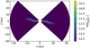 |
Fig. B.1 Set-up of a warped disk with the outer boundary further away from the physical disk edge. |
Figure B.1 shows the initial set-up of this simulation. We keep the same initial conditions as in the previous simulation of the warped disk, the only difference being the cut-off at r = 26 au in the density profile. As we enlarge the radial space of the grid, we keep the number of cells in the disk domain (within 26 au) the same.
 |
Fig. B.2 Twist of a disk with the outer boundary far away from the disk edge, like Figure 18, bottom panel. |
Figure B.2 shows that we also find twisting of the disk. However, the frequency is on a longer timescale than before. Evaluating the inclination evolution of the disk in this set-up, we find that it also takes place on longer timescales, namely, that the warp wave takes longer to travel through the disk. Again, the timescale of the inclination wave corresponds with the timescale of the twist frequency. We find the reason for this to be the cutoff smoothing out on relatively short timescales, as shown in Figure B.3. This leads to the disk being slightly larger, therefore, the timescale of the warp wave is longer. We suspect the reason for this to lie in our initial set-up of the azimuthal velocity, as the smooth-out occurs very quickly. In future work, this could be improved by accounting for the density gradients in the initial set-up.
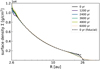 |
Fig. B.3 Surface density of a disk with the outer boundary far away from the disk edge (solid lines). The initial state of the fiducial simulation is plotted as reference (dashed line). |
However, the outer boundary is still unlikely to influence the outer disk edge in this simulation, because the density is very low outside of 26 au. The fact that the twisting persists is an indication that the twist results from a physical process in a warped disk.
B.2 1D models
To rule out the notion that the twist is an effect kicked off some time in the beginning of the 3D simulation, we investigated the behaviour of a twist in a 1D model. For this purpose, we take the twisted state at 308 orbits at R0, which is t = 3696 yr and use it as initial condition for a 1D simulation using our code dwarpy (Kimmig et al., in prep).
We performed two simulations using this state of the warp. In the first simulation, we used the internal torque extracted from the 3D simulation (see Appendix C). To evaluate the difference it makes, we performed another simulation setting the internal torque values initially to zero and let the 1D equations take care of its evolution. The first case (with extracted internal torque) is shown in Figure B.4, top panel, the latter case (internal torque set to zero) in the bottom panel. In both panels, the stars show the initial state of the unit angular momentum vectors (same as the grey stars in the bottom panel of Figure 18). The squares show the state at the end of our simulation time span, which we chose to be the same as plotted in Figure 18.
We find that the 1D model fails to recreate the circular motion of the unit angular momentum vectors. The simulation with the initial torque set to zero (bottom panel of Figure 18) shows no circular motion at all, while the simulation with internal torque extracted from the 3D simulations shows deformed ellipses. The latter is the more self-consistent one, which shows a hint of the circular twist motion, but cannot reproduce the full twist seen in the 3D simulation.
From this, we can say that the twisting of the disk seems to be a 3D effect that is not captured in the 1D equations. It might be an effect traced by linear or non-linear terms that were neglected in deriving the equations. We can conclude here that the twist is an effect triggered continuously in the 3D simulation, as opposed to an event kicked-off once.
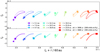 |
Fig. B.4 Evolution of the twisted state in a 1D simulation using dwarpy in two different simulations. The initial state of the warp in both simulations is taken from the twisted state in the 3D simulation at t = 3696 yr (308 orbits at R0). The top panel shows the 1D simulation with internal torque G extracted from the 3D simulation, the bottom panel shows the same simulation, but internal torque G initially set to zero for comparison. Details comparable to Figure 18 (bottom panel). |
B.3 Keplerianity of the warped disk
In 1D models, an untwisted and perfectly Keplerian disk will not twist. However, if the disk deviates from Keplerianity, a twist can be triggered (second term on left hand side of Equation 3). We therefore took a closer look at the azimuthal velocity of the warped disk in the 3D model. Because the orbital plane does not always align with the grid plane, the evaluation of the azimuthal velocity is not straight forward: we need to perform an interpolation. For the interpolation, we use the unit angular momentum vector determining the orbital plane of each grid shell and use the LinearNDInterpolator function from scipy (Virtanen et al. 2020). This way, we can extract the azimuthal velocity of the disk midplane in each grid shell.
Figure B.5 shows that the azimuthal velocity of the disk deviates from the Kepler velocity as we set up the disk with pressure correction terms. During the simulation, we do not observe strong deviations from our initial set-up, except at the inner and outer boundaries, which means that the warp does not significantly change the azimuthal velocity. The deviation from Keplerian motion results from pressure correction in the initial set-up of the disk. Because the deviation is small, we do not expect this to be the sole reason for the twist. In a future work, this could be investigated using 1D models with an adjusted apsidal frequency.
B.4 Twist of a differently flared disk
In this section, we investigate the twist behavior of a locally isothermal disk with a flaring index of ifl = 0.25, as described in Section 4.3.
Figure B.6 shows the evolution of the unit angular momentum vectors. The top row indicates the time evolution of the vectors. We clearly see that a twist develops in the disk. However, the behavior looks more complicated than in the globally isothermal case (see Figure 18). We find that instead of circles, the precession motion takes on an oval or crescent shape, whose orientation also precesses. In the bottom panel, we plot the same time period as plotted in Figure 18 in order to see the oval shape of the twisting motion more clearly.
 |
Fig. B.5 Azimuthal velocity (top panel) and the residuals from the Kepler velocity (bottom panel). The black dashed line shows the Kepler velocity. |
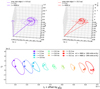 |
Fig. B.6 Twist motion in the locally isothermal disk. Top: Unit angular momentum vectors close to the inner (left panel) and outer (right panel) edge of the disk for the first t = 6000 yr. Bottom: x-y-components of the unit angular momentum vector for the time period between 300–390 orbits at R0 at varying radii, plotted with an offset of r/(60 au) in y-direction to disentangle the twist at different radii. The x-markers show the beginning of the plotted time, the squares the end. Similar to Figure 18. |
We additionally checked the evolution of the total angular momentum vector in the locally isothermal case. Just like in the globally isothermal case, we find very little loss of absolute value (0.67% within 2.4 × 10⁴ yr) and a slight change in direction (4.2° within 2.4 × 10⁴ yr), which we suspect to occur due to the nonconservative nature of the code for out-of-plane features. Most importantly, we also do not see any precession behavior of the total angular momentum vector, which means that the twist in the locally isothermal case is also conserving the total angular momentum within the disk.
We take the fact that a twist also occurs in a differently flared disk as another indication that this effect might be physical. In further work, the influence of the vertical disk structure on the warp and twist behavior could be investigated in more detail.
Appendix C Internal torques in the 3D model
From the 3D simulation of the disk we can, at any given time t, compute the internal torques. We have the variables ρ(r, θ, ϕ) for density, ur(r, θ, ϕ), uθ(r, θ, ϕ), uϕ(r, θ, ϕ) for the velocities and the isothermal sound speed cs(r) at our disposal. The velocity components uϕ and uϕ contain the Kepler rotation as well. To make the task of computing the internal torque easier, we reexpress the velocity in terms of cartesian coordinates X, Y and Z:
![$\[\left(\begin{array}{l}u_X \\u_Y \\u_Z\end{array}\right)=\left(\begin{array}{ccc}\sin (\theta) \cos (\phi) & \cos (\theta) \cos (\phi) & -\sin (\phi) \\\sin (\theta) \sin (\phi) & \cos (\theta) \sin (\phi) & \cos (\phi) \\\cos (\theta) & -\sin (\theta) & 0\end{array}\right)\left(\begin{array}{l}u_r \\u_\theta \\u_\phi\end{array}\right).\]$](/articles/aa/full_html/2024/09/aa48660-23/aa48660-23-eq14.png) (C.1)
(C.1)
From this point onward, we will keep the spherical coordinate system (r, θ, ϕ) and the corresponding spherical grid, but express all vector and tensor components in a vector basis tangent to the global cartesian coordinates (X, Y, Z). At any given point (r, θ, ϕ) in our model we can then define the stress tensor:
![$\[T_{i j}=\rho u_i u_j+p \delta_{i j},\]$](/articles/aa/full_html/2024/09/aa48660-23/aa48660-23-eq15.png) (C.2)
(C.2)
where we use the pressure ![$\[p=\rho c_s^2\]$](/articles/aa/full_html/2024/09/aa48660-23/aa48660-23-eq16.png) , the Kronecker-delta δij, and where we ignore viscosity. Here the indices i and j denote the X, Y or Z direction. We can now compute the local internal torque tensor at every point in our 3D model:
, the Kronecker-delta δij, and where we ignore viscosity. Here the indices i and j denote the X, Y or Z direction. We can now compute the local internal torque tensor at every point in our 3D model:
![$\[g_{i j}=\varepsilon_{i k l} r_k T_{l j}\]$](/articles/aa/full_html/2024/09/aa48660-23/aa48660-23-eq17.png) (C.3)
(C.3)
(cf. Equation 110 of DKZ22, but now in the global cartesian basis), where ϵikl is the Levi-Civita tensor, and where we use Einstein’s summation convention. The symbol rk is the position vector pointing from the origin (i.e., the star) to the location in the 3D model where we compute gij. Next we compute the internal torque vector, which is the radial component of this tensor:
![$\[g_i=g_{i j} r_j /|r|\]$](/articles/aa/full_html/2024/09/aa48660-23/aa48660-23-eq18.png) (C.4)
(C.4)
(cf. Equations 111–113 of DKZ22), where |r| denotes the length of the position vector rj. In contrast to DKZ22, we here use the spherically outward component rather than the cylindrically outward component, because in our 3D model we consider the warped disk as a series of spherical shells that mutually exert torques on each other. The differences are, however, marginal.
The local torque vector gi(r, θ, ϕ) is still a function of all three coordinates. For the 1D warped disk equations, to which we want to compare our 3D model, we need to compute, at each radius r, the integral of this quantity over the sphere with radius r:
![$\[G_i(r)=\frac{r}{2 \pi} \int_{-\pi}^\pi d \phi \int_{-1}^{+1} d ~\cos (\theta) ~g_i(r, \theta, \phi).\]$](/articles/aa/full_html/2024/09/aa48660-23/aa48660-23-eq19.png) (C.5)
(C.5)
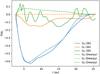 |
Fig. C.1 Internal torques Gx, GY and GZ at time t = 120 yr in units of |
![$\[g_0=\Omega^2 r \Sigma h_p^2\]$](/articles/aa/full_html/2024/09/aa48660-23/aa48660-23-eq20.png)
This is the internal torque vector that we can compare to the internal torque from a 1D warped disk model (e.g., Equation 173 of DKZ22). In Figure C.1 we show these torques in units of ![$\[g_0=\Omega^2 r \Sigma h_p^2\]$](/articles/aa/full_html/2024/09/aa48660-23/aa48660-23-eq21.png) (see Equation 126 of DKZ22). The results show that the GX(r) of the 3D and 1D models match well. This is the torque that is primarily responsible for the wavelike propagation of the warp. The torque GY is the torque that produces a twist. In the 1D model this is perfectly 0, while in the 3D model it is small, but non-zero. The GZ torque component in the 3D model is of the same order of magnitude as GY, and is rather wiggly. Also in the 1D model it is not perfectly zero, which is due to the fact that the disk is not perfectly aligned with the equatorial X − Y plane.
(see Equation 126 of DKZ22). The results show that the GX(r) of the 3D and 1D models match well. This is the torque that is primarily responsible for the wavelike propagation of the warp. The torque GY is the torque that produces a twist. In the 1D model this is perfectly 0, while in the 3D model it is small, but non-zero. The GZ torque component in the 3D model is of the same order of magnitude as GY, and is rather wiggly. Also in the 1D model it is not perfectly zero, which is due to the fact that the disk is not perfectly aligned with the equatorial X − Y plane.
Appendix D Extracting Vr, Vϕ, and Vz from the 3D model
As shown in DKZ22, and following Ogilvie & Latter (2013a), the sloshing motion can be approximated as a linear velocity model
![$\[v_r=V_r \Omega z, \quad v_\phi=V_\phi \Omega z, \quad v_z=V_z \Omega z,\]$](/articles/aa/full_html/2024/09/aa48660-23/aa48660-23-eq22.png) (D.1)
(D.1)
where υz = − υθ by convention. In reality, the functions υr(z), υϕ(z), and υz(z) are only approximately linear in z close to the midplane, but strongly deviate from linearity far away from the midplane, as shown for example in Figure 26. However, usually the strongest deviation occur well above one scale height, while the strongest effect on the disk dynamics is where the density is the highest. A good estimate of V for a velocity υ(z) is:
![$\[V(r, \phi)=\frac{1}{\Sigma H_p^2 \Omega} \int_{-\infty}^{+\infty} \rho(r, \phi, z) v(r, \phi, z) z d z.\]$](/articles/aa/full_html/2024/09/aa48660-23/aa48660-23-eq23.png) (D.2)
(D.2)
The Vr(r, ϕ) is the key component determining the torque. For each r, it can be well approximated by:
![$\[V_r(r, \phi)=V_{r 0}(r) \cos \left(\phi-\phi_{r 0}(r)\right),\]$](/articles/aa/full_html/2024/09/aa48660-23/aa48660-23-eq24.png) (D.3)
(D.3)
where Vr0(r) is the amplitude of the sloshing motion, and ϕr0(r) is the phase shift. As shown in DKZ22, for a Keplerian disk in the wavelike regime, the phase shift, at least in the linear theory, is expected to be ϕr0(r) = 0 if the warp vector is pointing in the ϕ = 0 direction. In that case, the warp evolution is entirely along that same direction, and the disk does not acquire a twist. However, if ϕr0(r) ≠ 0, the disk will acquire a twist, in addition to the wavelike propagation of the warp itself.
From the 3D flattened model we can determine Vr0(r) and ϕr0(r) in the following way: First consider, for each given radius, r,
![$\[V_r(\phi)=A \cos (\phi)+B \sin (\phi).\]$](/articles/aa/full_html/2024/09/aa48660-23/aa48660-23-eq25.png) (D.4)
(D.4)
We now compute A and B as:
![$\[A=\int_{-\pi}^{+\pi} ~V_r(\phi) \cos (\phi) d \phi, \quad B=\int_{-\pi}^{+\pi} V_r(\phi) \sin (\phi) d \phi,\]$](/articles/aa/full_html/2024/09/aa48660-23/aa48660-23-eq26.png) (D.5)
(D.5)
![$\[V_{r 0}(r)=\sqrt{A^2+B^2}, \quad \phi_{r 0}(r)=\tan ^{-1}(B / A).\]$](/articles/aa/full_html/2024/09/aa48660-23/aa48660-23-eq27.png)
References
- Aly, H., Gonzalez, J.-F., Nealon, R., et al. 2021, MNRAS, 508, 2743 [NASA ADS] [CrossRef] [Google Scholar]
- Andrews, S. M. 2020, ARA&A, 58, 483 [Google Scholar]
- Andrews, S. M., Huang, J., Pérez, L. M., et al. 2018, ApJ, 869, L41 [NASA ADS] [CrossRef] [Google Scholar]
- Astropy Collaboration (Price-Whelan, A. M., et al.) 2022, ApJ, 935, 167 [NASA ADS] [CrossRef] [Google Scholar]
- Benisty, M., Juhasz, A., Boccaletti, A., et al. 2015, A&A, 578, A6 [NASA ADS] [CrossRef] [EDP Sciences] [Google Scholar]
- Benisty, M., Stolker, T., Pohl, A., et al. 2017, A&A, 597, A42 [NASA ADS] [CrossRef] [EDP Sciences] [Google Scholar]
- Benisty, M., Juhász, A., Facchini, S., et al. 2018, A&A, 619, A171 [NASA ADS] [CrossRef] [EDP Sciences] [Google Scholar]
- Benítez-Llambay, P., & Masset, F. S. 2016, APJS, 223, 11 [CrossRef] [Google Scholar]
- Bohn, A. J., Benisty, M., Perraut, K., et al. 2022, A&A, 658, A183 [NASA ADS] [CrossRef] [EDP Sciences] [Google Scholar]
- Casassus, S., Marino, S., Pérez, S., et al. 2015, ApJ, 811, 92 [Google Scholar]
- Casassus, S., Avenhaus, H., Pérez, S., et al. 2018, MNRAS, 477, 5104 [NASA ADS] [CrossRef] [Google Scholar]
- Cazzoletti, P., van Dishoeck, E. F., Pinilla, P., et al. 2018, A&A, 619, A161 [NASA ADS] [CrossRef] [EDP Sciences] [Google Scholar]
- Clarke, C. J., & Pringle, J. E. 1993, MNRAS, 261, 190 [Google Scholar]
- Cuello, N., Dipierro, G., Mentiplay, D., et al. 2018, in SF2A-2018: Proceedings of the Annual meeting of the French Society of Astronomy and Astrophysics, eds. P. Di Matteo, F. Billebaud, F. Herpin, N. Lagarde, J. B. Marquette, A. Robin, & O. Venot, Di [Google Scholar]
- Debes, J. H., Poteet, C. A., Jang-Condell, H., et al. 2017, ApJ, 835, 205 [NASA ADS] [CrossRef] [Google Scholar]
- Deng, H., & Ogilvie, G. I. 2022, MNRAS, 512, 6078 [NASA ADS] [CrossRef] [Google Scholar]
- de Val-Borro, M., Edgar, R. G., Artymowicz, P., et al. 2006, MNRAS, 370, 529 [Google Scholar]
- Doğgan, S., Nixon, C. J., King, A. R., Pringle, J. E., & Price, D. 2023, IAU Symp., 362, 177 [Google Scholar]
- Dullemond, C. P., Kimmig, C. N., & Zanazzi, J. J. 2022, MNRAS, 511, 2925 [NASA ADS] [CrossRef] [Google Scholar]
- Facchini, S., Lodato, G., & Price, D. J. 2013, MNRAS, 433, 2142 [Google Scholar]
- Foucart, F., & Lai, D. 2013, ApJ, 764, 106 [NASA ADS] [CrossRef] [Google Scholar]
- Fragner, M. M., & Nelson, R. P. 2010, A&A, 511, A77 [NASA ADS] [CrossRef] [EDP Sciences] [Google Scholar]
- Gammie, C. F., Goodman, J., & Ogilvie, G. I. 2000, MNRAS, 318, 1005 [NASA ADS] [CrossRef] [Google Scholar]
- Garufi, A., Dominik, C., Ginski, C., et al. 2022, A&A, 658, A137 [NASA ADS] [CrossRef] [EDP Sciences] [Google Scholar]
- Gingold, R. A., & Monaghan, J. J. 1977, MNRAS, 181, 375 [NASA ADS] [CrossRef] [Google Scholar]
- Harris, C. R., Millman, K. J., van der Walt, S. J., et al. 2020, Nature, 585, 357–362 [NASA ADS] [CrossRef] [Google Scholar]
- Hopkins, P. F. 2015, MNRAS, 450, 53 [Google Scholar]
- Hunter, J. D. 2007, Comput. Sci. Eng., 9, 90 [NASA ADS] [CrossRef] [Google Scholar]
- Icke, V. 1991, A&A, 251, 369 [NASA ADS] [Google Scholar]
- Kraus, S., Kreplin, A., Young, A. K., et al. 2020, Science, 369, 1233 [NASA ADS] [CrossRef] [Google Scholar]
- Kuffmeier, M., Dullemond, C. P., Reissl, S., & Goicovic, F. G. 2021, A&A, 656, A161 [NASA ADS] [CrossRef] [EDP Sciences] [Google Scholar]
- Lodato, G., & Facchini, S. 2013, MNRAS, 433, 2157 [NASA ADS] [CrossRef] [Google Scholar]
- Lodato, G., & Price, D. J. 2010, MNRAS, 405, 1212 [NASA ADS] [Google Scholar]
- Lubow, S. H., & Ogilvie, G. I. 2000, ApJ, 538, 326 [CrossRef] [Google Scholar]
- Manara, C. F., Ansdell, M., Rosotti, G. P., et al. 2023, in ASP Conf. Ser., 534, Protostars and Planets VII, eds. S. Inutsuka, Y. Aikawa, T. Muto, K. Tomida, & M. Tamura, 539 [Google Scholar]
- Marino, S., Perez, S., & Casassus, S. 2015, ApJ, 798, L44 [Google Scholar]
- Martin, R. G., Lubow, S. H., Pringle, J. E., et al. 2019, ApJ, 875, 5 [NASA ADS] [CrossRef] [Google Scholar]
- Min, M., Stolker, T., Dominik, C., & Benisty, M. 2017, A&A, 604, L10 [NASA ADS] [CrossRef] [EDP Sciences] [Google Scholar]
- Monaghan, J. J. 2005, Rep. Progr. Phys., 68, 1703 [Google Scholar]
- Muro-Arena, G. A., Benisty, M., Ginski, C., et al. 2020, A&A, 635, A121 [NASA ADS] [CrossRef] [EDP Sciences] [Google Scholar]
- Nagasawa, M., Ida, S., & Bessho, T. 2008, ApJ, 678, 498 [NASA ADS] [CrossRef] [Google Scholar]
- Nealon, R. 2018, in Take a Closer Look, 38 [Google Scholar]
- Nelson, R. P., & Papaloizou, J. C. B. 1999, MNRAS, 309, 929 [CrossRef] [Google Scholar]
- Nealon, R., Pinte, C., Alexander, R., Mentiplay, D., & Dipierro, G. 2019, MNRAS, 484, 4951 [CrossRef] [Google Scholar]
- Nealon, R., Cuello, N., & Alexander, R. 2020a, MNRAS, 491, 4108 [NASA ADS] [Google Scholar]
- Nealon, R., Price, D. J., & Pinte, C. 2020b, MNRAS, 493, L143 [NASA ADS] [CrossRef] [Google Scholar]
- Nixon, C., & King, A. 2016, in Lect. Notes Phys., 905, eds. F. Haardt, V. Gorini, U. Moschella, A. Treves, & M. Colpi (Berlin Springer Verlag), 45 [NASA ADS] [CrossRef] [Google Scholar]
- Ogilvie, G. I. 1999, MNRAS, 304, 557 [NASA ADS] [CrossRef] [Google Scholar]
- Ogilvie, G. I., & Latter, H. N. 2013a, MNRAS, 433, 2420 [NASA ADS] [CrossRef] [Google Scholar]
- Ogilvie, G. I., & Latter, H. N. 2013b, MNRAS, 433, 2403 [NASA ADS] [CrossRef] [Google Scholar]
- Papaloizou, J. C. B., & Lin, D. N. C. 1995, ApJ, 438, 841 [NASA ADS] [CrossRef] [Google Scholar]
- Papaloizou, J. C. B., & Pringle, J. E. 1983, MNRAS, 202, 1181 [NASA ADS] [Google Scholar]
- Papaloizou, J. C. B., & Terquem, C. 1995, MNRAS, 274, 987 [NASA ADS] [Google Scholar]
- Papaloizou, J. C. B., Korycansky, D. G., & Terquem, C. 1995, Ann. N. Y. Acad. Sci., 773, 261 [NASA ADS] [CrossRef] [Google Scholar]
- Papaloizou, J. C. B., Larwood, J. D., Nelson, R. P., & Terquem, C. 1997, in Accretion Disks – New Aspects, 487, eds. E. Meyer-Hofmeister & H. Spruit, 182 [CrossRef] [Google Scholar]
- Pérez, L. M., Benisty, M., Andrews, S. M., et al. 2018, ApJ, 869, L50 [CrossRef] [Google Scholar]
- Pinte, C., Dent, W. R. F., Ménard, F., et al. 2016, ApJ, 816, 25 [Google Scholar]
- Poon, M., Zanazzi, J. J., & Zhu, W. 2021, MNRAS, 503, 1599 [CrossRef] [Google Scholar]
- Pringle, J. E. 1992, MNRAS, 258, 811 [NASA ADS] [CrossRef] [Google Scholar]
- Rabago, I., Zhu, Z., Martin, R. G., & Lubow, S. H. 2023, MNRAS, 520, 2138 [NASA ADS] [CrossRef] [Google Scholar]
- Rabago, I., Zhu, Z., Lubow, S., & Martin, R. G. 2024, MNRAS, 533, 360 [NASA ADS] [CrossRef] [Google Scholar]
- Sai, J., Ohashi, N., Saigo, K., et al. 2020, ApJ, 893, 51 [NASA ADS] [CrossRef] [Google Scholar]
- Shakura, N. I., & Sunyaev, R. A. 1973, A&A, 24, 337 [NASA ADS] [Google Scholar]
- Smallwood, J. L., Nealon, R., Chen, C., et al. 2021, MNRAS, 508, 392 [NASA ADS] [CrossRef] [Google Scholar]
- Sorathia, K. A., Krolik, J. H., & Hawley, J. F. 2013, ApJ, 768, 133 [NASA ADS] [CrossRef] [Google Scholar]
- Stolker, T., Sitko, M., Lazareff, B., et al. 2017, ApJ, 849, 143 [Google Scholar]
- Van Rossum, G., & Drake, F. L. 2009, Python 3 Reference Manual (Scotts Valley, CA: CreateSpace) [Google Scholar]
- Villenave, M., Ménard, F., Dent, W. R. F., et al. 2020, A&A, 642, A164 [EDP Sciences] [Google Scholar]
- Virtanen, P., Gommers, R., Oliphant, T. E., et al. 2020, Nature Methods, 17, 261 [CrossRef] [Google Scholar]
- Zanazzi, J. J., & Lai, D. 2018a, MNRAS, 477, 5207 [NASA ADS] [CrossRef] [Google Scholar]
- Zanazzi, J. J., & Lai, D. 2018b, MNRAS, 473, 603 [NASA ADS] [CrossRef] [Google Scholar]
All Tables
All Figures
|
Fig. 1 Schematics of the spherical grid set-up in our simulations. The poles are cut off in order to save computation time. |
| In the text | |
|
Fig. 2 Aspect ratio (i.e., pressure scaleheight scaled with radius) h(r) = Hp(r)/r of our initial set-up. The black dashed line is the analytical calculation according to Eq. (5), the pink solid line shows the Gaussian fit from the initial set-up in our simulation. Gray dotted and dashed lines indicate the reference radius R0 = 5.2 au and the corresponding reference aspect ratio h0 = 0.05, respectively. |
| In the text | |
|
Fig. 3 Surface density (top panel) and inclination (bottom panel) evolution of a disk aligned to the grid midplane. The color in the bottom panel highlights the time. The simulation covers a time span of 6000 yr, which are 500 orbits at the reference radius, R0 = 5.2 au. |
| In the text | |
|
Fig. 4 Cross-section through the initial tilted disk along the x-axis. |
| In the text | |
|
Fig. 5 Similar to Fig. 3, but for the a disk tilted by 10° with respect to the grid midplane. The additional panel at the bottom shows the precession angle of the disk. The grey dashed lines indicate the inclination oscillation periods investigated in Fig. 7. |
| In the text | |
|
Fig. 6 Surface density evolution of a tilted disk by 10° in simulations with different boundary conditions. The top panel shows our fiducial set-up with rigid boundaries, the middle is the same set-up, but with the outflow boundary conditions at the inner edge, and the bottom panel has an exponential cutoff at outer and inner edge, in addition to inner outflow boundary conditions. |
| In the text | |
|
Fig. 7 Inclination profile evolution during the first and second periods of the inclination oscillation. Each period is indicated by the color scale from blue to yellow. The first period extends from 420 to 1140 yr, the second from 1140 to 1860 yr. |
| In the text | |
|
Fig. 8 Inclination (top panel) and precession angle (bottom panel) in simulations with varying resolutions in a disk tilted by 10° with respect to the grid midplane. |
| In the text | |
|
Fig. 9 Same as Fig. 8, but for simulations using varying viscosities. The disks are still tilted by 10° with respect to the grid midplane. The dotted lines show the same simulations with higher resolution in θ-direction (corresponding to theta_resolution in Table 1). |
| In the text | |
|
Fig. 10 Inclination (top panel) and precession (bottom panel) evolution of a disk tilted by 30° with respect to the grid midplane. |
| In the text | |
|
Fig. 11 Cross-section of the initial warped disk along the x-axis. |
| In the text | |
|
Fig. 12 Evolution of the inclination profile in the warped disk simulation. The color simply highlights the time. |
| In the text | |
|
Fig. 13 Long-term evolution of the inclination profile in the warped disk simulation. |
| In the text | |
|
Fig. 14 Decay of inclination in the warped disk simulation. We chose to evaluate the inclination close to the outer edge at a radius of 22.5 au. The black line shows the simulation data, the blue dashed line the fit. The grey dashed line indicates the starting point of the fit. |
| In the text | |
|
Fig. 15 Inclination evolution of the warped disk in comparison between the 3D set-up in FARGO3D (left panel) and the 1D set-up in dwarpy (right panel). For comparability, we plot until 240 yr of simulated time. Note that the computational domain of the 1D simulation is well beyond the outer edge of the figure. |
| In the text | |
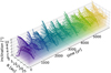 |
Fig. 16 Same as Fig. 12, but for the 1D model with dwarpy. |
| In the text | |
|
Fig. 17 Direction of the total angular momentum vector in the beginning of the simulation t = 0 yr (grey dashed line) and in the end t = 2.4 × 10⁴ yr (solid black line). The line connecting the two arrows indicates the time evolution with darker color the later the time. |
| In the text | |
|
Fig. 18 Twist motion in the warped disk simulation. Top row: unit angular momentum vectors close to the inner (left panel) and outer (right panel) edge of the disk for the first t = 6000 yr. Similar to Fig. 17. Middle row: x-y components of the unit angular momentum vector at the same radii as in the top row, but only for the time period between 300 and 390 orbits at R0, chosen to roughly show 1.5 precession periods. The direction of the precession is indicated by the arrows. x-markers show the beginning of the plotted time, squares the end. Diamonds indicate the middle of this time period (45 orbits after the x-markers). Bottom row: same as middle row, but for various radii, plotted with an offset of r/(60 au) in y-direction to disentangle the twist at different radii. The stars show the lx−ly components at a snapshot at t = 3696 yr (308 orbits at R0), which shows a twisted state in the time evolution. |
| In the text | |
|
Fig. 19 Cross-section along the x-axis of the locally isothermal warped disk. |
| In the text | |
 |
Fig. 20 Evolution of the inclination profile in the locally isothermal warped disk. Like Fig. 20. |
| In the text | |
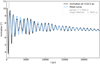 |
Fig. 21 Like Fig. 14, but for the locally isothermal disk. |
| In the text | |
|
Fig. 22 Inclination evolution at radius r = 22.5 au (black solid lines) in simulations with different disk viscosities. The blue dashed lines indicate the fit according to Eq. (11). The middle panel corresponds to the fiducial simulation and is the same as Fig. 14. |
| In the text | |
|
Fig. 23 Precession angles for different radii (colored lines) in simulations with different disk viscosities. The black dashed line in each panel shows the precession angle of the angular momentum vector, Ltot, of the whole disk. The grey dotted lines indicate precession periods of roughly 740 yr. |
| In the text | |
|
Fig. 24 Gas density of the disk annulus at r = 8.3 au at time t = 120 yr. The map is a standard (ϕ, θ) projection of the sphere of constant distance to the star. The color scale is linear. Left: in unrotated coordinates. Right: in rotated coordinates such that the disk annulus lies in the equatorial plane. |
| In the text | |
|
Fig. 25 Gas velocity components in units of the local isothermal sound speed at r = 8.3 au at time t = 120 yr, in the rotated frame (as in Fig. 24-right). The colors are linear between −1 and 1, and logarithmic for |υ/cs| > 1. Note: the isothermal sound speed cs is constant at 0.66 kms−1 throughout each panel, consistent with a disk aspect ratio of hp/r = 0.064. Left: Radial velocity (sloshing motion). Right: Vertical velocity (breathing motion). The dot-dashed, dashed and dotted grey lines mark the rms vertical extend of the disk (which would relate to the pressure scale height in a steady-state disk), twice that, and three times that. The grey areas below and above are the regions outside the model grid. |
| In the text | |
|
Fig. 26 Radial gas velocity in units of the local isothermal sound speed, at the same radius and time as in Fig. 25, at azimuth ϕ = 1.29, i.e., a vertical slice of that figure. The blue curve shows the data from the 3D model, the orange curve a linear reconstruction using a slope computed as in Appendix D. |
| In the text | |
|
Fig. A.1 Evolution of the inclination profile in the high-resolution warped disk simulation. The color highlights the time. Similar to Figure 12. |
| In the text | |
|
Fig. A.2 Decay of inclination in the high resolution warped disk simulation. We evaluate the inclination at r = 22.5 au. The black line shows the simulation data, the blue dashed line shows the fit. The grey dashed line indicates the starting point of the fit. Similar to Figure 14 (note the slightly shorter simulation time). |
| In the text | |
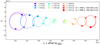 |
Fig. A.3 Twist of the disk in the high resolution simulation (like Figure 18, bottom panel). |
| In the text | |
|
Fig. A.4 Precession angles for different radii (colored lines) in simulations with different resolutions. The black dashed line in each panel shows the precession angle of the angular momentum vector Ltot of the whole disk. The grey dotted lines indicate precession periods of roughly 740 yr. Similar to Figure 23. |
| In the text | |
|
Fig. B.1 Set-up of a warped disk with the outer boundary further away from the physical disk edge. |
| In the text | |
|
Fig. B.2 Twist of a disk with the outer boundary far away from the disk edge, like Figure 18, bottom panel. |
| In the text | |
|
Fig. B.3 Surface density of a disk with the outer boundary far away from the disk edge (solid lines). The initial state of the fiducial simulation is plotted as reference (dashed line). |
| In the text | |
|
Fig. B.4 Evolution of the twisted state in a 1D simulation using dwarpy in two different simulations. The initial state of the warp in both simulations is taken from the twisted state in the 3D simulation at t = 3696 yr (308 orbits at R0). The top panel shows the 1D simulation with internal torque G extracted from the 3D simulation, the bottom panel shows the same simulation, but internal torque G initially set to zero for comparison. Details comparable to Figure 18 (bottom panel). |
| In the text | |
|
Fig. B.5 Azimuthal velocity (top panel) and the residuals from the Kepler velocity (bottom panel). The black dashed line shows the Kepler velocity. |
| In the text | |
|
Fig. B.6 Twist motion in the locally isothermal disk. Top: Unit angular momentum vectors close to the inner (left panel) and outer (right panel) edge of the disk for the first t = 6000 yr. Bottom: x-y-components of the unit angular momentum vector for the time period between 300–390 orbits at R0 at varying radii, plotted with an offset of r/(60 au) in y-direction to disentangle the twist at different radii. The x-markers show the beginning of the plotted time, the squares the end. Similar to Figure 18. |
| In the text | |
|
Fig. C.1 Internal torques Gx, GY and GZ at time t = 120 yr in units of |
| In the text | |
Current usage metrics show cumulative count of Article Views (full-text article views including HTML views, PDF and ePub downloads, according to the available data) and Abstracts Views on Vision4Press platform.
Data correspond to usage on the plateform after 2015. The current usage metrics is available 48-96 hours after online publication and is updated daily on week days.
Initial download of the metrics may take a while.