© The Authors 2024

1. Introduction

GSN 069 is the first galaxy found to have X-ray quasi-periodic eruptions (QPEs), which originate in the region around the supermassive black hole (SMBH) (Miniutti et al. 2019). The nature of the QPEs is still unclear, and its period ∼9 h may correspond to the orbital period of a body orbiting the SMBH, but the radiative processes and the nature of the body are controversial (King 2020, 2022; Chen et al. 2022; Zhao et al. 2022; Wang et al. 2022; Krolik & Linial 2022; Lu & Quataert 2023; Xian et al. 2021; Suková et al. 2021; Linial & Sari 2023; Linial & Metzger 2023).

Although QPEs have since been seen in other galaxies (Giustini et al. 2020; Song et al. 2020a; Arcodia et al. 2021; Chakraborty et al. 2021), GSN 069 remains the most exceptional one. It is the only galaxy with QPEs associated with a TDE, which has a 500 − 800 day timescale and is found to be re-brightening after 9 years since the main peak appeared (Shu et al. 2018; Miniutti et al. 2023). The abnormal carbon and nitrogen abundance ratio in its spectrum suggests that it is likely the disruption of a red giant (Sheng et al. 2021), whose core will continue to exist as a white dwarf (WD). This is consistent with the suggestion by King (2020) that the QPEs of GSN 096 come from a tidally stripped WD by the SMBH.

The origin of this TDE is puzzling. The orbital period of the disrupted star must be longer than the timescale of the TDE, which is much longer than the period of the QPEs. So if we assume that the disrupted star is the progenitor of the orbiting current star, then this star needs to have undergone a drastic change in orbital period after being partially disrupted. This change can be explained by the Hills mechanism, where the current orbiting star is captured by the SMBH from a binary system (Hills 1988; Wang et al. 2022). Although the orbital period of the binary system and the SMBH can be very long at this time, the orbital velocity of the disrupted star with respect to the centre of mass of the binary also affects the timescale of the TDE.

In this Letter, we show that the disruption of the envelope of a single star always predicts a much shorter timescale than the observational value, which is shown in Sect. 2. So we suggest the TDE from GSN 069 is the disruption of a common envelope (CE), and we explain how we calculated its fallback rate in Sect. 3. We provide information on how we applied this model on GSN 069 in Sect. 4 and discussions in Sect. 5.

2. TDE of the envelope of a single star

The fallback timescale of TDE is determined by the specific binding energy of the most bound material

$$\begin{array}{c}\hfill t_{\mathrm{fb}}=2\pi G{M}_{\mathrm{BH}}{(-2ϵ)}^{-3/2},\end{array}$$(1)

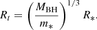
where the G is the gravitational constant, M_BH is the mass of the SMBH, and ϵ is the specific binding energy.

If the orbit of the disrupted star is eccentric, the specific binding energy of the disrupted star ϵ_i is not equal to zero, and therefore it needs to be considered. The specific binding of the most bound debris is

$$\begin{array}{c}\hfill ϵ\approx {ϵ}_i+\frac{G{M}_{\mathrm{BH}}}{R_t^2}{R}_{\ast }.\end{array}$$(2)

Here the second term is the specific binding energy for the parabolic orbit (Gezari 2021), R_t is the disruption radius, and R_* is the radius of the disrupted star.

We assume that the averaged period of 9 h for QPEs in GSN 069 corresponds to the orbital period of a WD orbiting an SMBH. If the TDE from GSN 069 is the disruption of an evolved star after it is captured, ϵ_i is equal to its specific binding energy. Then the fallback timescale of the TDE is smaller than the orbital period of the evolved star, which is also equal to the orbital period of the orbiting remnant WD. It is much smaller than the observed timescale of the TDE in GSN 069, which is about 500 − 800 days (Miniutti et al. 2023). In this case, the first term in Eq. (2) is dominant, so a situation needs to be found to make it high enough to achieve the observed timescale.

So the disruption must occur before the capture of the WD. In this case, the velocity of the disrupted envelope contains two components: the orbital velocity of the disrupted star v_* and the velocity of the binary v_b relative to the SMBH. Assuming the binary is in a parabolic orbit, the specific binding energy of the disrupted star is

$$\begin{array}{c}\hfill {ϵ}_i\approx v_{\ast }{v}_{b}cos\theta ,\end{array}$$(3)

where θ is the angle between v_* and v_b. The $v_{*}^2/2$ term is ignored.

Assuming the WD is captured at the periastron by the Hills mechanism, the capture of the WD corresponds to θ = π, so the timescale corresponding to the specific binding energy ϵ_i ≈ −v_*v_b is the orbital period of captured WD. If θ is close to 0 while the disruption occurs, corresponding to the situation that the disrupted star is the companion of the captured WD, the disrupted envelope is subsequently fully unbound. In this case, Eq. (2) leads to a positive binding energy because ϵ_i = v_*v_b is much higher than the second term. So to produce the observational long timescale, ϵ_i needs to be close to zero, which means θ needs to be close to π/2 at the moment of disruption.

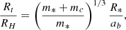
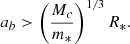
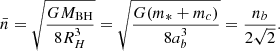
So the disruption distance needs to be sufficiently larger than the capture distance to ensure the angle θ is close to π/2. The capture distance is (Amaro-Seoane 2018)

$$\begin{array}{c}\hfill R_H={\left(\frac{M_{\mathrm{BH}}}{m_b}\right)}^{1/3}{a}_b.\end{array}$$(4)

Here m_* and m_c are the mass of the disrupted star and its companion, respectively. We note that m_b = m_* + m_c is the total mass of the binary, and a_b is the separation of the binary.

The disruption radius is (Gezari 2021)

$$\begin{array}{c}\hfill R_t={\left(\frac{M_{\mathrm{BH}}}{m_{\ast }}\right)}^{1/3}{R}_{\ast }.\end{array}$$(5)

So the ratio of these two radii is

$$\begin{array}{c}\hfill \frac{R_t}{R_H}={\left(\frac{m_{\ast }+m_c}{m_{\ast }}\right)}^{1/3}\frac{R_{\ast }}{a_b},\end{array}$$(6)

which is independent of the mass of the SMBH. To avoid the disruption of the evolved star by the companion, the separation needs to satisfy

$$\begin{array}{c}\hfill a_b>{\left(\frac{M_c}{m_{\ast }}\right)}^{1/3}{R}_{\ast }.\end{array}$$(7)

And the companion is outside the envelope of the evolved star, requiring

$$\begin{array}{c}\hfill a_b>R_{\ast }+R_c.\end{array}$$(8)

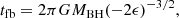
The above two conditions together give the upper limit of R_t/R_H. As shown in Fig. 1, R_t can be larger than R_H when the companion is much more compact than the disrupted star, and the maximum R_t is about 1.25R_H.

Fig. 1. Value of the upper limit of Rt/RH for the companion star of various densities and masses. Here ρc and ρ* are the average density of the companion and the disrupted star, respectively. The solid line represents Rt/RH = 1.

The time for the binary to move from distance R_t to periastron R_H is

$$\begin{array}{c}\hfill t=-\frac{\frac{1}{2}tan\frac{f}{2}+\frac{1}{6}{tan}^3\frac{f}{2}}{\overline{n}},\end{array}$$(9)

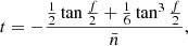
where f is the true anomaly, and it can be obtained by ${sec}^2\frac{f}{2}=R_t/R_H$ (f is negative). Furthermore, $\overline{n}$ is the averaged angular velocity

$$\begin{array}{c}\hfill \overline{n}=\sqrt{\frac{G{M}_{\mathrm{BH}}}{8R_H^3}}=\sqrt{\frac{G(m_{\ast }+m_c)}{8a_b^3}}=\frac{n_b}{2\sqrt{2}}.\end{array}$$(10)

Here $n_b=\sqrt{G(m_{\ast }+m_c)/a_b^3}$ is the angular velocity of the binary. So the change in the direction of the orbital position caused by orbital motion in the binary is

$$\begin{array}{c}\hfill \mathrm{\Delta }\eta =-n_{b}t=\sqrt{2}tan\frac{f}{2}+\frac{\sqrt{2}}{3}{tan}^3\frac{f}{2}.\end{array}$$(11)

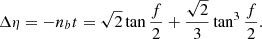
Figure 1 gives an upper limit of R_t/R_H of about 1.25, which corresponds to a minimum f. So the maximum Δη_max can be obtained by Eq. (11) and it is about 0.766 rad. Due to the maximum of R_t/R_H being small, the change in the direction of the orbital velocity of the binary in the parabolic orbit can be ignored. So the change of θ in Eq. (3) is roughly equal to Δη. Due to θ = π at the capture distance, the θ at the disruption distance is π − Δθ.

So Δθ_max corresponds to a maximum ϵ_i ≈ −0.72v_*v_b. Combined with t_fb ∼ ( − ϵ)^−3/2, the maximum timescale of TDE in this situation is about 1.6 times the orbital period of the captured WD ∼ 14.4 h, which is still much smaller than the observational value.

Now, we can safely rule out the situations in which TDE from GSN 069 is the disruption of the envelope of either of the stars in the binary. The one remaining possible scenario is that it is the disruption of a CE that contains the double stars in it. In this scenario, the velocity of the envelope is the orbital velocity, and ϵ_i is zero for a parabolic orbit. So the observational timescale of the TDE can be produced easily.

3. TDE of the CE

The structure of the CE is still unclear (Ivanova et al. 2013). Here we only consider the effect of the differential rotation of the CE. We adopted a similar model as early works¹ (Meyer & Meyer-Hofmeister 1979; Meng & Podsiadlowski 2017; Song et al. 2020b). The envelope is co-rotating with the binary at the centre and the rotational velocity decreases outwards, following a radial power law. The rotational angular velocity can be described by

$$\begin{array}{c}\hfill \mathrm{\Omega }=\{\begin{array}{cc}{\mathrm{\Omega }}_0,\hfill & s\le s_0\hfill \\ {\mathrm{\Omega }}_0{\left(\frac{s}{s_0}\right)}^{-\alpha },\hfill & s>s_0\hfill \end{array},\end{array}$$(12)

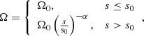
where s is the distance to the rotational axis, and s₀ and Ω₀ are the distance and the rotational angular velocity at the boundary of the binary, respectively.

3.1. Effect of rotation on specific binding energy

Under the frozen-in approximation, the fallback rate of the TDE is (Gezari 2021)

$$\begin{array}{c}\hfill \dot{M}=\frac{\mathrm{d}M}{\mathrm{d}ϵ}\frac{\mathrm{d}ϵ}{\mathrm{d}t}=\frac{2\pi }{3}{\left(G{M}_{\mathrm{BH}}\right)}^{2/3}\frac{\mathrm{d}M}{\mathrm{d}ϵ}{t}^{-5/3}.\end{array}$$(13)

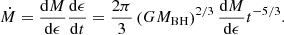
It strongly depends on the distribution of the specific binding energy in the star.

The rotation can affect the specific binding energy by providing an additional speed. Assuming the centre of mass (COM) is on a parabolic orbit, the specific binding energy with rotation is (Golightly et al. 2019)

$$\begin{array}{c}\hfill ϵ\approx (\mathit{v}\times \mathbf{\Omega }+\frac{G{M}_{\mathrm{BH}}}{R_t^3}{\mathit{R}}_t)·\mathit{r}.\end{array}$$(14)

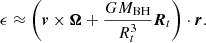
Here v and R_t are the velocity and the position of the COM relative to the central black hole while the star begins to be disrupted, respectively. Furthermore, Ω is the rotational angular velocity, and r is the position within the star relative to the COM. Only the lowest order of the rotation has been considered for this Letter.

The specific binding energy can also be viewed as a projection of the position r in the direction 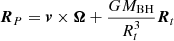${\mathit{R}}_P=\mathit{v}\times \mathbf{\Omega }+\frac{G{M}_{\mathrm{BH}}}{R_t^3}{\mathit{R}}_t$, and it only depends on the projection distance. For the case of the rigid rotation, the projection vector R_P is independent of the position r, as in the case of no rotation (Ω = 0). Thus, the star with rigid rotation has a similar distribution to the specific binding energy with the star without rotation. Both of them have isoenergetic surfaces that are the plane perpendicular to the projection vector R_P, and only the magnitude of the specific binding energy is different. So the disruption of the star with rigid rotation has a similar evolution to the fallback rate with the star without rotation, as shown in Golightly et al. (2019).

If the rotation is differential, the projection vector R_P is dependent on the position r. Then the equipotential surfaces are no longer planar but curved, which depends on the distribution of the rotation Ω.

Here we consider a simple case. A CE with mass M_* and radius R_* is disrupted at the periastron, and vector Ω is perpendicular to the orbital plane, which means that the $\widehat{v}$, $\widehat{\mathrm{\Omega }}$, and ${\widehat{R}}_t$ are perpendicular to each other. With $\widehat{\mathrm{\Omega }}$ as the z-axis and ${\widehat{R}}_t$ as the x-axis, using the cylindrical coordinate (s, ϕ, z), Eq. (14) can be rewritten as

$$\begin{array}{cc}& ϵ=s(\frac{G{M}_{\mathrm{BH}}}{R_t^2}+\mathrm{\Omega }v)cos\varphi \hfill \\ \hfill & ={ϵ}_0\overline{s}(1+k{\overline{s}}^{-\alpha })cos\varphi .\hfill \end{array}$$(15)

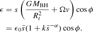
Here $\overline{s}\equiv s/R_{\ast }$ is the normalized distance. Furthermore, ${ϵ}_0\equiv G{M}_{\text{BH}}{R}_{*}/R_t^2$ is the standard specific binding energy of the envelope without rotation. We assume that the angular velocity is the power law, for example $\mathrm{\Omega }={\mathrm{\Omega }}_{\mathrm{s}}{\overline{s}}^{-\alpha }$, where Ω_s is the rotational velocity on the surface of the envelope. The parameter k is

$$\begin{array}{cc}& k\equiv \frac{{\mathrm{\Omega }}_{\mathrm{s}}v}{(G{M}_{\mathrm{BH}}/R_t^2)}={\mathrm{\Omega }}_{\mathrm{s}}\sqrt{\frac{2R_t^3}{G{M}_{\mathrm{BH}}}}\hfill \\ \hfill & =\sqrt{2}\frac{{\mathrm{\Omega }}_{\mathrm{s}}}{{\mathrm{\Omega }}_{\ast }}=k_0{\overline{s}}_0^{\alpha -\frac{3}{2}},\hfill \end{array}$$(16)

where $k_0\equiv \sqrt{2M_c/M_{\ast }}$. In the derivation of the above equation, the velocity of the parabolic orbit $v=\sqrt{2G{M}_{\mathrm{BH}}/R_t}$, and the disrupted radius R_t = (M_BH/M_*)^1/3R_* is adopted. In addition, ${\mathrm{\Omega }}_{\ast }\equiv \sqrt{G{M}_{\ast }/R_{\ast }^3}$ is the break-up rotation velocity of the star.

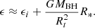
We show an example of the $\overline{ϵ}=ϵ/{ϵ}_0$ distribution with k₀ = 1, $\overline{s}=0.1$, and α = 3 in Fig. 2, and the regions of interest are with $\overline{ϵ}<0$. There is a stationary point near which the change in $\overline{ϵ}$ slows down. The isoenergetic surface through this point delineates the distribution of $\overline{ϵ}$ into four regions. As shown in Fig. 2, the region with the lowest $\overline{ϵ}$ is to the right of the stationary point, the left side region has a higher $\overline{ϵ}$, and the highest $\overline{ϵ}$ is distributed in both the upper and lower regions. A smaller gradient of $\overline{ϵ}$ near the stationary point predicts a higher dM/dϵ here and therefore a peak in the fallback rate.

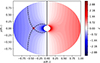Fig. 2. Distribution of $\overline{ϵ}$ with k0 = 1, ${\overline{s}}_0=0.1$, and α = 3. The red star is the stationary point, and the corresponding $\overline{ϵ}$ is represented by the dashed line. The solid line represents $\overline{ϵ}=0$, and $\overline{ϵ}$ is negative on its left side and positive on its right side.

Because the SMBH is in the direction of ϕ = π, the position of the stationary point can be obtained by solving for the minimum value of Eq. (15) with cos ϕ = −1,

$$\begin{array}{c}\hfill {\overline{s}}_{\mathrm{p}2}={(k(\alpha -1))}^{1/\alpha },\end{array}$$(17)

which corresponds to the specific binding energy

$$\begin{array}{c}\hfill {\overline{ϵ}}_{\mathrm{p}2}=-\frac{\alpha {(k(\alpha -1))}^{1/\alpha }}{\alpha -1}.\end{array}$$(18)

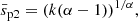
The subscript p2 indicates that it is the second peak. Then the time of the second peak can be obtained by Eq. (1).

The apparent time of the second peak depends on the distribution of the angular velocity in the envelope. For a given α, the higher k is, the smaller $\overline{ϵ}$, which predicts the earlier second peak.

3.2. Fallback rate

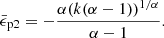
The mass of disrupted star can be expressed as $M=\iiint \rho \overline{s}\mathrm{d}\overline{s}\mathrm{d}\overline{z}\mathrm{d}\varphi$. By transformation from cylindrical coordinate $(\overline{s},\varphi ,\overline{z})$ to coordinate $(\overline{s},\overline{ϵ},\overline{z})$, it becomes

$$\begin{array}{cc}& \frac{\mathrm{d}M}{\mathrm{d}ϵ}=\frac{-2}{{ϵ}_0}{\displaystyle \int \int }\left|\frac{\partial (\overline{s},\varphi ,\overline{z})}{\partial (\overline{s},\overline{ϵ},\overline{z})}\right|\rho \overline{s}\mathrm{d}\overline{s}\mathrm{d}\overline{z}\hfill \\ \hfill & =\frac{2}{{ϵ}_0}{\displaystyle \int }\frac{{\rho }_z\overline{s}}{\sqrt{{\overline{s}}^2{(1+k{\overline{s}}^{-\alpha })}^2-{\overline{ϵ}}^2}}\mathrm{d}\overline{s}.\hfill \end{array}$$(19)

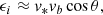
Here ρ_z ≡ ∫ρdz is the column density. Then the fallback rate can be obtained by Eq. (13). Here we show the fallback rate with R_* = 1 R_⊙, M_* = 1 M_⊙, M_BH = 10⁶ M_⊙, α = 3, and k₀ = 1 in Fig. 3. The disrupted star is assumed to be spherical, and the density is assumed to be constant.

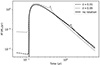Fig. 3. Fallback rate for the different rotation. Comparing the case of no rotation, the disruption of the envelope with differential rotation shows a second peak in the decay phase. The larger the core, the earlier the peak appears. The earlier fallback with differential rotation is caused by the innermost material, which has the lowest specific binding energy.

Comparing the curve of the envelope without rotation, the disruption of the envelope with differential rotation as expected shows a second peak. A larger core leads to the stationary point further away from the core, thus producing earlier peaks that are also stronger. Before this peak appears, the curve decays similarly to the case without rotation, due to the small rotation of the material in the outer layers of the disrupted envelope. The fallback before the main peak is the accretion of the innermost material, which has the smallest binding energy.

4. Application to the TDE in GSN 069

Although our calculated fallback rate reproduces the second peak of the observational light curve, a direct comparison between the full light curve and our model is inappropriate. Under the frozen-in approximation, pressure and self-gravity in the accretion flow are neglected. In Fig. 3 it can be seen that the material near the core has the smallest fallback timescale, and it may interact with material near the stationary point thereby exchanging energy while moving outwards, which leads to the broadening of the second peak. Furthermore, since the stationary point corresponds to a region of high density in the accretion flow, self-gravity could potentially lead to self-bound material around the stationary point and thus narrow the second peak. However, these effects only affect the shape of the second peak and not the time of its appearance.

The gravitation of the core significantly affects the fallback curve and can make it go from a −5/3 decay to a −9/4 decay, which is the curve of a partial tidal disruption event (Coughlin & Nixon 2019). Considering that material closer to the core is affected by a stronger gravitation of the core relative to the gravitation of the SMBH, the fallback timescales of material near the stationary point are expected to be modified more than those of the most bounded material. Thus, the ratio of the time of appearance of the second peak to the main peak should become larger. On the other hand, the captured star may also affect the motion of the disrupted envelope. These effects cannot be solved analytically, so we ignore them for now in the discussion that follows.

The density distribution of the disrupted envelope also significantly affects the fallback curve. The realistic density distribution of the CE should be quite different from the constant density we assumed. Although its exact distribution is not known, the stationary point that appears in the specific binding energy distribution still produces a peak in the fallback rate curve as long as the density distribution is relatively smooth.

Therefore, the only parameter that can be used to make comparisons with observations is the relative time between the appearance of the second peak and the main peak. The specific binding energy of the most bound material is ${\overline{ϵ}}_{\mathrm{p}1}=-(1+k)$ by Eq. (15), where the subscript p1 represents the main peak. The ratio of the fallback time between the main peak and the second peak is

$$\begin{array}{c}\hfill \frac{t_{\mathrm{p}2}}{t_{\mathrm{p}1}}={\left(\frac{{\overline{ϵ}}_{\mathrm{p}2}}{{\overline{ϵ}}_{\mathrm{p}1}}\right)}^{-3/2}={\left(\frac{\alpha {(k(\alpha -1))}^{1/\alpha }}{(\alpha -1)(1+k)}\right)}^{-3/2},\end{array}$$(20)

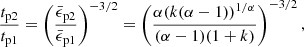
which only depends on the rotation distribution of the CE.

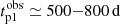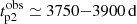Miniutti et al. (2023) fitted the light curve of the two peaks of the TDE from GSN 069 using a formula of Gaussian rise plus power-law decay with the index −9/4. They found $t_{\mathrm{p}1}^{\mathrm{obs}}\simeq 500-800\mathrm{d}$ and $t_{\mathrm{p}2}^{\mathrm{obs}}\simeq 3750-3900\mathrm{d}$. We adopted their median value and obtained (t_p2/t_p1)_obs ≃ 4.7 − 7.8.

They found the accreted mass is about M_accr = 0.23 M_⊙ by integrating the light curve as well. So the mass of the disrupted envelope is about 0.46 M_⊙ considering the unbound material. The mass of the WD is about 0.21 M_⊙ (King 2020). Assuming the companion has a similar mass to the WD, we have k₀ = 1.

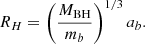
Now the rotation distribution can be constrained. As shown in Fig. 4, the rotation decay index α and the relative scale of core ${\overline{s}}_0$ is constrained in a narrow region. If α is considered to be three as suggested by Meyer & Meyer-Hofmeister (1979), ${\overline{s}}_0$ is about 0.02. The radius of the envelope can be obtained by the fallback time R_* ≃ 5 − 12 R_⊙ (Miniutti et al. 2023). Thus, the separation of the binary in the core is about 11 − 26 R_⊕. Wang et al. (2022) adopted the separation about 8.3 − 83 R_⊕ to estimate the eccentricity 0.97 − 1 by the Hills mechanism.

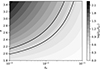Fig. 4. Constraint on the rotation decay index α and the relative scale of the core ${\overline{s}}_0$. The two solid lines represent (tp2/tp1)obs = 4.7 and 7.8. The area they enclose is the constrained region of the parameters.

As per the discussions in Sect. 2, the TDE occurs before the capture of the WD at the periastron. So $\widehat{v}$ is no longer perpendicular to ${\widehat{R}}_t$ when the envelope is disrupted. However, it only slightly affects the constraint on the rotation disruption. Detailed calculations are shown in Appendix A.

5. Discussion

While the tidal disruption of a CE can explain the second peak of the light curve of GSN 069, there is also a serious issue that the lifetime of a CE is very short, and the probability that we will see such events directly is very low. Simulations show that the maximum lifetime is only about 10⁵ times the orbital period of the binary in the core (Gagnier & Pejcha 2023). This timescale is only 273 years for a 1-day orbital period.

Another possibility is that the disrupted envelope is a circumbinary disk, which might be formed by the remaining material in the post-CE stage (Ivanova et al. 2013). If so, the circumbinary disk must not be a Keplerian disk, because it would be disrupted by a very slight tidal force.

To understand the detailed nature of the disrupted envelope, hydrodynamics simulations are necessary. Not only do the fallback rate curves need to take into account the interactions between the accreted material and the effect of the gravitation by the core and the captured WD, but also the realistic density and rotation distributions of the CE need to be simulated. If it can be confirmed that the TDE from GSN 069 is a disruption of the CE, then it is the closest one can get to a direct observation of the CE.

Our model also strongly relies on the validity of the binary model for QPEs following the capture of the star through the Hills mechanism. However, there are some alternative models for QPEs (Sniegowska et al. 2020; Ingram et al. 2021; Raj & Nixon 2021; Pan et al. 2022; Kaur et al. 2023). Future improvements in the understanding of the QPEs are very important for checking our model.

On the other hand, some other TDEs have a re-brightening peak (Jiang et al. 2019; Wevers et al. 2023; Malyali et al. 2023). Our model of the disruption of a differentially rotating envelope provides an alternative interpretation for such TDEs, even if they are not associated with QPEs. Not only does the envelope of the CE have differential rotation, but the envelope of the red giant may have it as well (Klion & Quataert 2017). Neither case necessarily requires the presence of QPEs. Considering the short lifetime of the CE. These sources are a little more likely to be the disruption of a red giant. Furthermore, our model can also produce a third peak if the disrupted envelope is in an eccentric orbit, which will make the binding energy of the stationary point further away from SMBH positive.

We cannot currently conclude whether these re-brightening TDEs are a disruption to the differentially rotating envelope because, as discussed in Sect. 4, only the time of the appearance of the second peak relative to the main peak is available for comparison with observations. Models that take into account density distributions, self-gravity, and gravity by the core may be able to provide more accurate fallback rate profiles that can be used to determine the nature of these re-brightening TDEs, which is beyond the scope of this Letter. Therefore, the study of more detailed models and numerical simulations is necessary in the future.

Acknowledgments

This work was supported by the National Key Research and Development Program of China (No. 2020YFC2201400) and National SKA Program of China (2020SKA0120300).

References

Appendix A: The disruption before reaching periastron

If the disruption occurs before the envelope reaches periastron, that is, β ≡ R_t/R_p > 1, $\widehat{v}$ is no longer perpendicular to ${\widehat{R}}_t$ when the envelope is disrupted. Assuming it rotates in the direction of ${\widehat{R}}_t$ by an angle γ, then Eq. 15 becomes

$$\begin{array}{c}\hfill ϵ={ϵ}_0\overline{s}(cos\varphi +k{\overline{s}}^{-\alpha }cos(\varphi +\gamma )).\end{array}$$(A.1)

For a parabolic orbit, γ can be obtained by

$$\begin{array}{c}\hfill sin\gamma =\frac{\sqrt{\beta }}{2}sinf,\end{array}$$(A.2)

where the true anomaly f is obtained by cos f = 2/β − 1.

As shown in Fig. A.1, the $\overline{ϵ}$ distribution with β = 10 is rotated compared with the distribution with β = 1. The position of the stationary point can be obtained by solving

$$\begin{array}{cc}\hfill \frac{\partial \overline{ϵ}}{\partial \overline{s}}& ={\overline{s}}^{-\alpha }[(1-\alpha )kcos(\varphi +\gamma )+{\overline{s}}^{\alpha }cos\varphi ]=0\hfill \\ \hfill \frac{\partial ϵ}{\overline{s}\partial \varphi }& =-k{\overline{s}}^{-\alpha }sin(\varphi +\gamma )-sin\varphi =0.\hfill \end{array}$$(A.3)

Fig. A.1. Same as Fig. 2, but with β = 10.

Then the time of the second peak can be obtained by the corresponding ϵ. As shown in the Fig. A.2, the constraint on the rotation distribution with β = 10 gives a slightly smaller α and a slightly larger $\overline{s}$ than those with β = 1.

Fig. A.2. Same as Fig. 4, but with β = 10.

All Figures

	Fig. 1. Value of the upper limit of Rt/RH for the companion star of various densities and masses. Here ρc and ρ* are the average density of the companion and the disrupted star, respectively. The solid line represents Rt/RH = 1.
In the text

	Fig. 2. Distribution of $\overline{ϵ}$ with k0 = 1, ${\overline{s}}_0=0.1$, and α = 3. The red star is the stationary point, and the corresponding $\overline{ϵ}$ is represented by the dashed line. The solid line represents $\overline{ϵ}=0$, and $\overline{ϵ}$ is negative on its left side and positive on its right side.
In the text

	Fig. 3. Fallback rate for the different rotation. Comparing the case of no rotation, the disruption of the envelope with differential rotation shows a second peak in the decay phase. The larger the core, the earlier the peak appears. The earlier fallback with differential rotation is caused by the innermost material, which has the lowest specific binding energy.
In the text

	Fig. 4. Constraint on the rotation decay index α and the relative scale of the core ${\overline{s}}_0$. The two solid lines represent (tp2/tp1)obs = 4.7 and 7.8. The area they enclose is the constrained region of the parameters.
In the text

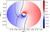	Fig. A.1. Same as Fig. 2, but with β = 10.
In the text

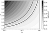	Fig. A.2. Same as Fig. 4, but with β = 10.
In the text

References

- Amaro-Seoane, P. 2018, Liv. Rev. Relat., 21, 4 [NASA ADS] [CrossRef] [Google Scholar]
- Arcodia, R., Merloni, A., Nandra, K., et al. 2021, Nature, 592, 704 [NASA ADS] [CrossRef] [Google Scholar]
- Chakraborty, J., Kara, E., Masterson, M., et al. 2021, ApJ, 921, L40 [NASA ADS] [CrossRef] [Google Scholar]
- Chen, X., Qiu, Y., Li, S., & Liu, F. 2022, ApJ, 930, 122 [NASA ADS] [CrossRef] [Google Scholar]
- Coughlin, E. R., & Nixon, C. 2019, ApJ, 883, L17 [NASA ADS] [CrossRef] [Google Scholar]
- Gagnier, D., & Pejcha, O. 2023, A&A, 674, A121 [NASA ADS] [CrossRef] [EDP Sciences] [Google Scholar]
- Gezari, S. 2021, ARA&A, 59, 21 [NASA ADS] [CrossRef] [Google Scholar]
- Giustini, M., Miniutti, G., & Saxton, R. D. 2020, A&A, 636, L2 [NASA ADS] [CrossRef] [EDP Sciences] [Google Scholar]
- Golightly, E. C., Coughlin, E. R., & Nixon, C. 2019, ApJ, 872, 163 [NASA ADS] [CrossRef] [Google Scholar]
- Hills, J. G. 1988, Nature, 331, 687 [Google Scholar]
- Ingram, A., Motta, S. E., Aigrain, S., & Karastergiou, A. 2021, MNRAS, 503, 1703 [NASA ADS] [CrossRef] [Google Scholar]
- Ivanova, N., Justham, S., Chen, X., et al. 2013, A&ARv, 21, 1 [CrossRef] [Google Scholar]
- Jiang, N., Wang, T., Mou, G., et al. 2019, ApJ, 871, 15 [Google Scholar]
- Kaur, K., Stone, N. C., & Gilbaum, S. 2023, MNRAS, 524, 1369 [Google Scholar]
- King, A. 2020, MNRAS, 493, L120 [Google Scholar]
- King, A. 2022, MNRAS, 515, 4344 [NASA ADS] [CrossRef] [Google Scholar]
- Klion, H., & Quataert, E. 2017, MNRAS, 464, L16 [NASA ADS] [CrossRef] [Google Scholar]
- Krolik, J. H., & Linial, I. 2022, ApJ, 941, 24 [NASA ADS] [CrossRef] [Google Scholar]
- Linial, I., & Metzger, B. D. 2023, ApJ, 957, 34 [NASA ADS] [CrossRef] [Google Scholar]
- Linial, I., & Sari, R. 2023, ApJ, 945, 86 [NASA ADS] [CrossRef] [Google Scholar]
- Lu, W., & Quataert, E. 2023, MNRAS, 524, 6247 [NASA ADS] [CrossRef] [Google Scholar]
- Malyali, A., Liu, Z., Rau, A., et al. 2023, MNRAS, 520, 3549 [NASA ADS] [CrossRef] [Google Scholar]
- Meng, X., & Podsiadlowski, P. 2017, MNRAS, 469, 4763 [NASA ADS] [CrossRef] [Google Scholar]
- Meyer, F., & Meyer-Hofmeister, E. 1979, A&A, 78, 167 [NASA ADS] [Google Scholar]
- Miniutti, G., Saxton, R., Giustini, M., et al. 2019, Nature, 573, 381 [NASA ADS] [CrossRef] [Google Scholar]
- Miniutti, G., Giustini, M., Arcodia, R., et al. 2023, A&A, 670, A93 [NASA ADS] [CrossRef] [EDP Sciences] [Google Scholar]
- Pan, X., Li, S.-L., Cao, X., Miniutti, G., & Gu, M. 2022, ApJ, 928, L18 [NASA ADS] [CrossRef] [Google Scholar]
- Raj, A., & Nixon, C. 2021, ApJ, 909, 82 [NASA ADS] [CrossRef] [Google Scholar]
- Sheng, Z., Wang, T., Ferland, G., et al. 2021, ApJ, 920, L25 [NASA ADS] [CrossRef] [Google Scholar]
- Shu, X., Wang, S., Dou, L., et al. 2018, ApJ, 857, L16 [NASA ADS] [CrossRef] [Google Scholar]
- Sniegowska, M., Czerny, B., Bon, E., & Bon, N. 2020, A&A, 641, A167 [NASA ADS] [CrossRef] [EDP Sciences] [Google Scholar]
- Song, J., Shu, X., Sun, L., et al. 2020a, A&A, 644, L9 [NASA ADS] [CrossRef] [EDP Sciences] [Google Scholar]
- Song, R., Meng, X., Podsiadlowski, P., & Cui, Y. 2020b, A&A, 633, A41 [NASA ADS] [CrossRef] [EDP Sciences] [Google Scholar]
- Suková, P., Zajaček, M., Witzany, V., & Karas, V. 2021, ApJ, 917, 43 [CrossRef] [Google Scholar]
- Wang, M., Yin, J., Ma, Y., & Wu, Q. 2022, ApJ, 933, 225 [NASA ADS] [CrossRef] [Google Scholar]
- Wevers, T., Coughlin, E., Pasham, D., et al. 2023, ApJ, 942, L33 [NASA ADS] [CrossRef] [Google Scholar]
- Xian, J., Zhang, F., Dou, L., He, J., & Shu, X. 2021, ApJ, 921, L32 [NASA ADS] [CrossRef] [Google Scholar]
- Zhao, Z., Wang, Y., Zou, Y., Wang, F., & Dai, Z. 2022, A&A, 661, A55 [NASA ADS] [CrossRef] [EDP Sciences] [Google Scholar]