| Issue |
A&A
Volume 688, August 2024
|
|
|---|---|---|
| Article Number | A74 | |
| Number of page(s) | 10 | |
| Section | Astrophysical processes | |
| DOI | https://doi.org/10.1051/0004-6361/202348071 | |
| Published online | 06 August 2024 | |
Solar wind data analysis aided by synthetic modeling: A better understanding of plasma frame variations from temporal data⋆
1
Centre for mathematical Plasma Astrophysics (CmPA), Department of Mathematics, KU Leuven, Celestijnenlaan 200B bus 2400, 3001 Leuven, Belgium
e-mail: norbert.magyar@kuleuven.be
2
Code 672, NASA, Goddard Space Flight Center, Greenbelt, MD 20771, USA
3
Section of Analysis, Department of Mathematics, KU Leuven, Celestijnenlaan 200B bus 2400, 3001 Leuven, Belgium
Received:
26
September
2023
Accepted:
19
May
2024
Context. In situ measurements of the solar wind, a turbulent and anisotropic plasma flow originating at the Sun, are mostly carried out by single spacecraft, resulting in one-dimensional time series.
Aims. The conversion of these measurements to the spatial frame of the plasma is a great challenge, but it is required for direct comparison of the measurements with magnetohydrodynamic turbulence theories.
Methods. We present a tool kit based on the synthetic modeling of solar wind fluctuations as two-dimensional noise maps with adjustable spectral and power anisotropy that can help with the temporal-spatial conversion of real data. Specifically, by following the spacecraft trajectory through a noise map (relative velocity and angle relative to some mean magnetic field) with properties tuned to mimic those of the solar wind, the likelihood that the temporal data fluctuations represent parallel or perpendicular fluctuations in the plasma frame can be quantified by correlating structure functions of the noise map. Synthetic temporal data can also be generated, which can provide a testing ground for analysis applied to the solar wind data.
Results. We demonstrate this tool by investigating Parker Solar Probe’s seventh encounter trajectory and data, and we showcase several possible ways in which it can be used. We find that whether temporal variations in the spacecraft frame come from parallel or perpendicular variations in the plasma frame strongly depends on the spectral and power anisotropy of the measured wind.
Conclusions. Data analysis assisted by such underlying synthetic models as presented here could open up new ways to interpret measurements in the future, specifically in the more reliable determination of plasma frame quantities from temporal measurements.
Key words: turbulence / methods: observational / Sun: heliosphere / solar wind
© The Authors 2024
 Open Access article, published by EDP Sciences, under the terms of the Creative Commons Attribution License (https://creativecommons.org/licenses/by/4.0), which permits unrestricted use, distribution, and reproduction in any medium, provided the original work is properly cited.
This article is published in open access under the Subscribe to Open model. Subscribe to A&A to support open access publication.
1. Introduction
The solar wind is a continuous supersonic and super-Alfvénic outflow of ionized particles (mostly protons and electrons) from the Sun driven partly by an as-of-yet undiscovered coronal heating mechanism (Klimchuk 2006; Arregui 2015; Van Doorsselaere et al. 2020) that renders the multi-million K solar corona unable to form (hydro)static equilibrium, as first shown by Parker (1958). Since the first experimental evidence of the solar wind provided by early satellites (Gringauz et al. 1960; Neugebauer & Snyder 1962), much effort has been devoted to understanding the measured fluctuations in velocity, magnetic field, and density, among other properties. It was soon realized that solar wind fluctuations display both turbulent (Coleman 1968) and Alfvén wave (Belcher & Davis 1971) characteristics on a large range of scales, the duality of which is thought to be the basis for understanding the nature of solar wind fluctuations, completed by the presence of advected non-Alfvénic and large-scale structures (Tu & Marsch 1995; Bruno & Carbone 2013, although see Borovsky 2020 for a different viewpoint). An important property of solar wind fluctuations is their anisotropy with respect to the local magnetic field direction, such as spectral, power, variance, and wavevector anisotropies (Horbury et al. 2012). Moreover, perpendicular fluctuations usually lack axisymmetry around the local magnetic field direction.
The interpretation of in situ data is complicated by the fact that most solar wind measurements rely on data from a single satellite or probe, that is, they represent single-point measurements along the relative plasma frame1 trajectory of the spacecraft. Therefore, the analysis of the provided one-dimensional temporal data requires a set of assumptions to be made for its re-interpretation as spatial data in the reference frame of the wind. This step is necessary in order to compare measurements to theoretical results that are given as functions of spatial variables or correlations. An almost universally applied assumption is Taylor’s hypothesis (Taylor 1938), which states that temporal variations in the spacecraft frame simply equal spatial variations in the plasma frame, t = −VSWx, where VSW is the solar wind speed vector. This can often be justified simply based on the observation that wind speeds are usually much faster than the characteristic velocity fluctuations and wave speeds in the plasma rest frame, rendering the fluctuations to appear “frozen” in the plasma as they are advected past the spacecraft. The Parker Solar Probe (PSP), launched in 2018, is the first satellite to enter the magnetically dominated solar corona, nearly three years after its launch (Kasper et al. 2021), and it continues to gather magnetic field and particle data, among other measurements, on successive encounters with perihelia as close to the solar surface as 10 R⊙. Recently, a considerable amount of work has been dedicated to studying the validity of Taylor’s hypothesis under various conditions, with the anticipation of PSP measurements for which the above inequality might not hold (e.g., Klein et al. 2014; Narita 2017; Bourouaine & Perez 2018; Chhiber et al. 2019; Perez et al. 2021), based on various phenomenological, analytical, or numerical models of solar wind turbulence. Uncertainties related to the interpretation of temporal data from PSP as spatial variations constitutes a motivation for applying the current analysis specifically to PSP data.
In studies of solar wind anisotropy, it is often assumed that for spacecraft trajectories in the plasma rest frame at shallow angles with respect to the local mean magnetic field (e.g., within 15°), the sampled measurements are of parallel (k∥) variations (Telloni et al. 2019). Various methods have been applied to solar wind measurements in order to reveal the anisotropy of the fluctuations as a function of the “angle of attack” of the spacecraft with respect to the local mean magnetic field. The spectral anisotropy of the solar wind fluctuation has been studied using wavelet analysis (e.g., by Horbury et al. 2008; Podesta 2009; Chen et al. 2011; Wang et al. 2016; Sakshee et al. 2022, to name a few) and Hilbert spectral analysis (Telloni et al. 2019), among other methods (Wang et al. 2015; Adhikari et al. 2022; Zhao et al. 2022), as a function of various conditions, such as intermittency, distance from the Sun, and the presence of switchbacks. Despite the large number of studies, there is still no consensus on the spectral anisotropy of the solar wind, even on the same data set, which illustrates the aforementioned difficulty in transforming temporal measurements into plasma frame data. Determining spectral anisotropy is important, for instance, because some theoretical works (Goldreich & Sridhar 1995) postulate the existence of critical balance in magnetohydrodynamic (MHD) turbulence, a manifestation of which are specific spectral power slopes along ( ) and across (
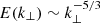 ) the local mean magnetic field, respectively. It is clear that a better knowledge of spatial variations of fluctuations would greatly advance our overall understanding of solar wind dynamics. For instance, a reliable determination of linear and nonlinear advective terms of the MHD equations in the solar wind could validate theories and phenomenologies of turbulence generation and evolution.
In this paper, we aim to assess the validity of interpreting temporal data as spatial plasma frame data through single-point solar wind measurements by developing a synthetic model of solar wind fluctuations. We consider the seventh encounter of PSP as the spacecraft trajectory through the synthetic model, with spacecraft speeds relative to the plasma frame and angles with respect to the local mean field given by PSP measurements. This allows for the direct comparison of the 1D synthetic temporal data in the spacecraft frame to the underlying synthetic spatial data. Among other tests, we explore the conditions under which the parallel or perpendicular fluctuations can be sampled depending on the degree of anisotropy; we test the limits of Taylor’s hypothesis; and we estimate the reliability in determining spatial gradients from temporal derivatives. The paper is organized as follows. In Sect. 2, we describe in detail the synthetic model employed. In Sect. 3, we describe the PSP data for the chosen encounter. In Sect. 4, we present several comparisons between the temporal and spatial data based on parametric studies of the synthetic model. Finally, in Sect. 5, we conclude with the results and discuss possible future applications and updates of the presented model.
2. Synthetic model
For the synthetic solar wind fluctuations, two-dimensional arrays were constructed using the numpy package (Harris et al. 2020) in Python. The choice of 2D arrays instead of 3D ones was made, on the one hand, based on the fact that the PSP orbit samples plasma in Venus’ orbital plane within an inclination of 4° to the Sun’s equator, with a negligible mean solar wind flow normal to this plane, and on the other hand, the choice was made for computational cost reduction. The fluctuations were constructed in the following way. An N2 2D array was populated with white noise (flat power spectrum) using the random.randn routine, which returns random floats sampled from a univariate normal (Gaussian) distribution. A real-valued filter was applied in k-space (element-wise multiplication) to the 2D FFT of the white noise array, which is an N2 2D array that determines the desired amplitudes and power spectral slopes for the k∥ and k⊥ directions, which are aligned with the principal axes of the matrix. There are multiple ways to construct such a filter. With the zero wave number at (N/2, N/2), that is, center-shifted spectrum, the positive valued k∥, k⊥ increase linearly toward the edges of the 2D array up to the Nyquist frequency and are symmetric across both principal axes. Here, we used N = 5000. The problem of finding a 2D filter with specified average power laws in the two directions is almost equivalent to the problem in probability theory of finding a joint distribution given two marginal distributions, where an integrability condition is further required. In the latter case, the standard procedure is to choose a copula function, which is the joint probability distribution with its two marginal distributions as the constant function on the interval [0, 1], and generate the desired joint distribution by taking inverse functions on the marginals. The simplest copula is the product copula, which assumes that the joint distribution is only the product of the two marginal distributions. In this case, the filter has the following form:
The product copula is highly anisotropic, having much less power in the oblique Fourier modes, thus resulting in very pronounced vertical and horizontal lines in real space. Since fluctuations are mostly spherically polarized in the solar wind (e.g., Vasquez & Hollweg 1998), it may be more realistic to consider a smoother (more isotropic) variation between the parallel and perpendicular directions while still resulting in the desired averaged spectra along these directions. Although more sophisticated copulas exist to yield such a result, they have more involved functional forms with tens of terms, including special functions, which may not be the most convenient choice for an application in our problem. Instead, we experimented with filters of the following form:
where A, B, C, α, β, and γ are constants that define the resulting 2D power spectrum. With F applied, we performed an inverse Fourier transform of the 2D array, resulting in an anisotropic colored noise 2D array, which we refer to in the following as the noise map. The power spectrum in the parallel and perpendicular directions was obtained by averaging 1D power spectra over all rows and columns of the noise map, respectively. This method of calculating parallel and perpendicular spectra is consistent with how these spectra are calculated for real data. Natural choices for parallel and perpendicular 1D power spectra and their ratios are the ones that were determined from in situ observations in previous works. Various studies of noise maps with different spectral and power anisotropies are presented in Sect. 5. Spectral anisotropy refers to different slope values for parallel and perpendicular power spectra, while power anisotropy refers to the ratio between perpendicular and parallel power (P⊥/P∥) at some specific scale, here chosen to be at the Nyquist frequency, that is, f = 0.5/cadence. If the spectral anisotropy is known, the power anisotropy of the noise maps can be calculated at any other scale based on this value. An example of a noise map and its parallel and perpendicular power spectra is illustrated in Fig. 1. Examples of some of the other noise maps used in this study are presented in Fig. 2. The constants used for noise maps with different power and spectral anisotropies are shown in Table 1.
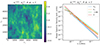 |
Fig. 1. Anisotropic 2D noise map (left) and its 1D Fourier power spectra averaged over all rows and columns (right). The term “PA” means “power anisotropy”, that is, the ratio of the power in the perpendicular to parallel wave number at the highest wave number. The terms r⊥ and r∥ are the array indices in the noise map perpendicular and parallel to the magnetic field, respectively. The amplitude of the noise map is shown in arbitrary units. |
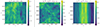 |
Fig. 2. Noise maps of different spectral and power anisotropies (PA), shown in the title of each map. The fluctuation amplitudes are in arbitrary units. |
3. Data description
We analyzed data from the seventh encounter of PSP, from January 13, 2021 00:00 UTC to January 22, 2021 00:00 UTC. The data are publicly available from CDAWeb2. From the FIELDS instrument suite (Bale et al. 2016), we used 3D fluxgate magnetometer data at four vectors/s in RTN coordinates, “mag_rtn_4_per_cycle”, and electron density measured through quasi-thermal noise. From the SWEAP (Kasper et al. 2016) instrument suite, we used proton data from the SPAN-I instrument (Livi et al. 2022) for velocity perturbations. We interpolated magnetic and density data to have the same cadence as velocity data, dt = 3.49 s. We applied the Butterworth filter (scipy.signal.butter of order five and critical frequency 0.03 in units of cadence) to the density data ρ in order to smooth its characteristic step-like instrumental oscillation without affecting the overall trend. The magnetic field data B was converted to velocity units b = Bρ−0.5. Average values of velocity and magnetic field in velocity units were calculated by means of moving average with a window size of 30 min. The Elsässer (1950) variables were calculated as
where sign(B0r) is the sign of the average radial magnetic field, assuring that the dominant outward-propagating Elsässer variable is z+, irrespective of the background magnetic field polarization. The full data for the analyzed duration are shown in Fig. 3. Next, we proceeded to calculate the angle between various vectors, such as the radial direction, average magnetic field, and relative velocity, given by the arc cosine of the dot product between the respective normalized vectors. The results are plotted in Fig. 4. The true angle of attack to the local mean magnetic field in the spacecraft frame is given by the angle between the relative velocity vector (VSC − VSW) and local average magnetic field direction. We note that in Fig. 4, most of the angle of attack variation is given by the variation of the average magnetic field direction superimposed on the weaker and longer trend represented by the angle between the relative spacecraft speed and the radial direction.
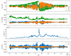 |
Fig. 3. In situ data from PSP showing (in RTN coordinates) the magnetic field, velocity, density, and normal component of Elsässer variables, respectively from top to bottom, during the analyzed time interval. |
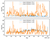 |
Fig. 4. Plots of the angle between the radial direction and 30-min moving average velocity and magnetic field direction (top graph) and the angle between the PSP velocity vector relative to the background flow(s) and the radial direction and average magnetic field direction (bottom graph) for the in situ PSP data shown in Fig. 3. |
4. Results
4.1. Gradient correlations of noise maps
Whether single-point measurements, as with PSP, measure the parallel or perpendicular fluctuations to some local magnetic field depends on the local solar wind speed, spacecraft speed, the variance, power, and spectral anisotropy of the perturbations as well as the angle of the local magnetic field direction with respect to the spacecraft trajectory in the plasma frame. The total derivative in the spacecraft’s frame of reference, equivalent to the derivative of spacecraft temporal data, is

where VSC and VSW are the spacecraft speed and the solar wind flow speed, respectively. The triad (R, T, N) represents the radial, tangential, normal coordinates, respectively, with R pointing toward the spacecraft from the Sun’s center, T = ω × R/|ω × R|, where ω is the Sun’s spin axis and N completes the right-handed triad. One way of estimating how well one can measure parallel or perpendicular fluctuations is by calculating the cross-correlation between the total derivative and the component-wise spatial derivatives as a function of angle of attack. The spatial derivative is proportional to the first-order structure function, defined by S1(r)=⟨[δf(r)]⟩, where δf(r)=f(R)−f(R + r), the difference of fluctuations at scale and direction r, where we have again neglected variation in the normal direction. We calculated the cross-correlations in the following way. First, we calculated 2D matrices obtained by shifting the noise maps along both axes by varying amounts and then subtracting the shifted matrix from the original. The purely parallel or perpendicular shifts were cross-correlated with matrices that had both parallel and perpendicular shifts, which represents the total derivative. The cross-correlation is defined as
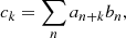
where a and b are the flattened matrices resulting in one-dimensional arrays, normalized such that the cross-correlation value is between [0, 1]:
where ⟨⟩ denotes the arithmetic mean, std is the standard deviation of the elements in x, and len(x) is the total number of elements in the x array. See Fig. 5 for cross-correlations between total and partial derivatives for a noise map with a specific spectral and power anisotropy. We repeated this procedure for noise maps of different spectral and power anisotropies, the latter being defined at the highest wave number and representing the limit of the MHD inertial range in the solar wind, around 500 km, which corresponds to the distance between two array elements in the noise maps. When investigating Fig. 5, it is clear that for the specific spectral and power anisotropy chosen, perpendicular variations are better correlated than parallel variations with the total derivative, except for smaller angles of attack of around 15° with respect to the magnetic field direction. We also note that the correlations decrease with increasing separation, both in the parallel and perpendicular directions, as the power anisotropy is scale dependent when there is a spectral anisotropy, which is the current case. In the case of no spectral anisotropy (k⊥ ∼ k∥ ∼ −5/3), power anisotropy is scale independent, and there is no decreasing correlation with distance, resulting in a considerably stronger perpendicular correlation overall.
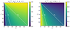 |
Fig. 5. Cross-correlation map of the total (dt) and perpendicular (left, ∂T) and total and parallel (right, ∂R) gradients for different r, ranging from zero to 60 in both perpendicular (r⊥) and parallel (r∥) directions. The unit distance corresponds to 500 km in the solar wind plasma frame. The title indicates the noise map used. The overplotted straight white lines of different slopes indicate different angles of attack. |
In Fig. 6, the power spectral slopes of the two noise maps with spectral anisotropy and different power anisotropies are shown as a function of the angle to the magnetic field direction. These curves were obtained by applying a rotation transform to the noise map by specific angles in increments of 5° from 0° to 90° and then averaging 1D spectra along the axes. Figure 6 can be compared to the similar plot of Horbury et al. (2008), derived from real solar wind data. The effect of power anisotropy on the variation of the slope with the angle is in agreement with the correlation plots: larger power anisotropy makes it more difficult to measure parallel variations. It is interesting to note that the true perpendicular spectrum is only attained for perpendicular trajectories, and there seems to be no constant plateau after some angle, contrary to what observational analysis suggests in Horbury et al. (2008). In the case of the noise maps, the transitional curve between parallel and perpendicular spectra is determined by the shape of the copula in Eq. (2). Understanding the physical origins of such transitional curves determined from observational data might reveal the physics of solar wind fluctuations.
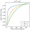 |
Fig. 6. Slopes of average 1D power spectra as a function of the angle to the magnetic field direction for the noise maps with spectral anisotropy for different power anisotropies. |
4.2. Application to PSP measurements
Based on the measured angle of attack values and by assuming a specific power and spectral anisotropy of the noise map that best matches the spectral properties of the solar wind, it is possible to make various predictions concerning the real data. For example, one can estimate the likelihood that measured perturbations represent parallel or perpendicular variations in the plasma frame based on the cross-correlation maps in Fig. 5. Within this section, we mostly showcase the various analyses possible using this tool kit by employing a noise map with spectral anisotropy (k⊥ ∼ −5/3; k∥ ∼ −2) and a power anisotropy of seven. Thus, findings based on this noise map are only valid as long as the spectral properties of the noise map approximate well those of the solar wind. We do not claim that the chosen spectral and power anisotropy of the noise map is the representative or typical spectral and power anisotropy of the solar wind fluctuations for this particular PSP encounter. Caveats of choosing a single noise map for the whole duration of the encounter and of these particular values of spectral and power anisotropy are discussed in Sect. 5. Calculating the spatial distance in the plasma frame as the relative speed multiplied by the cadence, one can assign a normalized correlation value to each pair of measured angle of attack and distance values, shown in Fig. 7 for the noise map in Fig. 1.
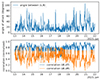 |
Fig. 7. Measured angle of attack to the local mean magnetic field (top) and the corresponding normalized cross-correlation coefficient between the total and radial (parallel) and total and tangential (perpendicular) derivatives (bottom). |
The mean plasma frame distance between two measurements with the present cadence is 1350 km (minimum 740 km, maximum 2370 km), which corresponds to a mean power anisotropy of six (minimum 5, maximum 6.8) in the noise map of Fig. 1. Looking at Fig. 7, it is again clear that most of the temporal variation in the spacecraft frame is given by perpendicular variations in the plasma frame for a noise map with spectral anisotropy and a power anisotropy of seven. The statistics of correlations are shown in Fig. 8 also for the other noise maps in Table 1.
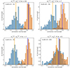 |
Fig. 8. Histograms with the distribution of correlation coefficients obtained by scanning through the correlation maps with the angles of attack obtained from PSP measurements using a mean field with a moving average of 30 min. The specific spectral and power anisotropies are shown at the top of each histogram plot. The orange (blue) bars represent the perpendicular (parallel) correlations, and the vertical lines represent the mean value of the correlation for the entire encounter period analyzed. Also shown is the percentage of points for which the parallel correlation value is higher than the perpendicular one. |
The dominance of plasma frame perpendicular variations in the spacecraft frame temporal variation increases with increasing power anisotropy and with decreasing spectral anisotropy. As such, for a power anisotropy of seven, there is a dominance of perpendicular variations in the temporal variation, with the parallel variation having a better correlation only 9% of the time. For a power anisotropy of five, the average correlation values with parallel and perpendicular variations are very close, meaning that in this case, high correlations with either parallel or perpendicular variations are only achievable for nearly parallel or perpendicular angles of attack, respectively.
Using the correlation values shown in Fig. 7 calculated specifically for the PSP measurements, it is possible to statistically study various plasma frame quantities derived from the PSP measurements while being able to assign a value to how accurately these measurements represent parallel or perpendicular variations. In the following, we show the example of a linear and nonlinear advection study based on data points for which either the perpendicular or parallel correlations are above 0.8, thus showing a very good correlation. The noise map used is the same as in Fig. 1, and thus the number of points satisfying the larger than 0.8 correlation criterion is much higher for perpendicular correlations than parallel ones. Still, there seem to be enough parallel correlation points (≈5000) for a statistical study. In Fig. 9, the linear advection, measured for high parallel correlation, and the nonlinear advection, measured for high perpendicular correlation, are shown. The perturbations are rotated to a reference frame pointing in the relative direction of the spacecraft velocity in the plasma frame, which is almost identical to the radial direction in the case of high parallel correlation. In this sense, the calculated advection represents a component of the total advection vector, with a weight of almost 100% for linear advection and around 50% for nonlinear advection. It is important to keep in mind that the linear and nonlinear advection calculated in this way are not for the same plasma element, as high parallel or perpendicular correlation regions do not overlap. The plots in Fig. 9 show that linear advection is higher for the dominant Elsässer variable (here z+), as expected. The nonlinear advection for z± are of the same magnitude, implying that nonlinear advection is relatively more important for the minority Elsässer variable (here z−). It appears that by taking into account that the calculated nonlinear advection component is on average 50% of the total value, the linear and nonlinear advection have around the same values for z−, while the nonlinear advection is around half the linear advection for z+. Thus, the advection of z− appears to be in critical balance, while z+ could be in critical balance for short intervals, possibly in an intermittent manner.
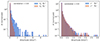 |
Fig. 9. Histograms showing the absolute value of the calculated linear advection (left) and nonlinear advection (right) for correlations above 0.8 with parallel or perpendicular variations, respectively. The calculated advection represents the component in the direction of the spacecraft velocity relative to the local plasma frame. Advection terms have been calculated for both Elsässer variables. |
Another example of how synthetic data can be of help in understanding one-point spacecraft measurements is the following. It is possible to extract synthetic perturbations through the noise map by simulating a PSP fly-through of the noise map, with background wind speed, spacecraft speed, and angle of attack given by PSP measurements. This is shown in Fig. 10. The angle of attack variation can be simulated by multiplying the relative velocity components of the spacecraft with the cosine and sine of the measured angle values. Then, synthetic measurements can be obtained by extracting data points from the noise map along the simulated PSP trajectory. The generation of synthetic velocity or magnetic field perturbation vectors with three components is possible by using a different noise map for each component. For example, magnetic field perturbations with a constant magnitude, that is, zero compressibility or spherical polarization, can be constructed by generating two different random noise maps for the tangential and normal components, for example, and by defining the radial component as
 |
Fig. 10. Polar plot showing the ecliptic plane in the HCI frame with the PSP orbit during the seventh encounter (here shown from 13 to 21 January 2021). The trajectory is depicted with a white curve. The background is given by the noise map in Fig. 1. The radial distance is in units of solar radii. An animation of this figure is available online. |
where the max() finds the maximal value within a specific array. We note that in this case, the radial magnetic field is always positive, thus no synthetic magnetic switchbacks that flip the magnetic field polarization are present. An example of synthetic magnetic field perturbation time series constructed in such a way is shown in Fig. 11. Using such synthetic 1D measurements, the analysis presented earlier can be repeated, such as the correlation between the gradient of the synthetic 1D measurement and the spatial gradients at the location of the spacecraft. Correlations derived in such a way show a very good agreement with the correlations derived directly from correlation maps (Fig. 7), with some fluctuations that change for each set of random numbers used to generate the noise map. The power spectrum of the synthetic 1D fluctuations can also be analyzed, with the power spectrum for the total duration and the noise map in Fig. 1 shown in Fig. 12. The variance anisotropy (difference in amplitude between parallel and perpendicular components of the synthetic perturbations) is around 15, which is in the upper range of previously reported variance anisotropies in real data, where the typical values are around six (e.g., Smith et al. 2006) and nine, as reported by Belcher & Davis (1971). The measured total power spectral slope is close to −5/3, indicating yet again the dominance of the perpendicular variations in the temporal data. We have conducted a wavelet analysis as well in order to study the angle of attack-dependent power spectra of the synthetic data, with similar parameters to the one presented in Horbury et al. (2008). The result is shown in Fig. 13. The wavelet technique applied to the synthetic 1D data shows a very good agreement with the one derived through rotating the noise map and then averaging the spectra over all 1D lines, also shown Fig. 6. In the future, it would be of interest to perform all other analysis techniques that were used to disentangle parallel and perpendicular spectra (e.g., Hilbert spectral analysis Telloni et al. 2019) to see if different results are obtained.
 |
Fig. 11. Synthetic magnetic field perturbations derived from the noise map shown in Fig. 1 showing each component and the total magnitude, which is constant. |
 |
Fig. 12. Power spectral density for the three synthetic components of the magnetic field for the whole duration of the analyzed PSP encounter. Also shown is a moving average of the tangential component for easier comparison to the overplotted −5/3 slope. |
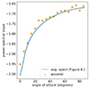 |
Fig. 13. Angle of attack-dependent spectra calculated in two different ways. In one approach, the calculation was performed by averaging over the spectra of 1D lines at a specific angle to the noise map principal axes (also shown in Fig. 6); the second approach involved applying the wavelet technique as described in Horbury et al. (2008) to the synthetic 1D data. |
As a final example of the applicability of the synthetic maps, one could also use the synthetic data to determine the limit of validity of Taylor’s hypothesis by considering local deformations of the noise map along the followed trajectory. Then, the unaltered signal (i.e., “frozen-in” fluctuations) can be correlated with the signal suffering deformations proportional to some deformation constant τ. The results are shown in Fig. 14. The deformation constant can be interpreted as the inverse of some deformation time normalized to the cadence, with its value reflecting the relative amount of advection or deformation suffered by fluctuations in the plasma frame, where a value of τ = 1 represents deformation on the order of the fluctuations. This can be taken to be equivalent to the ratio of the velocity fluctuation amplitude in the plasma rest frame (δv) to the spacecraft speed relative to this frame (V⊥) in the perpendicular direction to the magnetic field, τ = δv/V⊥. In this sense, τ is proportional to the quantity ϵ used in Perez et al. (2021). We note that using ϵ as defined in Perez et al. (2021) would lead to highly varying “deformation” rates, as the angle of attack varies greatly. Instead, for demonstrative purposes, we opted for a steady or average rate of deformation over time as quantified by the value of τ. Thus, τ here can be interpreted as an average ϵ multiplied by  . The deformations are introduced by Fourier transforming a square region around the measurement point in the noise map (10 pixels, or 5000 km wide) and rotating (phase shifting) the resulting complex k-plane by a different random amount at each discrete (k⊥, k∥). The maximum allowed rotation is then given by τ in units of a full rotation (2π). We note that the random numbers scale as k, as the deformation time is proportional to the scale of the fluctuations. Thus, higher frequencies are deformed faster. The k = 0 mode is not rotated, and thus there is no change in the mean value of the deformed square. The square is then inverse Fourier-transformed to obtain the locally deformed state of the noise map. There are two main observations to be made by looking at Fig. 14. First, the correlation clearly decreases as the deformation time decreases, or equivalently, as τ increases. Second, the impact of the background flow speed is very visible; the correlation is higher for higher wind speeds before perihelion (13 to 17 January; see background wind speed in Fig. 3). While there is still some correlation remaining for τ = 1 (i.e., deformation on the order of the amplitude of the fluctuations), this is mostly due to the larger scales that remain better correlated. Thus, besides the wind speed, the linear and nonlinear deformation time has a strong influence on the validity of Taylor’s hypothesis. The impact of the deformation on the power spectrum was also checked, and we found no impact on the overall spectrum. This is understandable, as the deformations only impacted the phase of the fluctuations.
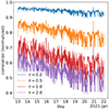 |
Fig. 14. Correlation between the 1D synthetic data extracted from an unchanging “frozen-in” noise map and the noise map undergoing deformations of a magnitude set by τ for the whole analyzed period of the encounter. |
5. Conclusions
Most of our understanding of solar wind dynamics comes from single spacecraft measurements, which provide magnetic field or particle data, or both, at some specified temporal cadence. The Parker Solar Probe is one recent example of a spacecraft providing such measurements. However, the solar wind is a three-dimensional anisotropic plasma flow displaying strong fluctuations, with a mean magnetic field strongly varying in direction spatially and with different properties along and across the mean field, a fact also predicted by several theoretical studies. In this sense, it is a great challenge to transform the temporal data of the spacecraft into the spatial plasma frame that is better suited to theoretical scrutiny. Even with Taylor’s hypothesis being valid, separating between parallel and perpendicular spatial variations is not straightforward. Even more worrisome, in regions scanned by PSP closer to the Sun, the validity of Taylor’s hypothesis is questionable.
Initially motivated by attempting to determine the nonlinear advection term from solar wind measurements, we have devised a tool for approximating the likelihood that temporal measurements represent either parallel or perpendicular variations in the plasma frame with the help of synthetic anisotropic 2D noise maps. These noise maps can be constructed with specific power and spectral anisotropies, ideally ones that match with the studied solar wind period. Although determining the power and spectral anisotropies of solar wind data is a challenge in the first place – and thought to depend on a number of solar wind parameters – average representative values can be used for this purpose. More specifically, there is an ongoing debate as to the conditions fluctuations parallel to the local mean magnetic field scale as k−2 or k−5/3. Therefore, we have analyzed multiple noise maps with different power and spectral anisotropies.
The likelihood that the temporal variations represent parallel or perpendicular variations in the plasma frame was determined by calculating the first-order structure functions (proportional to spatial gradients) from the noise maps and then correlating these with either their perpendicular or parallel components. These correlation maps then assigned a correlation coefficient, normalized between zero and one, between the total derivative and parallel or perpendicular derivatives, depending on the spatial distance between two measurements and the angle between the local mean magnetic field and the relative velocity vector of the spacecraft in the plasma frame, referred to as the “angle of attack”.
Then, given the real measurements of the plasma frame distance between two data points, calculated from relative speed multiplied by the cadence, and the angle of attack, calculated as the angle between the local mean magnetic field and the relative velocity vector of the spacecraft, we assigned perpendicular and parallel correlation values to each measurement point, which can be used to select intervals with likely high perpendicular or parallel correlation. The immediate outcome of this study is that power anisotropy and, to a lesser degree, spectral anisotropy have a strong effect on whether the measured temporal data comes from perpendicular or parallel variations in the plasma frame. The most important role is played by power anisotropy, as a larger anisotropy leads to a higher correlation between the temporal and perpendicular variations. Spectral anisotropy renders power anisotropy scale dependent, decreasing it at larger scales and therefore indirectly having an impact on the correlations. For a noise map with spectral anisotropy of  and power anisotropy at the high frequency end of the inertial range of seven, most of the temporal variation is given by perpendicular variations in the noise map. A good correlation (≥0.8) with parallel variations is only encountered in 9% of the total duration of PSP’s seventh solar encounter. Without spectral anisotropy, the same power anisotropy would only have a good parallel correlation 4% of the time.
We have presented some other applications of the synthetic maps to aid in data analysis. Linear and nonlinear advection were calculated for intervals with good parallel and perpendicular correlations, respectively. These might indicate the advection of the minority Elsässer variable being critically balanced, while the majority Elsässer variable possibly only satisfies critical balance intermittently, being on average half the value of linear advection.
Synthetic measurements can also be constructed for multiple components of perturbations based on the noise maps, including ones with spherical polarization or constant perturbation vector magnitude. These measurements are extracted from the noise map along the same trajectory (distance and angle of attack) as measured by PSP. The synthetic measurements obtained in such a way can be subjected to the same analysis methods as real data, with the advantage of also knowing their spatial variation. As such, we obtained power spectra for the whole encounter duration of the synthetic data, showing a spectral slope close to −5/3. In order to reveal the parallel scaling, we applied the same wavelet analysis as employed by Horbury et al. (2008) to the synthetic data, revealing the angle of attack-dependent spectra of the noise map for the trajectory, which agrees well with the angle of attack-dependent spectral slope obtained directly from averaging the noise map spectra. Synthetic measurements of this kind could be a tool to test and validate analysis methods applied to real data. Finally, we tested Taylor’s hypothesis by inducing localized deformations of the noise map along the relative spacecraft trajectory. By correlating the synthetic measurement from the nondeformed (static) noise map with the one from the deformed noise map, an upper limit of the linear or nonlinear timescale can be determined, for which Taylor’s hypothesis is still valid. The correlation increases with wind speed, as expected. The correlation is still good (≥0.8) for the seventh encounter of PSP up to a relative deformation of τ = 0.5 amplitudes at the smallest scales within one cadence duration.
There are a number of caveats regarding this study. First of all, the validity of various analyses based on the noise map as presented above is directly tied to how well the spectral and power anisotropy of the chosen noise map approximates that of the solar wind. As these properties of the solar wind are highly variable (e.g., Zhao et al. 2022), care should be taken when choosing any single noise map to be representative for the whole interval analyzed. We chose the same noise map for the whole interval with specific spectral and power anisotropies in order to demonstrate the capabilities of this tool kit. Additionally, the dimensionality of the noise map could be made 3D for a fully replicated trajectory and to further allow for asymmetry between the two perpendicular directions. Furthermore, the dimensions of the noise map could be increased, which would allow for the extraction of more synthetic data points, increasing the statistical significance of the performed analysis. Second, the noise maps used do not display intermittency as turbulence in the solar wind does. Intermittency is known to be very relevant for the determination of power and spectral anisotropy in solar wind measurements (Wang et al. 2014). This could be improved by using random distributions with some specified kurtosis when generating the noise maps. The results of full 3D MHD simulations, which result self-consistently in anisotropic and intermittent turbulent fluctuations, have been used previously for such purposes. However, in the case of simulation data, the power and spectral anisotropies are not configurable but are the result of the dynamics; therefore, no parametric studies on the impact of these properties is possible. Additionally, the obtained synthetic measurements do not display the 1/r2 decrease in average magnetic field magnitude with distance from the Sun or heliospheric current sheet crossings. These could be included by modulating the fluctuations by the measured large-scale mean magnetic field.
A necessary future extension of this study would be the constraining and updating of the noise map properties by the measured average properties of the wind that is being analyzed. For example, in Zhao et al. (2022), Sioulas et al. (2023), it is shown that both the measured power and spectral anisotropy change with distance from the Sun, with spectral anisotropy even being scale dependent, as also noted recently by Telloni (2022), Wu et al. (2023). Updated noise maps should take all of these observations into account. Additionally, the influence of the violation of Taylor’s hypothesis on the anisotropy measurements could also be thoroughly tested in the future by deforming noise maps, as presented here.
In summary, by generating and analyzing synthetic data based on noise maps with properties mimicking the properties of turbulence in the solar wind we can gain better insights into solar wind dynamics. More specifically, it could help in understanding the interplay between the temporal measurements in the spacecraft frame and spatial variations in the plasma frame, which would allow for a better comparison between observations and turbulence theories.
Movie
Movie 1 associated with Fig. 10 Access here
Acknowledgments
N.M. acknowledges Research Foundation – Flanders (Fonds voor Wetenschappelijk Onderzoek – Vlaanderen) for their support through a Postdoctoral Fellowship. This research was supported by the International Space Science Institute (ISSI) in Bern, through ISSI International Team project #560: “Turbulence at the Edge of the Solar Corona: Constraining Available Theories Using the Latest Parker Solar Probe Measurements”. J.V. acknowledges support from NASA PSP-GI 80NSSC23K0208. T.V.D. was supported by the European Research Council (ERC) under the European Union’s Horizon 2020 research and innovation programme (grant agreement No. 724326) and the C1 grant TRACEspace of Internal Funds KU Leuven. T.V.D. has benefited from the funding of the FWO Vlaanderen through a Senior Research Project (G088021N).
References
- Adhikari, L., Zank, G. P., Zhao, L. L., & Telloni, D. 2022, ApJ, 933, 56 [NASA ADS] [CrossRef] [Google Scholar]
- Arregui, I. 2015, Philos. Trans. R. Soc. London Ser. A, 373, 20140261 [Google Scholar]
- Bale, S. D., Goetz, K., Harvey, P. R., et al. 2016, Space Sci. Rev., 204, 49 [Google Scholar]
- Belcher, J. W., & Davis, L. 1971, J. Geophys. Res., 76, 3534 [Google Scholar]
- Borovsky, J. E. 2020, Front. Astron. Space Sci., 7, 20 [NASA ADS] [CrossRef] [Google Scholar]
- Bourouaine, S., & Perez, J. C. 2018, ApJ, 858, L20 [Google Scholar]
- Bruno, R., & Carbone, V. 2013, Liv. Rev. Sol. Phys., 10, 2 [Google Scholar]
- Chen, C. H. K., Mallet, A., Yousef, T. A., Schekochihin, A. A., & Horbury, T. S. 2011, MNRAS, 415, 3219 [Google Scholar]
- Chhiber, R., Usmanov, A. V., Matthaeus, W. H., Parashar, T. N., & Goldstein, M. L. 2019, ApJS, 242, 12 [Google Scholar]
- Coleman, P. J. 1968, ApJ, 153, 371 [Google Scholar]
- Elsässer, W. M. 1950, Phys. Rev., 79, 183 [CrossRef] [Google Scholar]
- Goldreich, P., & Sridhar, S. 1995, ApJ, 438, 763 [Google Scholar]
- Gringauz, K. I., Bezrokikh, V. V., Ozerov, V. D., & Rybchinskii, R. E. 1960, Sov. Phys. Dokl., 5, 361 [NASA ADS] [Google Scholar]
- Harris, C. R., Millman, K. J., van der Walt, S. J., et al. 2020, Nature, 585, 357 [NASA ADS] [CrossRef] [Google Scholar]
- Horbury, T. S., Forman, M., & Oughton, S. 2008, Phys. Rev. Lett., 101, 175005 [Google Scholar]
- Horbury, T. S., Wicks, R. T., & Chen, C. H. K. 2012, Space Sci. Rev., 172, 325 [Google Scholar]
- Kasper, J. C., Abiad, R., Austin, G., et al. 2016, Space Sci. Rev., 204, 131 [Google Scholar]
- Kasper, J. C., Klein, K. G., Lichko, E., et al. 2021, Phys. Rev. Lett., 127, 255101 [NASA ADS] [CrossRef] [Google Scholar]
- Klein, K. G., Howes, G. G., & TenBarge, J. M. 2014, ApJ, 790, L20 [Google Scholar]
- Klimchuk, J. A. 2006, Sol. Phys., 234, 41 [Google Scholar]
- Livi, R., Larson, D. E., Kasper, J. C., et al. 2022, ApJ, 938, 138 [NASA ADS] [CrossRef] [Google Scholar]
- Narita, Y. 2017, Ann. Geophys., 35, 325 [Google Scholar]
- Neugebauer, M., & Snyder, C. W. 1962, Science, 138, 1095 [Google Scholar]
- Parker, E. N. 1958, ApJ, 128, 664 [Google Scholar]
- Perez, J. C., Bourouaine, S., Chen, C. H. K., & Raouafi, N. E. 2021, A&A, 650, A22 [EDP Sciences] [Google Scholar]
- Podesta, J. J. 2009, ApJ, 698, 986 [NASA ADS] [CrossRef] [Google Scholar]
- Sakshee, S., Bandyopadhyay, R., & Banerjee, S. 2022, MNRAS, 514, 1282 [NASA ADS] [CrossRef] [Google Scholar]
- Sioulas, N., Velli, M., Huang, Z., et al. 2023, ApJ, 951, 141 [CrossRef] [Google Scholar]
- Smith, C. W., Vasquez, B. J., & Hamilton, K. 2006, J. Geophys. Res.: Space Phys., 111, A09111 [NASA ADS] [Google Scholar]
- Taylor, G. I. 1938, Proc. R. Soc. London Ser. A, 164, 476 [Google Scholar]
- Telloni, D. 2022, Front. Astron. Space Sci., 9, 917393 [NASA ADS] [CrossRef] [Google Scholar]
- Telloni, D., Carbone, F., Bruno, R., et al. 2019, ApJ, 887, 160 [Google Scholar]
- Tu, C.-Y., & Marsch, E. 1995, Space Sci. Rev., 73, 1 [Google Scholar]
- Van Doorsselaere, T., Srivastava, A. K., Antolin, P., et al. 2020, Space Sci. Rev., 216, 140 [Google Scholar]
- Vasquez, B. J., & Hollweg, J. V. 1998, J. Geophys. Res., 103, 335 [NASA ADS] [CrossRef] [Google Scholar]
- Wang, X., Tu, C., He, J., Marsch, E., & Wang, L. 2014, ApJ, 783, L9 [NASA ADS] [CrossRef] [Google Scholar]
- Wang, X., Tu, C., He, J., et al. 2015, ApJ, 810, L21 [NASA ADS] [CrossRef] [Google Scholar]
- Wang, X., Tu, C., Marsch, E., He, J., & Wang, L. 2016, ApJ, 816, 15 [NASA ADS] [CrossRef] [Google Scholar]
- Wu, H., He, J., Huang, S., et al. 2023, ApJ, 947, 45 [NASA ADS] [CrossRef] [Google Scholar]
- Zhao, L. L., Zank, G. P., Adhikari, L., & Nakanotani, M. 2022, ApJ, 924, L5 [NASA ADS] [CrossRef] [Google Scholar]
All Tables
All Figures
|
Fig. 1. Anisotropic 2D noise map (left) and its 1D Fourier power spectra averaged over all rows and columns (right). The term “PA” means “power anisotropy”, that is, the ratio of the power in the perpendicular to parallel wave number at the highest wave number. The terms r⊥ and r∥ are the array indices in the noise map perpendicular and parallel to the magnetic field, respectively. The amplitude of the noise map is shown in arbitrary units. |
| In the text | |
|
Fig. 2. Noise maps of different spectral and power anisotropies (PA), shown in the title of each map. The fluctuation amplitudes are in arbitrary units. |
| In the text | |
|
Fig. 3. In situ data from PSP showing (in RTN coordinates) the magnetic field, velocity, density, and normal component of Elsässer variables, respectively from top to bottom, during the analyzed time interval. |
| In the text | |
|
Fig. 4. Plots of the angle between the radial direction and 30-min moving average velocity and magnetic field direction (top graph) and the angle between the PSP velocity vector relative to the background flow(s) and the radial direction and average magnetic field direction (bottom graph) for the in situ PSP data shown in Fig. 3. |
| In the text | |
|
Fig. 5. Cross-correlation map of the total (dt) and perpendicular (left, ∂T) and total and parallel (right, ∂R) gradients for different r, ranging from zero to 60 in both perpendicular (r⊥) and parallel (r∥) directions. The unit distance corresponds to 500 km in the solar wind plasma frame. The title indicates the noise map used. The overplotted straight white lines of different slopes indicate different angles of attack. |
| In the text | |
|
Fig. 6. Slopes of average 1D power spectra as a function of the angle to the magnetic field direction for the noise maps with spectral anisotropy for different power anisotropies. |
| In the text | |
|
Fig. 7. Measured angle of attack to the local mean magnetic field (top) and the corresponding normalized cross-correlation coefficient between the total and radial (parallel) and total and tangential (perpendicular) derivatives (bottom). |
| In the text | |
|
Fig. 8. Histograms with the distribution of correlation coefficients obtained by scanning through the correlation maps with the angles of attack obtained from PSP measurements using a mean field with a moving average of 30 min. The specific spectral and power anisotropies are shown at the top of each histogram plot. The orange (blue) bars represent the perpendicular (parallel) correlations, and the vertical lines represent the mean value of the correlation for the entire encounter period analyzed. Also shown is the percentage of points for which the parallel correlation value is higher than the perpendicular one. |
| In the text | |
|
Fig. 9. Histograms showing the absolute value of the calculated linear advection (left) and nonlinear advection (right) for correlations above 0.8 with parallel or perpendicular variations, respectively. The calculated advection represents the component in the direction of the spacecraft velocity relative to the local plasma frame. Advection terms have been calculated for both Elsässer variables. |
| In the text | |
|
Fig. 10. Polar plot showing the ecliptic plane in the HCI frame with the PSP orbit during the seventh encounter (here shown from 13 to 21 January 2021). The trajectory is depicted with a white curve. The background is given by the noise map in Fig. 1. The radial distance is in units of solar radii. An animation of this figure is available online. |
| In the text | |
|
Fig. 11. Synthetic magnetic field perturbations derived from the noise map shown in Fig. 1 showing each component and the total magnitude, which is constant. |
| In the text | |
|
Fig. 12. Power spectral density for the three synthetic components of the magnetic field for the whole duration of the analyzed PSP encounter. Also shown is a moving average of the tangential component for easier comparison to the overplotted −5/3 slope. |
| In the text | |
|
Fig. 13. Angle of attack-dependent spectra calculated in two different ways. In one approach, the calculation was performed by averaging over the spectra of 1D lines at a specific angle to the noise map principal axes (also shown in Fig. 6); the second approach involved applying the wavelet technique as described in Horbury et al. (2008) to the synthetic 1D data. |
| In the text | |
|
Fig. 14. Correlation between the 1D synthetic data extracted from an unchanging “frozen-in” noise map and the noise map undergoing deformations of a magnitude set by τ for the whole analyzed period of the encounter. |
| In the text | |
Current usage metrics show cumulative count of Article Views (full-text article views including HTML views, PDF and ePub downloads, according to the available data) and Abstracts Views on Vision4Press platform.
Data correspond to usage on the plateform after 2015. The current usage metrics is available 48-96 hours after online publication and is updated daily on week days.
Initial download of the metrics may take a while.