| Issue |
A&A
Volume 682, February 2024
|
|
|---|---|---|
| Article Number | A1 | |
| Number of page(s) | 19 | |
| Section | Stellar structure and evolution | |
| DOI | https://doi.org/10.1051/0004-6361/202347991 | |
| Published online | 26 January 2024 | |
First spectroscopic investigation of anomalous Cepheid variables⋆
1
INAF – Osservatorio Astronomico di Capodimonte, Salita Moiariello 16, 80131 Naples, Italy
e-mail: vincenzo.ripepi@inaf.it
2
INAF – Osservatorio Astrofisico di Catania, Via S. Sofia 78, 95123 Catania, Italy
3
Leibniz – Institut für Astrophysik Potsdam (AIP), An der Sternwarte 16, 14482 Potsdam, Germany
4
Institut für Physik und Astronomie, Universität Potsdam, Haus 28, Karl-Liebknecht-Str. 24/25, 14476 Golm, (Potsdam), Germany
5
Istituto Nazionale di Astrofisica – Osservatorio Astronomico d’Abruzzo, Via M. Maggini s.n.c., 64100 Teramo, Italy
6
Istituto Nazionale di di Fisica Nucleare – sezione di Roma, Piazzale Aldo Moro 2, 00185 Roma, Italy
7
Dipartimento di Fisica e Astronomia “Augusto Righi”, Alma Mater Studiorum, Universitá di Bologna, Via Gobetti 93/2, 40129 Bologna, Italy
8
INAF – Osservatorio di Astrofisica e Scienza dello Spazio di Bologna, Via Gobetti 93/3, 40129 Bologna, Italy
9
INAF – Osservatorio Astronomico di Roma, Via Frascati 33, 00078 Monte Porzio Catone, Italy
10
IAC – Instituto de Astrofísica de Canarias, Calle Vía Lactea s/n, 38205 La Laguna, Tenerife, Spain
11
Departmento de Astrofísica, Universidad de La Laguna, 38206 La Laguna, Tenerife, Spain
12
Istituto Nazionale di Fisica Nucleare (INFN)-Sez. di Napoli, Via Cinthia, 80126 Napoli, Italy
Received:
16
September
2023
Accepted:
30
October
2023
Context. Anomalous Cepheids (ACEPs) are intermediate-mass metal-poor pulsators that are mostly discovered in dwarf galaxies of the Local Group. However, recent Galactic surveys, including the Gaia Data Release 3, found a few hundred ACEPs in the Milky Way. Their origin is only poorly understood.
Aims. We aim to investigate the origin and evolution of Galactic ACEPs by studying the chemical composition of their atmospheres for the first time.
Methods. We used UVES at the Very Large Telescope to obtain high-resolution spectra for a sample of nine ACEPs belonging to the Galactic halo. We derived the abundances of 12 elements, C, Na, Mg, Si, Ca, Sc, Ti, Cr, Fe, Ni, Y, and Ba. We complemented these data with literature abundances from high-resolution spectroscopy for an additional three ACEPs that were previously incorrectly classified as type II Cepheids. This increased the sample to a total of 12 stars.
Results. All the investigated ACEPs have an iron abundance [Fe/H] < −1.5 dex, as expected from theoretical predictions for these pulsators. The abundance ratios of the different elements to iron show that the chemical composition of ACEPs is generally consistent with that of the Galactic halo field stars, with the exception of sodium, which is found to be overabundant in 9 out of the 11 ACEPs where it was measured. This is very similar to the situation for second-generation stars in Galactic globular clusters. The same comparison with dwarf and ultra-faint satellites of the Milky Way reveals more differences than similarities. It is therefore unlikely that the bulk of Galactic ACEPs originated in a galaxy like this that subsequently dissolved into the Galactic halo. The principal finding of this work is the unexpected overabundance of sodium in ACEPs. We explored several hypotheses to explain this feature, finding that the most promising scenario is the evolution of low-mass stars in a binary system with either mass transfer or merging. Detailed modelling is needed to confirm this hypothesis.
Key words: methods: observational / techniques: spectroscopic / stars: abundances / stars: evolution / stars: fundamental parameters / stars: variables: Cepheids
© The Authors 2024
 Open Access article, published by EDP Sciences, under the terms of the Creative Commons Attribution License (https://creativecommons.org/licenses/by/4.0), which permits unrestricted use, distribution, and reproduction in any medium, provided the original work is properly cited.
This article is published in open access under the Subscribe to Open model. Subscribe to A&A to support open access publication.
1. Introduction
Anomalous Cepheids (ACEPs) are short-period pulsating variables with periods in the approximate range 0.4–2.5 days. Historically, they have been called anomalous because they are brighter than the BL Herculis (BLHER) subclass of type II Cepheids at a fixed period. Similar to the more famous RR Lyrae and classical Cepheid variables, they pulsate in the fundamental (ACEP_F) and first-overtone (ACEP_1O) mode, while only one mixed-mode ACEP has been found so far in the Large Magellanic Cloud (LMC; Soszyński et al. 2020). At fixed periods, the light curves of ACEPs are similar to those of RR Lyrae, short-period classical Cepheids, and BLHER, so that it is often difficult to distinguish ACEPs from the pulsators mentioned above when the stars are not at the same distances, such as Local Group galaxies (see e.g., Plachy & Szabó 2021; Ripepi et al. 2023). Similar to classical Cepheids, ACEPs follow distinct period–luminosity (PL) relations for the different pulsation modes (e.g., Ripepi et al. 2014; Soszyński et al. 2015; Ngeow et al. 2022, and references therein). The tightness of these relations, especially in the near-infrared (NIR) bands, makes ACEPs good standard candles for Local Group galaxies (e.g., Ripepi et al. 2014).
In the colour–magnitude diagram (CMD), the ACEPs are located in the classical instability strip, roughly at the same colours as RR Lyrae variables, but at magnitudes about 0.75–2.2 mag brighter. From the point of view of stellar evolution, the ACEPs are metal-poor ([Fe/H] < −1.5 dex) intermediate-mass stars (1.3–2.5 M⊙) in the helium-core burning phase. In this range of masses, helium combustion is ignited under partial electron-degeneracy conditions (Renzini et al. 1977; Castellani & degl’Innocenti 1995; Bono et al. 1997; Caputo et al. 2004; Fiorentino et al. 2006; Fiorentino & Monelli 2012; Monelli & Fiorentino 2022). Stars with higher masses ignite helium quiescently and become short-period classical Cepheids, while for intermediate-mass stars that are too rich in metals, the excursion to the blue during core-helium burning is not sufficient for them to enter the classical instability strip (see e.g., Caputo et al. 2004; Marconi et al. 2004; Monelli & Fiorentino 2022).
The ACEPs have been discovered long ago in the dwarf spheroidal galaxies (dSph) of the Local Group Sculptor (Thackeray 1950) and Draco (Baade & Swope 1961). Since then, they have been discovered in many dwarf galaxies of the Local Group and display very different properties. ACEPs have been found in Milky Way (MW) satellites that typically show purely old and metal-poor stellar populations (ages exceeding 10 Gyr) such as dSph Draco, Leo II, Sculptor, Sextans, Ursa Minor (Zinn & Searle 1976; Siegel & Majewski 2000; Smith & Stryker 1986; Mateo et al. 1995; Nemec et al. 1988); the ultra-faint dwarfs (UFDs) CVnI, Hercules, Eridanus II (Kuehn et al. 2008; Musella et al. 2012; Martínez-Vázquez et al. 2021); the isolated dwarfs Cetus and Tucana (Monelli et al. 2012; Bernard et al. 2009); and the two galactic globular clusters (GGCs) NGC 5466 and M92 (Zinn & Dahn 1976; Ngeow et al. 2022). ACEP variables are also hosted by dSph galaxies with large intermediate-age (1–6 Gyr) populations such as Fornax and Carina (Bersier & Wood 2002; Coppola et al. 2015); the peculiar gas-rich UFD Leo T (Clementini et al. 2012) and the gas-rich dwarf Phoenix (Gallart et al. 2004; Ordoñez et al. 2014). In other cases, the ACEPs can be confused with metal-poor short-period classical Cepheids (e.g., NGC 6822 and Leo A Hoessel et al. 1994; Baldacci et al. 2005; Dolphin et al. 2002; Bernard et al. 2013). Finally, both ACEPs and classical Cepheids have been found in Leo I (Stetson et al. 2014) and in the most massive satellites of the MW, namely the Large and Small Magellanic Clouds (LMC and SMC; Soszyński et al. 2015). In more detail, the LMC and SMC host a large intermediate-age population that based on current LMC and SMC age–metallicity relations (see e.g., Gatto et al. 2022; Piatti 2015, for the LMC and SMC, respectively) at the expected age of ACEPs (∼1–6 Gyr) would show a much higher metallicity than predicted to enter the instability strip for ACEP pulsation.
As mentioned above, there is consensus on the mass range spanned by ACEPs. However, the presence of these pulsators in a variety of stellar systems hosting pure old to intermediate-age populations poses serious questions about the origin of the ACEP progenitors. To date, two channels for ACEP formation have been proposed in the literature. The first scenario is the evolution of single stars as a result of a star formation event that occurred about 1–6 Gyr ago in a metal-poor environment (e.g., Norris & Zinn 1975; Zinn & Searle 1976; Castellani & degl’Innocenti 1995; Caputo 1998; Caputo et al. 2004). This channel can explain ACEPs in (metal-poor) dSph with an extended star formation history that produced an intermediate-age population (e.g., Fornax and Carina). The second channel predicts that ACEPs are the evolved descendant of blue straggler stars (BS, main sequence objects that are brighter, bluer, and more massive than normal halo stars close to the turn-off point) that formed via mass-transfer in binary systems (McCrea 1964; Renzini et al. 1977; Wheeler 1979; Sills et al. 2009; Gautschy & Saio 2017). This mechanism would explain not only ACEPs in the old and metal-poor population, but also in more metal-rich host galaxies, such as the LMC (Gautschy & Saio 2017).
This scheme seems to be supported by the study of the specific frequency of ACEPs (frequency of ACEPs per unit of luminosity) carried out by Monelli & Fiorentino (2022) in a sample of 26 Local Group galaxies divided into fast and slow systems. The former generated the great majority (or all) of the stars at remote times, namely > 10 Gyr ago. At the same time, the latter produced part of their stars at old epochs, but exhibited a significant fraction of intermediate-age (or even young) populations. Monelli & Fiorentino (2022) found that at a fixed luminosity, slow systems tend to produce more ACEPs than fast systems. This can be explained by hypothesising that slow galaxies can produce ACEPs through both the single and binary star mechanisms. However, not all the observational evidence fits this scenario. For example, the lack of ACEPs in (metal-poor) GGCs with large populations of BSs (except for the mentioned NGC 5466 and M 92) cannot be easily reconciled with the above scenario.
In the MW, hundreds of ACEPs have been discovered in recent years in almost all the Galaxy components, that is, in the bulge, disk and halo, through wide surveys such as OGLE (Optical Gravitational Lensing Experiment), the Catalina sky survey, and the Gaia mission (Udalski et al. 2018; Soszyński et al. 2020; Drake et al. 2014; Torrealba et al. 2015; Clementini et al. 2016, 2019; Ripepi et al. 2019, 2023). Because of the uncertain genesis of ACEPs, these findings naturally raise the question about the origin of these objects: They may have been born in situ or accreted during past merging episodes with dSph and UFD galaxies. The question is also whether we can distinguish if they result from binary or single-star evolution.
The scope of this paper is to investigate these questions by using chemical tagging on a sample of Galactic ACEPs through high-resolution spectroscopy. We stress that no detailed chemical analyses of ACEPs are available so far.
2. Sample selection, observations, data reduction, and abundance derivation
In this section, we describe the sample selection, the observation, and the data reduction. We also explain how the chemical abundances were obtained.
2.1. Sample selection
The program stars are listed in Table 1. They were selected based on the sample of Cepheid data in Gaia Data Release 2 (DR2; Gaia Collaboration 2016, 2018; Clementini et al. 2019) as reclassified by Ripepi et al. (2019). Their classification was further refined by means of the Gaia Early Data Release 3 (DR3; Gaia Collaboration 2021) parallaxes (in particular for the stars HE 2324−1255 and DR2 2648605764784426624, which were not classified as ACEPs in Ripepi et al. 2019). To increase the sample, we cross-matched the Gaia DR3 catalogue of ACEPs with literature metallicity observations based on high-resolution spectroscopy. We found three stars, namely EK Del, BF Ser, and V716 Oph, of which EK Del was erroneously classified as a classical Cepheid, while BF Ser and V716 Oph were usually considered as type II Cepheids (e.g., Kovtyukh et al. 2018), but their ACEP nature was suspected by Drake et al. (2014) and later confirmed by Jurkovic (2018). For these stars, we adopted the chemical abundances of Kovtyukh et al. (2018) for BF Ser and V716 Oph, while for EK Del we used the results by Luck & Lambert (2011). The general characteristics of these stars are listed in Table 1 along with those of the program stars. The position in the Galaxy of all the 12 objects discussed in this work is shown in Fig. 1. We can safely assume that they are all located in the Galactic halo.
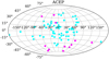 |
Fig. 1. Position on the sky in Galactic coordinates for the nine targets observed in this work (magenta filled circles in the southern hemisphere). The three complementary stars taken from the literature are also shown (magenta filled circles in the northern hemisphere). For comparison, light blue dots display the position of all the ACEPs in the Gaia DR3 catalogue. |
Basic data for the program stars and for the objects taken from the literature.
To further assess the classification as ACEPs of the 12 stars considered here, we report in Fig. A.1 their light curves in the Gaia bands. All the data were taken from DR3, with the exceptions of stars DR2 6498717390695909376 and DR2 2648605764784426624, which are only present in DR2 (see Ripepi et al. 2023, for explanations). The shapes of the light curves vary as the period increases from about one to about 2.25 days. In particular, EK Del, BF Ser and V716 Oph show asymmetric light curves with bumps and humps that are typical of ACEPs of the corresponding periods.
Figure 2 shows the period–Wesenheit (PW; The Wesenheit magnitudes are reddening-free by construction according to Madore 1982) relation in the Gaia bands (defined as G − 1.90 × (GBP − GRP), see Ripepi et al. 2019) for the 12 ACEPs analysed in this work in comparison with the ACEPs from the LMC. For the Galactic ACEPs, we obtained the photometry from Gaia Data Release 3 (Gaia Collaboration 2023; Ripepi et al. 2023), while the absolute Wesenheit magnitudes were calculated by inverting the Gaia parallaxes after correcting for the zero-point offset according to Lindegren et al. (2021; we are aware of the incorrectness of this procedure for parallaxes with relative error larger than about 10–15%, indeed the figure is only for illustrative purposes). Similarly, for the LMC, the photometry is from Gaia DR3, while absolute Wesenheit magnitudes have been derived by adopting a distance modulus of 18.477 ± 0.026 mag (Pietrzyński et al. 2019). The PW of the MW ACEPs we investigated are compatible with the expected position as traced by the well-known LMC objects, thus confirming the correctness of the classification. The only ACEP_1O star, namely HE 2324−1255, is an exception in the sense that its position in Fig. 2 agrees better with F-mode pulsators than with 1O-mode pulsators. However, the analysis of the light curves shown in Fig. A.1 leaves little doubt about its classification as an overtone pulsator.
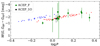 |
Fig. 2. Period–Wesenheit relation in the Gaia bands for the 11 ACEP_Fs (filled green circles) and one ACEP_1O (filled black circle, log P shifted by −0.01 to avoid overlap with F pulsators) in comparison with analoguous data for the LMC (red and blue dots represent ACEP_Fs and ACEP_1Os, respectively). To obtain the absolute Wesenheit magnitude for the LMC stars, we adopted the distance modulus by Pietrzyński et al. (2019). |
2.2. Observations and data reduction
The spectroscopic observations analysed here have been acquired with the European Southern Observatory (ESO) Ultraviolet and Visual Echelle Spectrograph (UVES)1 instrument, which is operated at the Unit Telescope 2 of Very Large Telescope (VLT), placed at Paranal (Chile). The data were obtained on 12–20 December 2020 in the context of proposal P106.2129.001, which was mostly devoted to observing a large sample of classical Cepheids that was published in Trentin et al. (2023). We adopted the red arm and grism CD 3, which has a central wavelength at 5800 Å and covers the wavelength interval 4760–6840 Å. We choose the 1 arcsec slit, which gives a dispersion of R ∼ 47 000. Because the instrumental setup was identical, we refer to Trentin et al. (2023) for full details of the data reduction steps that led to the production of the fully calibrated normalised spectra.
Figure A.1 shows the phases at which each star was observed. For the literature stars, the phases were taken from the source papers. BF Ser and V716 Oph were repeatedly observed at different phases. Only one phase is shown in the figure for homogeneity. The majority of the targets were observed in the quiescent descending branch. For a few stars, namely HE 0114−5929, DF Hyi, and SHM2017 J000.07389−10.22146, the observations instead fell on the fast-rising branch or at maximum light. Even though it is preferable to avoid these phases of the pulsation cycle, we do not expect that our abundance analysis is significantly affected (see e.g., Sect. 7 in For et al. 2011, for a discussion about this point in the context of RR Lyrae pulsators).
2.3. Atmospheric parameters
The chemical analysis was performed in essentially the same way as in Trentin et al. (2023). We briefly recall the main steps of the procedure. First, we estimated the atmospheric parameters, namely the effective temperature (Teff), surface gravity (log g), microturbulent velocity (ξ), and the line broadening parameter (vbr), that is, the combined effects of macroturbulence and rotational velocity.
Because the metallicity of these stars is low, the number of measurable spectral lines of Fe I in their spectrum is extremely limited. For this reason, in order to determine the atmospheric parameters necessary for chemical analysis, we had to proceed in two ways, depending on the number of detected iron lines.
For the stars for which a sufficient number of spectral lines could be measured, we applied the method of excitation equilibrium. This method ensures that there is no residual correlation between the iron abundance and the excitation potential of the neutral iron lines (see e.g., Mucciarelli & Bonifacio 2020). We estimated the microturbulence by requiring that the slope of [Fe/H] as a function of equivalent widths (EWs) is zero. To achieve this, we initially measured the equivalent widths of a sample of Fe I lines using a semi-automatic custom routine in IDL2. The conversion of EWs into abundance was performed using the WIDTH9 code (Kurucz & Avrett 1981) applied to the corresponding atmospheric model calculated using ATLAS9 (Kurucz 1993). In this calculation, we did not consider the influence of log g because neutral iron lines are insensitive to it. Next, we estimated the surface gravities iteratively by imposing the ionisation equilibrium between Fe I and Fe II.
The sample of Fe I and Fe II lines was extracted from the line list published by Romaniello et al. (2008).
For the remaining objects (HE 0114−5929 and SHM2017 J000.07389−10.22146), we estimated the temperature by fitting the Hβ profile. In practice, we minimised the difference between the observed and synthetic spectra using the χ2 as a goodness-of-fit parameter. The synthetic profile was generated in three steps, as described in the next section. It is known from the literature that the core of the Balmer lines is not reproduced by 1D-LTE models, for which 3D non-LTE models would be necessary. The global effects of non-LTE on Balmer lines were extensively studied by Mashonkina et al. (2008) and Amarsi et al. (2018). Both studies concluded that neglecting non-LTE effects in metal-poor stars leads to an underestimate of the effective temperature by approximately 150 K, which we took into account in the total error estimation. We determined the projected rotational velocities (vbr) of our targets by matching the synthetic line profiles to the Mg I triplet at λλ 5167-5183 Å, which is particularly useful for this purpose.
To compute the gravity for these stars, we modelled the lines of the Mg I triplet at λλ 5167, 5172, and 5183 Å, which are very sensitive to log g variations. First, we derived the magnesium abundance through the narrow Mg I lines at λ 5528 Å (not sensitive to log g), and then we fitted the triplet lines by fine-tuning the log g value. The microturbulence velocities for these stars were estimated using the calibration ξ = ξ(Teff, log g) published by Allende Prieto et al. (2004).
The estimated atmospheric parameters are summarised in Table 2.
Atmospheric parameters for the program stars.
2.4. Chemical abundances
Following the same procedure as adopted in Trentin et al. (2023), we chose the spectral synthesis approach to overcome problems due to the spectral line blending caused by line broadening. The synthetic spectra were generated in three steps: (i) LTE atmosphere models were computed using the ATLAS9 code (Kurucz 1993), using the stellar parameters in Table 2; (ii) stellar spectra were synthesised by using SYNTHE (Kurucz & Avrett 1981); and (iii) finally, the synthetic spectra were convolved for instrumental and line broadening.
The detected spectral lines allowed us to estimate the abundances for a total of 13 different chemical elements. For all targets, we performed the following analysis: We divided the observed spectra into intervals of 25 Å or 50 Å and derived the abundances in each interval by performing a χ2 minimisation of the differences between the observed and synthetic spectra. The minimisation algorithm was written in IDL language, using the amoeba routine.
We considered several sources of uncertainties in the abundance: δTeff, δlog g, and δξ. According to our simulations, these errors contribute ≈±0.1 dex to the total error budget. The total errors were evaluated by summing this value in quadrature to the standard deviations obtained from the average abundances.
The adopted lists of spectral lines and atomic parameters are taken from Castelli & Hubrig (2004), who updated the original parameters of Kurucz (1995). When necessary, we also checked the NIST database (Ralchenko & Reader 2019).
In the atmospheres of giant stars, departures from LTE calculations might be non-negligible. Recently, Amarsi et al. (2020) explored a wide range of non-LTE corrections for a number of chemical elements. For each of them, they also computed the difference between non-LTE and LTE abundances versus metallicities for dwarf and giant stars. We used their grids in order to evaluate the impact of non-LTE corrections on our results. In particular, because of the low metallicity of our targets, we neglected corrections for carbon, magnesium, silicon, calcium, and barium, while we applied a correction of 0.1 dex to our LTE sodium abundance.
A sample of the target star spectra is shown in Fig. 3. The final abundances are listed in Tables 3 and B.1 (where the abundances are expressed as [X/Fe] instead of [X/H]).
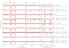 |
Fig. 3. Excerpt from our UVES spectra for the nine ACEPs. The black and red lines show the data and the best-fitting synthetic spectra, respectively. Some lines are labelled in the figure, as is the iron abundance. In the right panel, we show the fit of the Na I doublet at 5889–5895 Å. It is possible to note the interstellar sodium lines in four out of nine stars, for which we accurately fit only the line profile of the stellar sodium. |
Stellar abundances.
3. Results
To infer clues about the origin of the ACEPs, we compared their chemical abundances with those of stellar systems that might resemble the place of origin of the ACEPs, namely, the MW field, GGCs, dSph and UFDs. For the MW, we adopted the large sample of stars published in DR3 of the GALactic Archaeology with HERMES (GALAH) survey (Buder et al. 2021), selecting only stars with high-quality results (flag = 0 for each element) and with Galactic latitude b > |15| deg to avoid disk stars that might add confusion. For the GGCs, we adopted the results by Carretta et al. (2009a), while for the dwarf satellites of the MW, we used the vast and updated database SAGA (Stellar Abundances for Galactic Archaeology Database; Suda et al. 2008, 2017).
We divided the chemical species into two groups: (i) light and α-elements including Na (carbon is not discussed because we measured it only in four stars), Mg, Si, Ca, and Ti, and (ii) iron group (including also Sc, which is intermediate between α and iron) Cr and Ni and neutron-capture elements, Y and La.
To discuss the properties of the investigated ACEPs, we compare in Figs. 4 and 5 their abundances with those of the MW and GGC (when available). In a similar way, Figs. 6, 7; Figs. 8, 9, and Figs. 10, 11 show the comparison between the ACEP abundances and those of dSphs hosting an extended intermediate-old dSphs with a purely old stellar population and the abundances of UFDs, respectively.
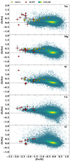 |
Fig. 4. Abundances of sodium, magnesium, silicon, calcium, and titanium for the ACEPs (solid red points with error bars) in comparison with GGCs (yellow stars) and the GALAH MW data. |
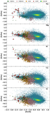 |
Fig. 6. Same as in Fig. 4, but for the comparison with three dSph hosting an extended intermediate-age population, namely Carina, Fornax and Leo I (see labels). |
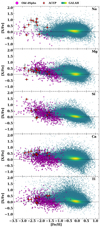 |
Fig. 8. Same as in Fig. 4, but for the comparison with several dSph hosting a purely old population. Becaus of the high number of galaxies, we display all the data with the same colour for clarity (magenta). |
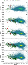 |
Fig. 10. Same as in Fig. 4, but for the comparison with several UFDs. Because of the high number of galaxies, we display all the data with the same colour for clarity (green). |
In the following, we discuss each element separately.
Sodium. In 9 of 11 ACEPs (EK Del has no Na measurement), we find a significant overabundance of sodium compared to all the comparison samples: average halo abundances (only a few GALAH stars with similar overabundances), Local Group dwarfs, and GGCs (average values). For the GGCs, we compared ACEPs Na abundances with those of individual cluster stars. This is reported in the histogram of Fig. 12, where we show the Na distribution of 1312 stars in 15 GGCs (data from Carretta et al. 2009b) in comparison with the 11 ACEPs with Na measurement. Several ACEPs have Na abundances in the region of the most extreme second-generation GGC stars or beyond. In particular, only about 4% of GGC stars have [Na/Fe] > 0.7 dex, while more than half of our sample shows values beyond this threshold. The two stars showing a small underabundance of Na are BF Ser and SHM2017 J000.07389−10.22146; V716 Oph has [Na/Fe] ∼ 0.35 dex, while all the other ACEPs have [Na/Fe] > 0.5 dex. In particular, HE 0114−5929, DF Hyi, and CRTS J003041.3−441620 show values of [Na/Fe] higher than 1 dex. We try to explain this significant feature in the following section.
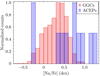 |
Fig. 12. Histogram of individual [Na/Fe] abundances for stars belonging to 15 GGCs (red) and the investigated ACEPs (blue). The GGCs data are from Carretta et al. (2009b). |
Magnesium. Similar to other α elements that we can measure (Ca, Si, and Ti), Mg is expected to be enhanced at low iron abundance values, but in a different way than the other three elements because it is produced during the hydrostatic He burning in massive stars. It is therefore less directly connected to the SN II explosion conditions (e.g., Tolstoy et al. 2009). Nevertheless, Fig. 4 shows a Mg enhancement for all the stars, with the significant exception of SHM2017 J000.07389−10.22146, which has [Mg/Fe] ∼ −0.4 dex, and EK Del, which has [Mg/Fe] ∼ 0 dex. In general, the location of the ACEPs in the [Mg/Fe] versus [Fe/H] diagram agrees very well with those of the Galactic halo stars and GGCs, and also with those of the dwarf satellites of the MW.
Silicon and titanium. We discuss these two α elements together because they show similar features. For both elements, we were unable to obtain a measure in DR2 6498717390695909376 and HE 0114−5929. Silicon is also absent for DR2 2976160827140900096 and BF Ser, while Ti is not measurable in SHM2017 J000.07389−10.22146. In the stars for which we have a measurement, Si and Ti are enhanced, as expected, but with three notable exceptions: the ACEPs HE 2324-1255, CRTS J003041.3−441620, and DF Hyi all show slightly negative values of both [Si/Fe] and [Ti/Fe] abundances, in contrast with the remaining five and six stars (in Si and Ti, respectively). The comparison with the MW field and GGCs (only Si) only agrees well with stars showing Si/Ti enhancement (see Fig. 4). The agreement with MW satellites is good only for the ACEPs with [Fe/H] < −2.2 dex, especially for the UFDs. The position of the three ACEPs with low [Si/Fe] and [Ti/Fe] values seems to be more consistent with the dwarfs possessing a purely old population, such as Draco or Ursa Minor, but both these galaxies show a wide range of Si and Ti abundances at fixed iron.
Calcium. Figure 4 shows that the calcium abundance of all the ACEPs considered here (except for SHM2017 J000.07389−10.22146 for which we were unable to measure this element) is enhanced and is in the range 0.3 < [Ca/Fe] < 0.75 dex, as expected for this pure α element. The agrement with the Galactic halo is generally very good, suggesting that both the ACEPs and the metal-poor halo stars were born at early times from material highly enriched by SN II ejecta (SN IIs produce large amounts of α elements in contrast with SN Ia which mostly provide iron, see e.g., Tolstoy et al. 2009). The comparison with all the MW satellites shows that at a fixed iron abundance, the ACEP [Ca/Fe] values are systematically higher, especially in the purely old dSphs and UFDs (Figs. 8 and 10).
Scandium. We have measures of Sc for seven stars, that is, no data for DR2 6498717390695909376, HE 0114−5929, SHM2017 J000.07389−10.22146, and EK Del. Figure 5 shows that the [Sc/Fe] value is negative for four stars, namely DR2 2976160827140900096, HE 2324−1255, CRTSJ003041.3−441620, and DF Hyi. Notably, the last three are the same stars for which the [Si/Fe] and [Ti/Fe] values were lower than for the other ACEPs. This underabundance of Sc for more than 50% of our stars is surprising because scandium is expected to be mainly produced during core-collapse SN events, with a small contribution from AGB stars (Kobayashi et al. 2020). There are virtually no stars in the GALAH sample with a negative value of [Sc/Fe] in the relevant [Fe/H] interval. The same applies to the dSphs with an extended intermediate-age population, while some negative [Sc/Fe] values can be found among the purely old dSphs a UFDs. In any case, the similarity of behaviour of the Si, Sc, and Ti for the three stars mentioned before might indicate a common origin of these three objects, even if they lie in very different regions of the Galactic halo.
Chromium. We measured Cr in all the stars except for SHM2017 J000.07389−10.22146. Chromium is an iron-peak element and is produced both in core-collapse and thermonuclear SNe. The measures for the ACEPs show values of [Cr/Fe] around zero within the errors, in fair agreement with the MW halo up to [Fe/H] ∼ −2.0 dex. Beyond this value, there are only a few measures. Compared with the dSph and UFD data, our Cr abundances appear systematically higher.
Nickel. We only have nickel measurements for five stars. All the measures are overabundant compared to iron, except for DR2 2648605764784426624, which has [Ni/Fe] ∼ 0 dex. The bulk of the Galactic data shows negative values of [Ni/Fe] at the [Fe/H] value of interest, even if there are scattered stars with positive values. The dSphs show a dispersion of values for [Ni/Fe], but with a tendency towards negative values in the relevant metallicity range.
Yttrium. Yttrium is a neutron-capture element that is mainly formed through s-process in AGB stars at solar metallicities, while at low metallicities, a contribution from the r-process is required to explain its abundance (Kobayashi et al. 2020). We have measures of yttrium for seven stars, three and four stars showing positive and negative [Y/Fe] values, respectively (see Fig. 5). Two of the stars with negative [Y/Fe], namely DF Hyi and CRTS J003041.3−441620, are among the triad of objects with low values of Si, Ti, and Sc abundances (we do not have measures for the third star HE 2324−1255). Compared with the Galactic and dSphs/UFDs sample, the overall distribution of the seven ACEPs in the [Y/Fe] versus [Fe/H] agrees well, but in the MW satellites, the measures are scarce and rather scattered.
Barium. Barium is an almost pure s-process element, but its high value at low [Fe/H] requires r-process to be at work (Kobayashi et al. 2020). We have Ba abundances for eight stars, as shown in Fig. 5. These measures show a significant degree of dispersion, in agreement with the Galactic and dSph abundances. The ACEP HE 2324−1255 shows a significantly low value of [Ba/Fe] (this is one of the triads with low Si, Ti, Sc, and possibly Y), but stars with a similar abundance can be found among the dSphs.
4. Discussion
The abundance analysis presented here provides new insights into the long-standing debate on the origin of the ACEPs. In this section, we consider old and new hypotheses, forming a basis for future investigations in order to definitively answer the many still open questions.
4.1. ACEPs as metal-poor objects
All ACEPs we investigated are metal-poor with −2.87 ≤ [Fe/H] ≤ −1.54 dex. Although it is based on a restricted sample of ACEPs, this result directly empirically confirms the theoretical prediction that does not forecast the possible occurrence of ACEPs for values of [Fe/H] higher than ∼ − 1.5 dex (see e.g., Fiorentino et al. 2006; Monelli & Fiorentino 2022). A spectroscopic investigation of the ACEPs detected in the direction of the bulge may be a good test for this expectation. In this region, the intermediate-age and old stellar populations (from which the ACEP originate) can be (significantly) more metal-rich than [Fe/H] ∼ −1.5 dex (see the review by Kunder 2022, for the Red Clump and RR Lyrae stars).
4.2. Possible extragalactic origin for the ACEPs
The MW ACEP composition resulting from our analysis agrees well with that of a typical population II star belonging to the Galactic halo, with the partial exception of sodium. Figure 4 shows a number of Galactic stars with [Fe/H] < −1.5 dex and [Na/Fe] > +0.5 dex, that is, the range in which more than half of the ACEPs are placed. However, the percentage of these Galactic stars is lower than 10% of all the GALAH stars with [Fe/H] < −1.5 dex. Even though the statistics are poor, a difference in the sodium abundance between the ACEPs and the metal-poor population of the Galactic Halo therefore appears to be present. We return to this point in Sect. 4.5.
Overall, the α-elements, Mg and Ca, in particular, are overabundant compared to iron. This is a well-known feature of population II stars, which are thought to form from primordial gas mostly enriched with the yields of core-collapse supernovae. Similarly, the heavier elements generally agree with the population II Galactic sample. Three stars, however, HE 2324−1255, CRTS J003041.3−441620, and DF Hyi, show low [Si/Fe], but quite high [Mg/Fe] and [Ca/Fe], while SHM2017 J000.07389−10.22146 shows negative [Mg/Fe] (−0.42 dex), but quite a high silicon overabundance ([Si/Fe] = +1.45 dex). At odds with all the other ACEPs in our sample, SHM2017 J000.07389−10.22146 is also sodium depleted ([Na/Fe] = −0.27 dex). One possibility to explain these anomalous compositions is to hypothesise that they are the consequence of local pollution of the gas from which these stars were born. The scatter of the α-element abundances is generally small in halo stars. For instance, in most stars with [Fe/H] < −1.5 dex, the magnesium overabundance ([Mg/Fe]) ranges between +0.1 dex and +0.5 dex, with an average [Mg/Fe] ∼ 0.3 dex (see e.g., Sneden et al. 2008). However, for a few halo stars, significantly different [α/Fe] values were found (see e.g., Ryan et al. 1996; Ivans et al. 2003). This occurrence represents evidence of a certain degree of inhomogeneity in the early Galaxy.
On the other hand, the comparison of the MW ACEP composition with that of the stellar populations harboured in dSph and UFD galaxies reveals more differences than similarities. In addition to sodium, which is discussed below, the main differences are as follows: (i) Figs. 6, 8, and 10 show that the distribution of the [Ca/Fe] abundances in the MW satellite appears to be systematically lower than that of ACEPs, but it is not completely incompatible in the case of the old dSph and UFDs. (ii) Similar to Ca, Figs. 7, 9, and 11 show that chromium (and possibly nickel) in ACEPs is systematically more abundant than in the MW satellites.
The most noticeable difference is in the abundance of sodium. Figures 6, 8 and 10 show that the MW satellites do not have stars with high [Na/Fe] values at the metallicity of ACEPs. However, two objects, SHM2017 J000.07389−10.22146 and BF Ser, display negative [Na/Fe] values, while V716 Oph has [Na/Fe] ∼ 0.35 dex and is compatible with the abundances of old dSphs and UFDs. To investigate the possibility that these stars at least can originate from a merging of one of these objects, we display in the left panel of Fig. 13 the angular momentum in the z direction LZ versus the energy of the orbit for the investigated ACEPs in comparison with those of GGCs, which are in large part thought to have been accreated during ancient mergers (e.g., Massari et al. 2019; Kruijssen et al. 2020). The details concerning the calculation of these parameters are reported in Appendix C. The location of the three ACEPs with negative or mildly positive [Na/Fe] values is on the retrograde side of the plot (negative values of LZ). This feature can reveal an extragalactic origin. However, also DF Hyi and DR2 2648605764784426624, which show high values of [Na/Fe] that are not present in MW satellites, have retrograde motion. It is therefore difficult to draw firm conclusions about the extragalactic origin of the aforementioned three stars, also in light of the difference in calcium an chromium. An exception might be SHM2017 J000.07389−10.22146, which displays not only a strong retrograde motion, but also high energy, as is typical of dwarf galaxy satellites of the MW, as shown in the right panel of Fig. 13. When we also consider its other chemical anomalies, SHM2017 J000.07389−10.22146 is the most likely candidate in our sample of ACEPs to have an extragalactic origin.
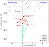 |
Fig. 13. Angular momentum in the z direction vs total energy of the orbit of the ACEP sample studied in this paper (filled red circles) in comparison with a sample of 166 GGCs (smaller filled light green circles) and of dwarf galaxies of the Local Group (smaller filled grey circles). To avoid confusion, the long identification names of some stars were abbreviated as follows: CRTS = CRTS J003041.3−441620; DR2_96 = DR2 2976160827140900096; HE_29 = HE 0114-5929; HE_55 = HE2324−1255; OGLE_006 = OGLE GAL-ACEP-006; SHM = SHM2017J000.07389−10.22146; DR2_24 = DR2 2648605764784426624; DR2_76 = DR2 6498717390695909376. |
In conclusion, a scenario in which the ACEPs found in our Galaxy were assembled in metal-poor extragalactic environments and were later on captured by the gravitational potential well of the Milky Way, appears disfavoured by the observed abundance pattern, with the notable exception of SHM2017 J000.07389−10.22146.
4.3. ACEPs as single stars
Based on their composition and kinematics, the MW ACEPs in our stellar sample appear to be typical Galactic halo stars. On the other hand, their luminosity, colour, and pulsational properties all indicate that the current mass of these core-He burning stars ranges between 1.3 and 2.5 M⊙, which corresponds to single-star ages between 1 and 6 Gyr. Intermediate-age stellar populations like this are commonly found in dwarf galaxies, but halo stars are definitely older. There are, indeed, multiple pieces of evidence confirming that star formation in the Galactic halo ceased no later than 10 Gyr ago (see e.g., Haywood et al. 2016, and references therein).
On the other hand, the chemical pattern discussed in previous sections causes us to exclude an extragalactic origin for the MW ACEPs. Therefore, it appears that these stars must be old, with ages of 10 Gyr or older, but their present-day mass should be higher than 1.2 M⊙. The only known scenarios explaining old and massive core-He burning stars are those involving binary systems that originally consisted of two low-mass companions whose evolutionary lifetime is comparable to or longer than the halo age (Renzini et al. 1977). According to these scenarios, after a sufficiently large portion of their single-star lifetime, the two components of the binary system interact through a mass transfer process (Roche-lobe overflow) and eventually a coalescence. Most likely, the binary interaction occurred when the two stars were both on the main sequence. In this case, a BS would form. Then, after the central-H exhaustion, the BS evolves, becomes a red giant, and later on, a core-He burning star. If the mass of this core-He burning star is in the range between 1.2 and 2.1 M⊙, it will become an ACEP pulsator. Alternatively, the binary interaction occurred after the primary evolved out of the main sequence when the star became a red giant star. In this case, the final outcome may be very different depending on the initial orbital parameters and on whether the mass transfer is conservative (total mass and total angular momentum are conserved). In any case, because the donor has an extended convective envelope, its radius increases as its mass is eroded. In addition, until the mass ratio M1/M2 > 1, the two components of the binary approach each other, and the mass transfer rate is in turn expected to be quite fast at the beginning. In these conditions, the amount of mass that the secondary star may actually accept is rather uncertain. Later on, when the mass ratio becomes lower than 1, the separation increases and the mass transfer rate becomes slower. In any case, the mass transfer should continue until the whole envelope of the giant star is lost or the RGB tip is reached. In practice, the masses of the two components and the separation after this mass transfer episode depend on a complex phenomenology. Then, if the final mass of the secondary exceeds 1.2 M⊙ and no further mass transfers occur, it may eventually become an ACEP. Renzini et al. (1977) found that a fairly wide range of initial separations exists for which this scenario may result in the formation of an ACEP on a timescale of about 10 Gyr. However, they assumed conservative mass transfer. In the two binary scenarios described above, main-sequence star merger or RGB mass transfer, the Galactic ACEPs would be descendants of BSs.
In summary, our data suggest that the Galactic ACEPs investigated in this paper probably originated in a binary star.
4.4. Stars that may synthesise sodium and the abundances that correlate with sodium enhancement
Sodium is produced by proton captures on 22Ne in the H-burning shell of RGB, AGB, and massive giant stars. When a deep mixing process sets on, additional 22Ne is moved down to the layers in which the H-burning takes place, while freshly synthesised 23Na is dredged up to the stellar surface. Extant nucleosynthesis models show that in order to obtain this sodium enhancement, temperatures as high as 20–30 MK should be attained by this external circulation (see next section). This is known to occur in massive AGB stars (M > 3 − 4 M⊙), in which the convective envelope penetrates inward down to the hottest layers of the H-burning shell. This process is called hot bottom burning (HBB). In massive stars (M > 20 − 25 M⊙), the required deep mixing may be activated in case of fast rotation (e.g., Decressin et al. 2007). In all other cases, such as in RGB stars, other instabilities might also induce mixing below the convective envelope, such as gravity waves generated at the convective border (Denissenkov & Tout 2003), magnetic buoyancy (Busso et al. 2007), or thermohaline circulation (Charbonnel & Zahn 2007). In all these cases, the Na enhancement is thought to be associated with a significant N enhancement, while O is thought to be depleted. Unfortunately, we do not have O and N lines in our spectra, but the search for these correlations/anti-correlations may be the goal of future investigations. Na can be also produced by neutron capture on 22Ne, followed by the β decay of the radioactive 23Ne. In a low-mass AGB star, a 13C pocket forms after each third dredge-up episode, and later on, neutrons are released by the 13C(α, n)16O reaction (Straniero et al. 2006; Cristallo et al. 2009). In this environment, the bulk production of the s-process main component occurs in nature. In this case, the third dredge-up also causes the atmospheric sodium enrichment, which is thought to be associated with strong enhancements of both C and s-process elements. For a few ACEPs, we observed Y and Ba, and these measurements seem to exclude that the Na enhancement is a consequence of a low-mass AGB pollution. The measured abundances of these heavy elements are those typically found in halo stars, in which they originate from the r-process, rather than from the s-process (Sneden et al. 2008).
We finally note that both HBB, active in massive AGB stars, and rotation-induced mixing, eventually active in fast-rotating massive stars, are also thought to produce a substantial He enhancement. A certain He enhancement is also expected in case of activation of a deep-mixing process in RGB and low-mass AGB stars. The He abundance cannot be easily measured in ACEP stars. However, according to Kovtyukh et al. (2018), a helium overabundance is thought to affect the light curves of these pulsators. Theory predicts that for a variety of pulsating variables, higher He implies smaller amplitude and more sinusoidal (i.e. less asymmetric) light curves (Marconi et al. 2016). Therefore, we searched for a correlation between the abundance of Na and the amplitude in G mag of the MW ACEPs. This test is shown in Fig. 14. The expected correlation is clearly recognised (correlation coefficient = −0.79), especially when we do not consider the two ACEP_F CRTS J003041.3−441620 and DF Hyi, which show low Si, Ti, and Sc abundances (the third ACEP, HE 2324−1255 is a 1O pulsator and has a low amplitude for this reason), thus possibly showing an additional anomaly compared with the other ACEPs. In summary, there is more than one channel to synthesise sodium in AGB or massive stars. In any case, an overabundance of Na is thought to be coupled with an overabundance of He. Pulsational arguments suggest that our stars show a correlation between the [Na/Fe] value and the He abundance.
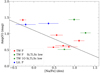 |
Fig. 14. Visual amplitude of the observed ACEPs as a function of the [Na/Fe] abundance. The solid line shows a linear regression to the data that does not include the three stars with low values of the [Si/Fe], [Ti/Fe] and [Sc/Fe] abundances (green symbols, see labels). In the labels, TW and Lit. indicate the nine stars that were studied spectroscopically in this paper and the three with spectroscopy from the literature, respectively. |
4.5. Origin of the [Na/Fe] overabundance
As already remarked, the most notable result of our analysis are the high [Na/Fe] values we found in 9 out of 11 stars in our sample for which the Na values were measurable. A high overabundance of sodium, associated with nitrogen, and possibly helium enhancements and oxygen depletion are typical of some GC stars. According to the most popular scenario, the Na overabundance is the result of self-pollution. The polluters would have been first-generation AGB stars or fast-rotating massive stars, while the second generation of stars, which formed from the gas lost by the polluters, are those showing the mentioned chemical peculiarities (see e.g., Gratton et al. 2012, and references therein). In contrast, the large majority of the field halo stars show scaled solar sodium. A possible Na–O anti-correlation was recently found in a sample of type II Cepheids (BL Her pulsators; Kovtyukh et al. 2018).
In the previous sections, we excluded an extragalactic origin for the MW ACEPs based on the observed chemical pattern. When they are field stars of the MW halo, we need to explain the Na overabundance. There are various possibilities:
The MW ACEP progenitors were Na-rich GC stars. Several problems affect this hypothesis. First of all, ACEPs are very rare in GCs, there are only two confirmed objects (see Sect. 1). In addition, as previously discussed, MW ACEPs are more likely the descendants of interactive binaries, and the estimated ACEP masses are substantially higher than that of the other cluster stars. They are therefore expected to be more centrally concentrated in a GC and more gravitationally bound. Finally, the number of second-generation stars is comparable to those of the first generation. Therefore, we should observe a comparable number of ACEPs with and without sodium enhancement, which contradicts our results.
In a recent paper, Belokurov & Kravtsov (2023) found that about 4% of the Galactic stars with [Fe/H] < −1.5 dex show high [N/O] abundances, which would also imply high [Na/Fe] values. According to the authors, these objects originated from second-generation stars produced at early times in now completely disrupted GCs. These stars clearly are the perfect progenitors for the ACEPs we analysed, but statistical considerations suggest that they can only account for one object maximum, as we observe high [Na/Fe] in 9 of the 11 ACEPs. In conclusion, the hypothesis that MW ACEPs were born in GCs appears quite unlikely.
Na enrichment as a consequence of a mass transfer from a massive AGB or a fast-rotating massive star companion in a binary system. As already mentioned, the wind of massive AGB stars experiencing HBB or that of fast-rotating massive stars might in principle be the source of the required Na enrichment. However, the involved timescales are too short. To transfer a sufficient amount of Na, the donor must be a rather massive object (≥4 M⊙). In the most favourable case, the accretion occurred just ∼0.1 Gyr since the binary formation. Even considering a final accretor mass as low as 1.2 M⊙ (the minimum mass for an ACEP), the total lifetime is in any case no more than 6 Gyr, which is definitely shorter than the halo age. In addition, when a massive AGB experiences Roche-lobe overflow, a common envelope likely takes place so that most of the envelope mass would be lost. This inconvenience would be avoided in case of wind accretion.
Na enrichment as a result of an intrinsic nucleosynthesis. Current stellar models show that Na is produced in the H-burning shell of RGB stars at a temperature between 20 and 30 MK. The temperature at the base of the convective envelope is much lower, so that in order for sodium to be enhanced at the stellar surface, a further deep-mixing process penetrating the external tail of the H-burning shell is needed. Fast rotation may provide the engine for this process. If MW ACEPs originate from low-mass interacting binaries, main-sequence stars mergers, or RGB mass transfer (see previous section), an efficient angular momentum transfer would cause a significant gain in the rotational speed of the progenitor. After this foundation event, a fast-rotating BS would form that later evolves into a fast-rotating red giant. Then, meridional circulations or other rotational-induced instabilities, such as those due to shear between a fast-rotating envelope and a slow-rotating core, may activate a mixing process in the region between the inner border of the convective envelope and the H-burning shell. To quantify the resulting sodium overabundance, we computed some test models of RGB stars with masses of 1.2 and 1.5 M⊙ and the typical composition of metal-poor halo stars, namely [Fe/H] = −2.1 dex, [α/Fe] = 0.4 dex, and initial He mass fraction Y = 0.25. These models were computed by means of FuNS, a stellar evolution code that is widely used to model stars of any mass and composition, with or without rotation, whose latest version is described in Straniero et al. (2019, 2020). In our models, a deep mixing below the convective envelope is switched on after the star attains the RGB bump luminosity. Before this point, the deep mixing is prevented by the sharp molecular-weight gradient that is left by the first dredge-up. The RGB bump occurs when the H-burning shell reaches this layer, and the μ-gradient is smoothed out. The resulting Na overabundance is illustrated in Fig. 15.
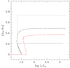 |
Fig. 15. Sodium overabundances in RGB stellar models undergoing a rotation-induced deep-mixing process. The black lines refer to 1.2 M⊙ models, and the red line plots a 1.5 M⊙ model. The solid, long-dashed, and dotted lines represent cases in which the deep-mixing attains a maximum temperature of Tmax = 19, 23, and 27 MK, respectively. |
Here, the deep-mixing process depends on two free parameters, namely the maximum temperature attained at the deepest mixed layer, and the average mixing velocity. The resulting sodium enhancement mainly depends on the former, while a variation of the latter has a weaker effect.
Indications in favour of this intrinsic nucleosynthesis scenario are provided by some evidence that a large fraction of BSs are fast-rotating stars with spin rates generally above 50 km s−1 and up to 150 km s−1 (e.g., Shara et al. 1997; Lovisi et al. 2010; Mucciarelli et al. 2014; Sills 2016). More interesting is the recent finding by Ferraro et al. (2023) that the frequency of fast-rotating BSs is higher in loose GCs, those where the rate of lost stars should be also higher.
To summarise, the binary origin may simultaneously explain the average ACEP composition, which is that typical of Galactic halo stars, the anomalous Na overabundances, their relatively high masses, and their long lifetime.
5. Conclusions
We presented the first high-resolution spectroscopic analysis for a sample of 9 ACEPs belonging to the Galactic halo. The analysis of these spectra allowed us to derive the abundances of 12 elements, C, Na, Mg, Si, Ca, Sc, Ti, Cr, Fe, Ni, Y, and Ba. We complemented these data with literature abundances from high-resolution spectroscopy for an additional 3 ACEPs that were previously incorrectly classified as type II Cepheids, bringing the investigated objects to a total of 12. We studied the chemical properties of the ACEPs in comparison with Galactic field stars, GGCs, dSph, and UFD galaxy satellites of the MW. The main results of this work are listed below.
-
All the investigated ACEPs are metal poor, with [Fe/H] < −1.5 dex. This confirms the theoretical predictions asserting that a star can only enter the instability strip to become an ACEP when [Fe/H] is lower than about −1.5 dex.
-
The diagrams of the abundance ratios [X/Fe] versus [Fe/H] for the different elements show that at fixed [Fe/H], the position of the ACEPs is generally consistent with those of the Galactic halo field stars as measured by the GALAH survey, with the exception of the sodium abundance, which is overabundant in all the ACEPs but two. This is similar to second-generation stars in the GGCs. According to recent results, a fraction of the Galactic field halo stars can derive from stars like this, but based on statistical considerations, they cannot explain the sodium overabundance for 80% of the ACEPs we investigated.
-
The same comparison with dSphs and UFDs reveals more differences than similarities, not only for sodium, but also for other α elements, such as calcium and chromium. In general, a scenario in which the ACEPs found in our Galaxy were assembled in metal-poor extragalactic environments and were later on captured by the gravitational potential well of the Milky Way appears disfavoured by the observed abundance pattern, with the noticeable exception of star SHM2017 J000.07389−10.22146, which has a negative [Na/Fe] value, whose orbit shows strong retrograde motion, and the energy of which is comparable with that typical of dwarf galaxies satellite of the MW.
-
To explain the global characteristics of the investigated ACEPs and in particular, their supposed old age and peculiar chemical abundances, the most likely explanation is that they are binary stars.
-
We explored several possibilities to explain the anomalously high abundance of sodium in the ACEP atmospheres. At the moment, the best explanation is the evolution of low-mass stars in a binary system with either mass transfer or merging, which results in a rotational speed-up of the star due to the conservation of angular momentum, which in turn can trigger rotational mixing that is able to bring the products of internal nuclear burning to the surface. However, detailed modelling is needed to confirm this hypothesis.
The findings reported in this work must be corroborated by the observation of a larger sample of ACEPs by means of high-resolution spectroscopy. To this end, the advent of large spectroscopic surveys such as those foreseen with the WEAVE (WHT Enhanced Area Velocity Explorer)3 and 4MOST (4-m Multi-Object Spectroscopic Telescope)4 will certainly provide us with the statistics needed to draw more firm conclusions about the origin of the ACEP pulsators in our Galaxy.
Acknowledgments
We thank our anonymous Referee for their helpful comments which helped us to improve the paper. V.R. wishes to thank Zdenek Prudil for his help with the use of the Galpy package. This work was partially supported by the INAF-GTO program 2023: “C-MetaLL – Cepheid metallicity in the Leavitt law” (P.I. V. Ripepi). Part of this work was supported by the German Deutsche Forschungsgemeinschaft, DFG project number Ts 17/2–1. This research has made use of the SIMBAD database, operated at CDS, Strasbourg, France. This work has made use of data from the European Space Agency (ESA) mission Gaia (https://www.cosmos.esa.int/gaia), processed by the Gaia Data Processing and Analysis Consortium (DPAC, https://www.cosmos.esa.int/web/gaia/dpac/consortium). Funding for the DPAC has been provided by national institutions, in particular, the institutions participating in the Gaia Multilateral Agreement. M.M. acknowledges financial support from the Spanish Ministry of Science and Innovation (MICINN) through the Spanish State Research Agency, under Severo Ochoa Programe 2020–2023 (CEX2019-000920-S), and from the Agencia Estatal de Investigación del Ministerio de Ciencia e Innovación (MCINN/AEI) under the grant “RR Lyrae stars, a lighthouse to distant galaxies and early galaxy evolution” and the European Regional Development Fund (ERDF) with reference PID2021-127042OB-I00.
References
- Allende Prieto, C., Barklem, P. S., Lambert, D. L., & Cunha, K. 2004, A&A, 420, 183 [NASA ADS] [CrossRef] [EDP Sciences] [Google Scholar]
- Amarsi, A. M., Nordlander, T., Barklem, P. S., et al. 2018, A&A, 615, A139 [NASA ADS] [CrossRef] [EDP Sciences] [Google Scholar]
- Amarsi, A. M., Lind, K., Osorio, Y., et al. 2020, A&A, 642, A62 [EDP Sciences] [Google Scholar]
- Baade, W., & Swope, H. H. 1961, AJ, 66, 300 [NASA ADS] [CrossRef] [Google Scholar]
- Bailer-Jones, C. A. L., Rybizki, J., Fouesneau, M., Demleitner, M., & Andrae, R. 2021, AJ, 161, 147 [Google Scholar]
- Baldacci, L., Rizzi, L., Clementini, G., & Held, E. V. 2005, A&A, 431, 1189 [NASA ADS] [CrossRef] [EDP Sciences] [Google Scholar]
- Baumgardt, H., & Vasiliev, E. 2021, MNRAS, 505, 5957 [NASA ADS] [CrossRef] [Google Scholar]
- Belokurov, V., & Kravtsov, A. 2023, MNRAS, 525, 4456 [NASA ADS] [CrossRef] [Google Scholar]
- Bernard, E. J., Monelli, M., Gallart, C., et al. 2009, ApJ, 699, 1742 [NASA ADS] [CrossRef] [Google Scholar]
- Bernard, E. J., Monelli, M., Gallart, C., et al. 2013, MNRAS, 432, 3047 [Google Scholar]
- Bersier, D., & Wood, P. R. 2002, AJ, 123, 840 [Google Scholar]
- Bono, G., Caputo, F., Santolamazza, P., Cassisi, S., & Piersimoni, A. 1997, AJ, 113, 2209 [NASA ADS] [CrossRef] [Google Scholar]
- Bovy, J. 2015, ApJS, 216, 29 [NASA ADS] [CrossRef] [Google Scholar]
- Buder, S., Sharma, S., Kos, J., et al. 2021, MNRAS, 506, 150 [NASA ADS] [CrossRef] [Google Scholar]
- Busso, M., Wasserburg, G. J., Nollett, K. M., & Calandra, A. 2007, ApJ, 671, 802 [NASA ADS] [CrossRef] [Google Scholar]
- Caputo, F. 1998, A&ARv, 9, 33 [NASA ADS] [CrossRef] [Google Scholar]
- Caputo, F., Castellani, V., Degl’Innocenti, S., Fiorentino, G., & Marconi, M. 2004, A&A, 424, 927 [NASA ADS] [CrossRef] [EDP Sciences] [Google Scholar]
- Carretta, E., Bragaglia, A., Gratton, R., & Lucatello, S. 2009a, A&A, 505, 139 [NASA ADS] [CrossRef] [EDP Sciences] [Google Scholar]
- Carretta, E., Bragaglia, A., Gratton, R. G., et al. 2009b, A&A, 505, 117 [NASA ADS] [CrossRef] [EDP Sciences] [Google Scholar]
- Castellani, V., & degl’Innocenti, S. 1995, A&A, 298, 827 [NASA ADS] [Google Scholar]
- Castelli, F., & Hubrig, S. 2004, A&A, 425, 263 [NASA ADS] [CrossRef] [EDP Sciences] [Google Scholar]
- Charbonnel, C., & Zahn, J. P. 2007, A&A, 467, L15 [NASA ADS] [CrossRef] [EDP Sciences] [Google Scholar]
- Clementini, G., Cignoni, M., Contreras Ramos, R., et al. 2012, ApJ, 756, 108 [NASA ADS] [CrossRef] [Google Scholar]
- Clementini, G., Ripepi, V., Leccia, S., et al. 2016, A&A, 595, A133 [NASA ADS] [CrossRef] [EDP Sciences] [Google Scholar]
- Clementini, G., Ripepi, V., Molinaro, R., et al. 2019, A&A, 622, A60 [NASA ADS] [CrossRef] [EDP Sciences] [Google Scholar]
- Coppola, G., Marconi, M., Stetson, P. B., et al. 2015, ApJ, 814, 71 [Google Scholar]
- Cristallo, S., Straniero, O., Gallino, R., et al. 2009, ApJ, 696, 797 [NASA ADS] [CrossRef] [Google Scholar]
- Decressin, T., Meynet, G., Charbonnel, C., Prantzos, N., & Ekström, S. 2007, A&A, 464, 1029 [NASA ADS] [CrossRef] [EDP Sciences] [Google Scholar]
- Denissenkov, P. A., & Tout, C. A. 2003, MNRAS, 340, 722 [NASA ADS] [CrossRef] [Google Scholar]
- Dolphin, A. E., Saha, A., Claver, J., et al. 2002, AJ, 123, 3154 [Google Scholar]
- Drake, A. J., Graham, M. J., Djorgovski, S. G., et al. 2014, ApJS, 213, 9 [Google Scholar]
- Ferraro, F. R., Mucciarelli, A., Lanzoni, B., et al. 2023, Nat. Commun., 14, 2584 [NASA ADS] [CrossRef] [Google Scholar]
- Fiorentino, G., & Monelli, M. 2012, A&A, 540, A102 [NASA ADS] [CrossRef] [EDP Sciences] [Google Scholar]
- Fiorentino, G., Limongi, M., Caputo, F., & Marconi, M. 2006, A&A, 460, 155 [NASA ADS] [CrossRef] [EDP Sciences] [Google Scholar]
- For, B.-Q., Sneden, C., & Preston, G. W. 2011, ApJS, 197, 29 [Google Scholar]
- Gaia Collaboration (Prusti, T., et al.) 2016, A&A, 595, A1 [NASA ADS] [CrossRef] [EDP Sciences] [Google Scholar]
- Gaia Collaboration (Brown, A. G. A., et al.) 2018, A&A, 616, A1 [NASA ADS] [CrossRef] [EDP Sciences] [Google Scholar]
- Gaia Collaboration (Brown, A. G. A., et al.) 2021, A&A, 649, A1 [NASA ADS] [CrossRef] [EDP Sciences] [Google Scholar]
- Gaia Collaboration (Vallenari, A., et al.) 2023, A&A, 674, A1 [NASA ADS] [CrossRef] [EDP Sciences] [Google Scholar]
- Gallart, C., Aparicio, A., Freedman, W. L., et al. 2004, AJ, 127, 1486 [NASA ADS] [CrossRef] [Google Scholar]
- Gatto, M., Ripepi, V., Bellazzini, M., et al. 2022, A&A, 664, L12 [NASA ADS] [CrossRef] [EDP Sciences] [Google Scholar]
- Gautschy, A., & Saio, H. 2017, MNRAS, 468, 4419 [NASA ADS] [CrossRef] [Google Scholar]
- Gratton, R. G., Carretta, E., & Bragaglia, A. 2012, A&ARv, 20, 50 [CrossRef] [Google Scholar]
- Green, G. 2018, J. Open Source Softw., 3, 695 [NASA ADS] [CrossRef] [Google Scholar]
- Haywood, M., Lehnert, M. D., Di Matteo, P., et al. 2016, A&A, 589, A66 [NASA ADS] [CrossRef] [EDP Sciences] [Google Scholar]
- Hoessel, J. G., Saha, A., Krist, J., & Danielson, G. E. 1994, AJ, 108, 645 [NASA ADS] [CrossRef] [Google Scholar]
- Ivans, I. I., Sneden, C., James, C. R., et al. 2003, ApJ, 592, 906 [NASA ADS] [CrossRef] [Google Scholar]
- Jurkovic, M. I. 2018, Serb. Astron. J., 197, 13 [NASA ADS] [Google Scholar]
- Kobayashi, C., Karakas, A. I., & Lugaro, M. 2020, ApJ, 900, 179 [Google Scholar]
- Kovtyukh, V., Yegorova, I., Andrievsky, S., et al. 2018, MNRAS, 477, 2276 [NASA ADS] [CrossRef] [Google Scholar]
- Kruijssen, J. M. D., Pfeffer, J. L., Chevance, M., et al. 2020, MNRAS, 498, 2472 [NASA ADS] [CrossRef] [Google Scholar]
- Kuehn, C., Kinemuchi, K., Ripepi, V., et al. 2008, ApJ, 674, L81 [NASA ADS] [CrossRef] [Google Scholar]
- Kunder, A. M. 2022, Universe, 8, 206 [NASA ADS] [CrossRef] [Google Scholar]
- Kurucz, R. L. 1993, IAU Colloq. (Cambridge: Cambridge University Press), 138, 87 [NASA ADS] [Google Scholar]
- Kurucz, R. 1995, Atomic Line List (Cambridge: Smithsonian Astrophysical Observatory) [Google Scholar]
- Kurucz, R. L., & Avrett, E. H. 1981, SAO Special Report, 391 [Google Scholar]
- Lindegren, L., Bastian, U., Biermann, M., et al. 2021, A&A, 649, A4 [EDP Sciences] [Google Scholar]
- Lovisi, L., Mucciarelli, A., Ferraro, F. R., et al. 2010, ApJ, 719, L121 [NASA ADS] [CrossRef] [Google Scholar]
- Luck, R. E., & Lambert, D. L. 2011, AJ, 142, 136 [Google Scholar]
- Madore, B. F. 1982, ApJ, 253, 575 [NASA ADS] [CrossRef] [Google Scholar]
- Marconi, M., Fiorentino, G., & Caputo, F. 2004, A&A, 417, 1101 [NASA ADS] [CrossRef] [EDP Sciences] [Google Scholar]
- Marconi, M., Coppola, G., Bono, G., Braga, V., & Pietrinferni, A. 2016, Commmun. Konkoly Obs. Hungary, 105, 125 [NASA ADS] [Google Scholar]
- Martínez-Vázquez, C. E., Monelli, M., Cassisi, S., et al. 2021, MNRAS, 508, 1064 [CrossRef] [Google Scholar]
- Mashonkina, L., Zhao, G., Gehren, T., et al. 2008, A&A, 478, 529 [NASA ADS] [CrossRef] [EDP Sciences] [Google Scholar]
- Massari, D., Koppelman, H. H., & Helmi, A. 2019, A&A, 630, L4 [NASA ADS] [CrossRef] [EDP Sciences] [Google Scholar]
- Mateo, M., Fischer, P., & Krzeminski, W. 1995, AJ, 110, 2166 [NASA ADS] [CrossRef] [Google Scholar]
- McConnachie, A. W., & Venn, K. A. 2020, Res. Am. Astron. Soc., 4, 229 [Google Scholar]
- McCrea, W. H. 1964, MNRAS, 128, 147 [Google Scholar]
- McMillan, P. J. 2017, MNRAS, 465, 76 [NASA ADS] [CrossRef] [Google Scholar]
- Monelli, M., & Fiorentino, G. 2022, Universe, 8, 191 [NASA ADS] [CrossRef] [Google Scholar]
- Monelli, M., Bernard, E. J., Gallart, C., et al. 2012, MNRAS, 422, 89 [NASA ADS] [CrossRef] [Google Scholar]
- Mucciarelli, A., & Bonifacio, P. 2020, A&A, 640, A87 [NASA ADS] [CrossRef] [EDP Sciences] [Google Scholar]
- Mucciarelli, A., Lovisi, L., Ferraro, F. R., et al. 2014, ApJ, 797, 43 [NASA ADS] [CrossRef] [Google Scholar]
- Musella, I., Ripepi, V., Marconi, M., et al. 2012, ApJ, 756, 121 [NASA ADS] [CrossRef] [Google Scholar]
- Nemec, J. M., Wehlau, A., & Mendes de Oliveira, C. 1988, AJ, 96, 528 [Google Scholar]
- Ngeow, C.-C., Bhardwaj, A., Graham, M. J., et al. 2022, AJ, 164, 191 [NASA ADS] [CrossRef] [Google Scholar]
- Norris, J., & Zinn, R. 1975, ApJ, 202, 335 [NASA ADS] [CrossRef] [Google Scholar]
- Ordoñez, A. J., Yang, S.-C., & Sarajedini, A. 2014, ApJ, 786, 147 [CrossRef] [Google Scholar]
- Piatti, A. E. 2015, MNRAS, 451, 3219 [NASA ADS] [CrossRef] [Google Scholar]
- Pietrzyński, G., Graczyk, D., Gallenne, A., et al. 2019, Nature, 567, 200 [Google Scholar]
- Plachy, E., & Szabó, R. 2021, Front. Astron. Space Sci., 7, 81 [NASA ADS] [CrossRef] [Google Scholar]
- Ralchenko, A. K., & Reader, J. 2019, National Institute of Standards and Technology, Gaithersburg, MD, https://dx.doi.org/10.18434/T4W30F [Google Scholar]
- Renzini, A., Mengel, J. G., & Sweigart, A. V. 1977, A&A, 56, 369 [NASA ADS] [Google Scholar]
- Ripepi, V., Marconi, M., Moretti, M. I., et al. 2014, MNRAS, 437, 2307 [Google Scholar]
- Ripepi, V., Molinaro, R., Musella, I., et al. 2019, A&A, 625, A14 [NASA ADS] [CrossRef] [EDP Sciences] [Google Scholar]
- Ripepi, V., Clementini, G., Molinaro, R., et al. 2023, A&A, 674, A17 [NASA ADS] [CrossRef] [EDP Sciences] [Google Scholar]
- Romaniello, M., Primas, F., Mottini, M., et al. 2008, A&A, 488, 731 [NASA ADS] [CrossRef] [EDP Sciences] [Google Scholar]
- Ryan, S. G., Norris, J. E., & Beers, T. C. 1996, ApJ, 471, 254 [Google Scholar]
- Schlafly, E. F., & Finkbeiner, D. P. 2011, ApJ, 737, 103 [Google Scholar]
- Shara, M. M., Saffer, R. A., & Livio, M. 1997, ApJ, 489, L59 [NASA ADS] [CrossRef] [Google Scholar]
- Siegel, M. H., & Majewski, S. R. 2000, AJ, 120, 284 [Google Scholar]
- Sills, A. 2016, Mem. Soc. Astron. Ital., 87, 475 [Google Scholar]
- Sills, A., Karakas, A., & Lattanzio, J. 2009, ApJ, 692, 1411 [NASA ADS] [CrossRef] [Google Scholar]
- Smith, H. A., & Stryker, L. L. 1986, AJ, 92, 328 [NASA ADS] [CrossRef] [Google Scholar]
- Sneden, C., Cowan, J. J., & Gallino, R. 2008, ARA&A, 46, 241 [Google Scholar]
- Soszyński, I., Udalski, A., Szymański, M. K., et al. 2015, Acta Astron., 65, 233 [NASA ADS] [Google Scholar]
- Soszyński, I., Udalski, A., Szymański, M. K., et al. 2020, Acta Astron., 70, 101 [Google Scholar]
- Stetson, P. B., Fiorentino, G., Bono, G., et al. 2014, PASP, 126, 616 [Google Scholar]
- Straniero, O., Gallino, R., & Cristallo, S. 2006, Nucl. Phys. A, 777, 311 [NASA ADS] [CrossRef] [Google Scholar]
- Straniero, O., Dominguez, I., Piersanti, L., Giannotti, M., & Mirizzi, A. 2019, ApJ, 881, 158 [NASA ADS] [CrossRef] [Google Scholar]
- Straniero, O., Pallanca, C., Dalessandro, E., et al. 2020, A&A, 644, A166 [NASA ADS] [CrossRef] [EDP Sciences] [Google Scholar]
- Suda, T., Katsuta, Y., Yamada, S., et al. 2008, PASJ, 60, 1159 [NASA ADS] [Google Scholar]
- Suda, T., Hidaka, J., Aoki, W., et al. 2017, PASJ, 69, 76 [Google Scholar]
- Thackeray, A. D. 1950, The Observatory, 70, 144 [NASA ADS] [Google Scholar]
- Tolstoy, E., Hill, V., & Tosi, M. 2009, ARA&A, 47, 371 [Google Scholar]
- Torrealba, G., Catelan, M., Drake, A. J., et al. 2015, MNRAS, 446, 2251 [NASA ADS] [CrossRef] [Google Scholar]
- Trentin, E., Ripepi, V., Catanzaro, G., et al. 2023, MNRAS, 519, 2331 [Google Scholar]
- Udalski, A., Soszyński, I., Pietrukowicz, P., et al. 2018, Acta Astron., 68, 315 [Google Scholar]
- Vasiliev, E., & Baumgardt, H. 2021, MNRAS, 505, 5978 [NASA ADS] [CrossRef] [Google Scholar]
- Wheeler, J. C. 1979, Comments. Astrophys., 8, 133 [NASA ADS] [Google Scholar]
- Zinn, R., & Dahn, C. C. 1976, AJ, 81, 527 [NASA ADS] [CrossRef] [Google Scholar]
- Zinn, R., & Searle, L. 1976, ApJ, 209, 734 [NASA ADS] [CrossRef] [Google Scholar]
Appendix A: Gaia light curves for the investigated ACEPs
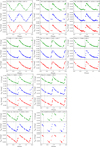 |
Fig. A.1. Light curves for the target stars in the Gaia bands. The vertical line shows the phase corresponding to the spectroscopic observations. For BF Ser, EK Del, and V716 Oph, the phases were taken from the literature. In particular, the line is only indicative for BF Ser and EK Del, for which multiple epochs of observations are available (see text for details). |
Appendix B: Abundances for the investigated ACEPs expressed as [X/Fe]
Abundances for the stars analysed in this work. All the data are expressed as [X/Fe] (dex).
Appendix C: Calculation of the integral of motion
To calculate the integral of motion, we adopted the Galpy package5 (Bovy 2015) adopting the McMillan17 potential (McMillan 2017). The calculation of the integral of motion requires positions, distances, proper motions, and RVs. For the GGCs, all these quantities are available in the fourth version of our globular cluster database6 based on Vasiliev & Baumgardt (2021), Baumgardt & Vasiliev (2021). Similarly, for the satellite of the MW, we used the Local Group and Nearby Dwarf Galaxies database7 based on the data published by McConnachie & Venn (2020) to obtain the integral of motion for 54 Local Group members.
For the ACEPs, positions and proper motions are from Gaia DR3. In the same catalogue, we found the average RVs (over many epochs) for eight stars (including EK Del, for which only the DR2 value is available), while for the remaining four stars (DR2 2976160827140900096, DR2 6498717390695909376, SHM2017 J000.07389-10.22146, and HE 2324-1255), we adopted the radial velocities measured from our spectra. Because the RV of a pulsating star can vary up to a few tenths of km/s, these RVs are less precise than those in the Gaia catalogues, but we do not expect that this significantly affects the derivation of the integral of motion. Calculating the distances of the ACEPs is a more complex task. First, we tried to use the Gaia EDR3-based distances from Bailer-Jones et al. (2021), but the parallaxes were too small and the relative error on the parallaxes too large for many stars (see Table 1), so that these distances substantially reflect the Galactic model used as prior. Therefore, we adopted a different approach. We assumed the PW relation in the Gaia bands for the ACEP_F in the LMC (the same data shown in Fig. 2) in the form published by Ripepi et al. (2023), but with the zero-point calibrated in absolute terms using the geometric distance of the LMC based on eclipsing binaries (18.477±0.026 mag, Pietrzyński et al. 2019). The adopted PW is WG = −1.687 − 3.080 × log P, where WG = G − 1.90 × (GBP − GRP) and P is the period. The period of ACEP_1O was fundamentalised using the relation log PF = log P1O + 0.13 (Caputo et al. 2004). The comparison of the absolute WG with the apparent one readily gives us the distances of the pulsators, which are listed in Table 1. As a final note, we confirmed that these distances agree perfectly with those by Bailer-Jones et al. (2021) for the closest stars in our sample, for instance, BF Ser and V716 Oph.
All Tables
Abundances for the stars analysed in this work. All the data are expressed as [X/Fe] (dex).
All Figures
|
Fig. 1. Position on the sky in Galactic coordinates for the nine targets observed in this work (magenta filled circles in the southern hemisphere). The three complementary stars taken from the literature are also shown (magenta filled circles in the northern hemisphere). For comparison, light blue dots display the position of all the ACEPs in the Gaia DR3 catalogue. |
| In the text | |
|
Fig. 2. Period–Wesenheit relation in the Gaia bands for the 11 ACEP_Fs (filled green circles) and one ACEP_1O (filled black circle, log P shifted by −0.01 to avoid overlap with F pulsators) in comparison with analoguous data for the LMC (red and blue dots represent ACEP_Fs and ACEP_1Os, respectively). To obtain the absolute Wesenheit magnitude for the LMC stars, we adopted the distance modulus by Pietrzyński et al. (2019). |
| In the text | |
|
Fig. 3. Excerpt from our UVES spectra for the nine ACEPs. The black and red lines show the data and the best-fitting synthetic spectra, respectively. Some lines are labelled in the figure, as is the iron abundance. In the right panel, we show the fit of the Na I doublet at 5889–5895 Å. It is possible to note the interstellar sodium lines in four out of nine stars, for which we accurately fit only the line profile of the stellar sodium. |
| In the text | |
|
Fig. 4. Abundances of sodium, magnesium, silicon, calcium, and titanium for the ACEPs (solid red points with error bars) in comparison with GGCs (yellow stars) and the GALAH MW data. |
| In the text | |
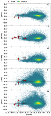 |
Fig. 5. As in Fig. 4, but for iron group and heavy elements: Sc,Cr, Ni, Y, Ba. |
| In the text | |
|
Fig. 6. Same as in Fig. 4, but for the comparison with three dSph hosting an extended intermediate-age population, namely Carina, Fornax and Leo I (see labels). |
| In the text | |
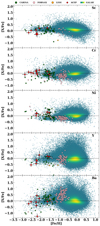 |
Fig. 7. As in Fig. 6, but for the Sc, Cr, Ni, Y, Ba. |
| In the text | |
|
Fig. 8. Same as in Fig. 4, but for the comparison with several dSph hosting a purely old population. Becaus of the high number of galaxies, we display all the data with the same colour for clarity (magenta). |
| In the text | |
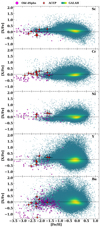 |
Fig. 9. As in Fig. 8, but for the Sc, Cr, Ni, Y, Ba. |
| In the text | |
|
Fig. 10. Same as in Fig. 4, but for the comparison with several UFDs. Because of the high number of galaxies, we display all the data with the same colour for clarity (green). |
| In the text | |
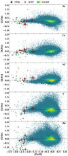 |
Fig. 11. As in Fig. 10, but for the Sc, Cr, Ni, Y, Ba. |
| In the text | |
|
Fig. 12. Histogram of individual [Na/Fe] abundances for stars belonging to 15 GGCs (red) and the investigated ACEPs (blue). The GGCs data are from Carretta et al. (2009b). |
| In the text | |
|
Fig. 13. Angular momentum in the z direction vs total energy of the orbit of the ACEP sample studied in this paper (filled red circles) in comparison with a sample of 166 GGCs (smaller filled light green circles) and of dwarf galaxies of the Local Group (smaller filled grey circles). To avoid confusion, the long identification names of some stars were abbreviated as follows: CRTS = CRTS J003041.3−441620; DR2_96 = DR2 2976160827140900096; HE_29 = HE 0114-5929; HE_55 = HE2324−1255; OGLE_006 = OGLE GAL-ACEP-006; SHM = SHM2017J000.07389−10.22146; DR2_24 = DR2 2648605764784426624; DR2_76 = DR2 6498717390695909376. |
| In the text | |
|
Fig. 14. Visual amplitude of the observed ACEPs as a function of the [Na/Fe] abundance. The solid line shows a linear regression to the data that does not include the three stars with low values of the [Si/Fe], [Ti/Fe] and [Sc/Fe] abundances (green symbols, see labels). In the labels, TW and Lit. indicate the nine stars that were studied spectroscopically in this paper and the three with spectroscopy from the literature, respectively. |
| In the text | |
|
Fig. 15. Sodium overabundances in RGB stellar models undergoing a rotation-induced deep-mixing process. The black lines refer to 1.2 M⊙ models, and the red line plots a 1.5 M⊙ model. The solid, long-dashed, and dotted lines represent cases in which the deep-mixing attains a maximum temperature of Tmax = 19, 23, and 27 MK, respectively. |
| In the text | |
|
Fig. A.1. Light curves for the target stars in the Gaia bands. The vertical line shows the phase corresponding to the spectroscopic observations. For BF Ser, EK Del, and V716 Oph, the phases were taken from the literature. In particular, the line is only indicative for BF Ser and EK Del, for which multiple epochs of observations are available (see text for details). |
| In the text | |
Current usage metrics show cumulative count of Article Views (full-text article views including HTML views, PDF and ePub downloads, according to the available data) and Abstracts Views on Vision4Press platform.
Data correspond to usage on the plateform after 2015. The current usage metrics is available 48-96 hours after online publication and is updated daily on week days.
Initial download of the metrics may take a while.