| Issue |
A&A
Volume 686, June 2024
|
|
|---|---|---|
| Article Number | A271 | |
| Number of page(s) | 12 | |
| Section | Cosmology (including clusters of galaxies) | |
| DOI | https://doi.org/10.1051/0004-6361/202347890 | |
| Published online | 19 June 2024 | |
Identifying frequency de-correlated dust residuals in B-mode maps by exploiting the spectral capability of bolometric interferometry
1
Université Paris Cité, CNRS, Astroparticule et Cosmologie, 75013 Paris, France
e-mail: regnier@apc.in2p3.fr
2
Università degli studi di Milano, Milano, Italy
3
INFN sezione di Milano, 20133 Milano, Italy
4
Université PSL, Observatoire de Paris, AstroParticule et Cosmologie, 75013 Paris, France
5
Waterloo Centre for Astrophysics, University of Waterloo, Waterloo, ON N2L 3G1, Canada
6
Department of Physics and Astronomy, University of Waterloo, Waterloo, ON N2L 3G1, Canada
7
Institut de Recherche en Astrophysique et Planetologie, Toulouse (CNRS-INSU), Toulouse Cedex 4, France
8
Universita di Roma, La Sapienza, Italy
9
National University of Ireland, Maynooth, Ireland
10
Università di Milano – Bicocca and INFN Milano-Bicocca, Milano, Italy
11
ITeDA-Mza.(CNEA, CONICET, UNSAM), Buenos Aires, Argentina
12
Instituto Argentino de Radioastronomía (CCT La Plata, CONICET; CICPBA; UNLP), Buenos Aires, Argentina
13
Consejo Nacional de Investigaciones Científicas y Técnicas (CONICET), Godoy Cruz 2290, Ciudad de Buenos Aires C1425FQB, Argentina
14
Facultad de Ciencias Astronómicas y Geofísicas, Universidad Nacional de La Plata, Paseo del Bosque, La Plata, B1900FWA Buenos Aires, Argentina
15
Universidad de Buenos Aires, Facultad de Ciencias Exactas y Naturales, Departamento de Física, Intendente Güiraldes 2160, Ciudad Universitaria, Ciudad de Buenos Aires C1428EGA, Argentina
Received:
6
September
2023
Accepted:
15
February
2024
Context. Astrophysical polarized foregrounds represent the most critical challenge in cosmic microwave background (CMB) B-mode experiments, requiring multifrequency observations to constrain astrophysical foregrounds and isolate the CMB signal. However, recent observations indicate that foreground emission may be more complex than anticipated. Not properly accounting for these complexities during component separation can lead to a bias in the recovered tensor-to-scalar ratio.
Aims. In this paper we investigate how the increased spectral resolution provided by band-splitting in bolometric interferometry (BI) through a technique called spectral imaging can help control the foreground contamination in the case of an unaccounted-for Galactic dust frequency de-correlation along the line of sight (LOS).
Methods. We focused on the next-generation ground-based CMB experiment CMB-S4 and compared its anticipated sensitivity, frequency, and sky coverage with a hypothetical version of the same experiment based on BI (CMB-S4/BI). We performed a Monte Carlo analysis based on parametric component separation methods (FGBuster and Commander) and computed the likelihood of the recovered tensor-to-scalar ratio, r.
Results. The main result is that spectral imaging allows us to detect systematic uncertainties on r from frequency de-correlation when this effect is not accounted for in the component separation. Conversely, an imager such as CMB-S4 would detect a biased value of r and would be unable to spot the presence of a systematic effect. We find a similar result in the reconstruction of the dust spectral index, and we show that with BI we can more precisely measure the dust spectral index when frequency de-correlation is present and not accounted for in the component separation.
Conclusions. The in-band frequency resolution provided by BI allows us to identify dust LOS frequency de-correlation residuals where an imager with a similar level of performance would fail. This creates the possibility of exploiting this potential in the context of future CMB polarization experiments that will be challenged by complex foregrounds in their quest for B-mode detection.
Key words: methods: data analysis / cosmic background radiation / inflation / submillimeter: ISM
© The Authors 2024
 Open Access article, published by EDP Sciences, under the terms of the Creative Commons Attribution License (https://creativecommons.org/licenses/by/4.0), which permits unrestricted use, distribution, and reproduction in any medium, provided the original work is properly cited.
This article is published in open access under the Subscribe to Open model. Subscribe to A&A to support open access publication.
1. Introduction
This paper addresses one of the burning questions currently concerning the cosmic microwave background (CMB) community: Are there reliable strategies to validate or invalidate a detection of primordial B modes in the presence of complex, polarized Galactic foregrounds? The scope of our paper is to investigate a possible solution that exploits the spectral imaging capability of an unconventional technique for CMB polarimetry, called bolometric interferometry (BI), applied to control interstellar dust foreground emission residuals.
The next generation of satellites, including Litebird (Hazumi et al. 2019) and the Probe of Inflation and Cosmic Origins (PICO; Hanany et al. 2019), and ground-based experiments, such as that conducted by the Simons Observatory (Ade et al. 2019) and CMB-S4 (Abazajian et al. 2022), aim at improving the constraint on the tensor-to-scalar ratio, r, at the level of 0.001 and below. The accurate removal of foreground and instrumental systematic effects is already the main limiting factor.
To improve foreground removal, modern experiments rely on multifrequency observations and improved models of astrophysical emissions. For example, many PySM1 (Thorne et al. 2017) models have been developed with the goal of simulating the effects of deviations from the single modified blackbody (MBB) emission conventionally assumed for the Galactic dust thermal emission. The models d5 and d7 take different dust grain compositions into account (Hensley & Draine 2017), while models d4 and d12 describe the dust emission as a sum of between two and six single MBBs along each line of sight (LOS; Finkbeiner et al. 1999; Martínez-Solaeche et al. 2018).
This article focuses on the d6 model (Vansyngel et al. 2018), which introduces LOS frequency de-correlation due to a frequency-varying polarization angle, which in turn is caused by a change in both the spectral energy distribution (SED) and the magnetic field orientation along the LOS (Tassis & Pavlidou 2015). This effect is usually quantified at the power spectra level by means of the correlation ratio, Rℓ, between two frequency maps (Planck Collaboration Int. L 2017). The most recent observational evidence of this effect comes from Planck Collaboration Int. L (2017), Planck Collaboration XI (2020), Pelgrims et al. (2021), and Ritacco et al. (2023) and could affect polarimetric and spectral calibration in the case of wide beam instruments (Masi et al. 2021) as well as bias the tensor-to-scalar ratio (McBride et al. 2023; Hensley & Bull 2018).
However, the d6 model mimics the effect of a frequency-varying polarization angle, without making any physical assumptions on the misalignment of the underlying magnetic field, by randomly sampling a frequency-varying multiplication factor from a Gaussian distribution that is later applied to the single MBB emission, using the parametric expression of the correlation ratio derived in Vansyngel et al. (2018). If dust does not behave as a simple MBB, as is usually assumed, but exhibits more complex spectral features, such as frequency de-correlation, we need a method for detecting the presence of foreground residuals in our results. This could be achieved by comparing results from different sky patches, as proposed by Aurlien et al. (2023), or by cross-checking with different component separation methods, such as parametric codes (Eriksen et al. 2006; Stompor et al. 2008), blind algorithms (Aumont & Macías-Pérez 2007), or codes based on moment expansion (Chluba et al. 2017; Vacher et al. 2022), some of which might be less sensitive to incorrect foreground modeling.
Another possibility, which we illustrate in this paper, is to use BI and its ability to discriminate frequencies in-band during data analysis. This allows us to achieve a spectral resolution of a few gigahertz2 and reanalyze the same data with different spectral configurations. A variation in the constraint on r between configurations suggests contamination in the tensor-to-scalar ratio due to component separation residuals.
In this paper we investigate the advantage of BI for foreground removal and characterization by comparing the performance in detecting dust frequency de-correlation of one of the most advanced experiments to date, CMB-S4, with a similar, hypothetical experiment based on BI, which we name CMB-S4/BI. We performed a Monte Carlo simulation starting from frequency maps, with or without band-splitting, and then applied parametric component separation using two different component separation codes: FGBuster (Stompor et al. 2008) and Commander (Eriksen et al. 2006, 2008). In the main body of this paper, we focus on FGBuster simulations, and we discuss the results obtained with Commander in Appendix B.
Because the aim of this article is to propose a new methodology, we did not perform an actual map-making process from the time-ordered data. We simulated the noise properties directly onto the reconstructed frequency maps and neglected the impact of instrumental systematic effects, such as an imperfect knowledge of the spectral response of the instrument, uncertainty regarding the half-wave plate angle, or the feed-horn positions. Such effects could reduce the ability to perform band-splitting during data analysis. However, BI offers a specific approach to controlling instrumental systematic effects, the self-calibration technique, which is inherited from radio interferometers (Bigot-Sazy et al. 2013).
The paper is organized as follows. In Sect. 2 we provide a brief introduction to BI (and references therein Hamilton et al. 2022). Section 3.1 describes the simulated sky models, instrumental configurations, and the Monte Carlo pipeline based on the FGBuster (Stompor et al. 2008) component separation code. In Sect. 3.2 we compare the results in terms of tensor-to-scalar ratio reconstructions from simulations with conventional foreground models and with unaccounted-for Galactic dust LOS frequency de-correlation. We also describe a machine learning classification used to assess the ability to detect residuals from foreground emissions in a single realization. In Appendix A we present the results obtained with FGBuster regarding the estimation of foreground parameters, and in Appendix B we discuss all the results obtained with Commander.
2. Bolometric interferometry in a nutshell
In this section we briefly describe the principles of BI, focusing on a specific feature of this technique, called spectral imaging, which is at the heart of our study. The interested reader can find more details on BI and spectral imaging in Hamilton et al. (2022), Mousset et al. (2022), whereas more information about the Q & U Bolometric Interferometer for Cosmology (QUBIC) experiment, currently the only one based on BI, and on its laboratory characterization can be found in Torchinsky et al. (2022), Piat et al. (2022), Masi et al. (2022), D’Alessandro et al. (2022), Cavaliere et al. (2022), and O’Sullivan et al. (2022).
Bolometric interferometry is a technique that combines the use of bolometers, which are state-of-the-art wide-band cryogenic detectors providing high sensitivity, with the advantage of precision control of systematic effects provided by the self-calibration technique, commonly used in radio-interferometry (Cornwell & Wilkinson 1981). The application to BI is detailed in Bigot-Sazy et al. (2013).
Figure 1 shows a schematic of the QUBIC instrument, highlighting the fundamentals of BI. The sky signal enters the cryostat through an aperture window and propagates through a series of filters, a step-rotating half-wave plate, a polarizing grid, and an array of paired back-to-back feed-horn antennas. The back horns directly illuminate an optical combiner, which focuses the radiation onto two focal planes through a dichroic plate.
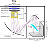 |
Fig. 1. Schematic of the QUBIC instrument, showing the principle of BI. The sky signal is received by an array of back-to-back horns and reimaged onto the bolometric focal planes, where the field interferes additively. A polarizer and a rotating half-wave plate make the instrument sensitive to linear polarization. |
When the instrument observes a distant point source along the optical axis an interference pattern forms on the two focal planes (see the top panel of Fig. 2). As a result, each focal plane element measures the sky signal convolved by a specific beam pattern, called the synthesized beam, shown in the bottom panel of Fig. 2. The constructive or destructive interference of the incoming signal defines a series of peaks and nulls, with properties that depend on the signal wavelength, λ, on the number of horns along the maximum axis of the antennas array, P, and on the separation between two consecutive horns, Δh, as follows (Mousset et al. 2022):
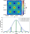 |
Fig. 2. Synthetized beam of QUBIC. Top panel: simulation of the interference pattern on the focal plane generated by a monochromatic point source. Bottom panel: azimuth cut of the theoretical synthesized beam (solid lines) at 140 GHz (blue line) and at 160 GHz (green line) for a detector at the center of the focal plane. Dashed lines represent the beam pattern of a single feed horn. The frequency-dependent position of the secondary peaks is clearly visible. |
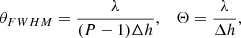
where θFWHM is the half power width of the peaks and Θ is the angular distance between the main peak and the first secondary peak.
Equation (1) demonstrates that the positions of the secondary peaks depend on λ. As an example, in the bottom panel of Fig. 2 we show a cut of the synthesized beam at a fixed azimuthal angle for two frequencies: 140 GHz and 160 GHz. Knowing how the multiple-peaked shape of the synthesized beam evolves with frequency allows us to recover the sky signal during data analysis at various frequencies within the physical band. This is possible as long as the two frequencies, ν1 and ν2, are far enough apart that the secondary peaks are well resolved. That is, we required  , which occurs for
  . We call this technique spectral imaging.
Our goal is to reconstruct maps of an extended source in polarization thereby computing the three Stokes parameters I, Q, and U at the same time. Because an extended source is a linear combination of point-sources, this reconstruction is possible but requires deconvolving from the multiple peaks of the synthesized beam, as well as relying on a half-wave plate modulation for polarization reconstruction. This problem can be solved thanks to a scanning strategy that allows information to be captured several times with various geometrical configurations3, and through an inverse problem approach that reconstructs unbiased maps of the three Stokes parameters in sub-bands within the physical band of the instrument (Mousset et al. 2022).
Consequently, the frequency dependence of the secondary peaks enables us to achieve a spectral resolution of a few gigahertz within the physical band. Furthermore, since spectral imaging occurs at the data analysis level, it allows us to reanalyze the same data with different spectral configurations, which can help us detect biases in the obtained results. This is a unique asset compared to traditional imagers, which would need several focal planes coupled to multichroic filters to achieve the same spectral performance, or to Fourier-transform spectrometers, which would suffer from a noise penalty related to not observing all frequencies simultaneously. In this context, our aim is to investigate how the increased spectral resolution provided by BI helps in controlling the contamination from Galactic foregrounds in the quest for primordial B-mode detection, with a special focus on the Galactic dust emission.
3. Dust de-correlation with bolometric interferometry and direct imaging
This paper aims to quantify the effect of various dust models with increasing complexity on the component separation results and demonstrate the benefits of spectral imaging in this regard. We focused, in particular, on the LOS frequency de-correlation of thermal dust, a phenomenon already observed in Planck data (Pelgrims et al. 2021).
To quantify dust de-correlation, we followed Planck Collaboration XI (2020) and used the quantity ℛℓ, defined in Eq. (2):
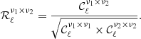
Here ℛℓ is the ratio between the crossed spectrum between two frequencies, ν1 and ν2, and the square root of the product of the auto-spectra at these same frequencies. This ratio is close to 1 for completely correlated thermal dust. In our sky simulations, we can increase or decrease the level of complexity in the thermal dust SED by tuning ℛℓ to a value farther or closer to one, thanks to the parametric expression of ℛℓ derived in Eq. (14) of Vansyngel et al. (2018).
To assess the potential of BI, we compared the component separation performance of CMB-S4 to a BI version of the same experiment that has the same sensitivity per unit bandwidth, but allowing for a higher spectral resolution through band-splitting using spectral imaging. In the following subsections, we present the methods used for this comparison.
3.1. Methods
3.1.1. Simulated sky
Our sky model contains the CMB plus synchrotron and dust emission foregrounds. We simulated the CMB using angular power spectra provided by the fgbuster package that are based on the latest Planck 2018 results4. We used the following two FITS files: (i) Cls_Planck2018_lensed_scalar.fits in which B modes are considered with r = 0 and lensing. (ii) Cls_Planck2018_unlensed_scalar_and_tensor_r1.fits in which B modes are considered with r = 1 and no lensing.
In our simulations, we used temperature and E-mode polarization spectra, which we denote as TT, EE, and TE. They are taken directly from file (i). The B-mode spectra, BB, were obtained by summing the BB spectra from file (i) and multiplying the sum by a lensing residual of 0.1; the BB spectrum from file (ii) was multiplied by the value of r (either 0 or 0.006). We note that such a simplified approach neglects the additional tensor contribution to the TT, TE, and EE spectra, but is sufficient in our case, as we only performed the likelihood analysis on the BB spectrum.
For the foregrounds we considered the following models5:
-
Model d0s0 assumes a single MBB emission for the thermal dust and a power-law emission for the synchrotron with no curvature, with constant dust spectral index across the sky, βd = 1.54, dust temperature, Td = 20 K, and synchrotron spectral index, βs = −3.
-
Model d1s1 is derived from the Planck data post-processed with the Commander code (Planck Collaboration X 2016) for the dust emission, while the synchrotron emission is taken from the Haslam data at 408 MHz in Remazeilles et al. (2015) and Haslam et al. (1982). The thermal dust emission is modeled as a MBB with spatially varying temperature and spectral index projected on the sky, while the synchrotron emission is modeled as a power law with spatially varying spectral index with no curvature.
-
Model d6s1 is derived from d1s1 with the introduction of LOS frequency de-correlation in the dust emission following the statistical approach described in Eq. (14) of Vansyngel et al. (2018).
Whereas models d0s0 and d1s1 are fixed realizations, the model d6s1 results in a random realization of the SED. For each simulated frequency, the MBB emission is multiplied by a randomly sampled de-correlation factor that mimics the effect of a frequency-varying polarization angle without making any physical assumptions on the underlying Galactic magnetic field. The magnitude of the de-correlation factor is governed by the correlation length, ℓcorr, a parameter that can be set in PySM. Figure 3 displays the dispersion of various SED realizations as a function of ℓcorr, showing that the dispersion increases with a shorter correlation length.
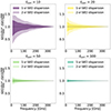 |
Fig. 3. Dispersion of the dust SED for different correlation lengths of the PySM d6 model normalized by the single MBB emission (d1 model). The colored areas represent the statistical deviation from a MBB for a given correlation length, evaluated over 500 realizations. |
In our simulations, we explored the effect of dust LOS frequency de-correlation with a level of de-correlation consistent with current observations. Specifically, the range of correlation lengths used in our study was ℓcorr ≥ 10, which corresponds to a de-correlation level below 5% for all the simulated frequencies. This configuration represents a conservative scenario with respect to the de-correlation level measured by Planck (Planck Collaboration Int. L 2017; Planck Collaboration XI 2020) in the same multipole range considered in our work (ℓ ≤ 300; see Fig. 4 for a comparison with Planck estimates).
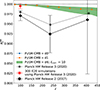 |
Fig. 4. Correlation ratio measured by Planck from the Half Mission (HM) maps at 217 GHz and 353 GHz, compared to the simulated ratio using PySM dust and CMB templates at the same frequencies. The blue and orange dots represent the expected Rℓ for the CMB and a single MBB dust emission, with constant (d0) or varying pixel-by-pixel (d1) spectral indices, respectively. Note that the dots are so close that they overlap in the figure. The green envelope shows the range of Rℓ obtained from 500 realizations of dust LOS frequency de-correlation with ℓcorr = 10. The black dots are from Fig. 2 of Planck Collaboration Int. L (2017), the gray dots are from Fig. B.2 of Planck Collaboration XI (2020), and the red point is obtained from the values in the middle plot of the second row in Fig. 18 of Planck Collaboration XI (2020). |
3.1.2. Instrument models
The first instrument considered in our analysis is CMB-S4 (Abazajian et al. 2022), which will observe at 9 different frequencies in the 20–280 GHz range to constrain both synchrotron and thermal dust emissions. The goal of CMB-S4 will be the detection of r at the level r > 0.003 with more than 5σ.
The second instrument is a version of CMB-S4 based on BI (CMB-S4/BI), where each of the bolometer-based frequency bands, Δνi (i.e., above 85 GHz), can be subdivided into nsub sub-bands of width

If we now consider m frequency bands of CMB-S4, each one subdivided into nsub sub-bands in CMB-S4/BI, we can calculate the sensitivity in each sub-band as
where σj is the CMB-S4 sensitivity in the jth sub-band within ith physical band, nsub is the number of sub-bands and ε is a parameter introduced to account for the sub-optimality of BI (for further details about BI sub-optimality, see Mousset et al. 2022).
We made two approximations regarding the instrument models:
-
The noise is always assumed to be white, although, in CMB-S4/BI, we added the multiplicative term ε to account for the sub-optimality of BI. We know that the noise of a bolometric interferometer is not entirely white, and this calls for specific component separation techniques able to deal with correlated noise. These techniques are currently under development within the QUBIC Collaboration.
-
We neglected the angular resolution of the optical beam to be consistent with the CMB-S4 reference paper. The angular resolution of a traditional imager, such as CMB-S4, is set by the aperture of the telescope, whereas in the BI case this is set by the largest distance between horns. Although the contribution of the physical beam affects the final sensitivity of both instruments, it should not impact the generality of our results.
Figure 5 shows the bandwidths and sensitivities of some of the tested experimental configurations. For each CMB-S4 frequency interval above 85 GHz, we studied seven configurations of CMB-S4/BI, with nsub ranging from 2 to 8. Increasing the number of sub-bands results in a sensitivity degradation, as indicated in Eq. (4), with ε ranging between 20% and 60%, according to Mousset et al. (2022). Since we focused on dust de-correlation, we did not subdivide the synchrotron frequency bands; the first three intervals of the various configurations thus overlap. We note that because the simulated CMB-S4 sky patch is centered far from the Galactic plane, we expect the correlations between dust and synchrotron to be negligible for the scope of our study, in accordance with the results from Krachmalnicoff et al. (2018) and Planck Collaboration Int. L (2017).
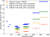 |
Fig. 5. Polarization sensitivity of CMB-S4 and three examples of CMB-S4/BI, with nsub = 3, 5, and 7, respectively. Note that the bands of the three lowest-frequency channels are identical for all the instruments. Because our study focuses on dust de-correlation, we chose not to split the bandwidths of the synchrotron channels. |
We emphasize that because this band-splitting is performed at the data analysis level, one can explore various values of the number of sub-bands nsub with the same dataset. Studying the evolution of the resulting constraints as a function of nsub is the core of this study.
3.1.3. Simulation pipeline
We describe here the simulation pipeline for the Monte Carlo analysis that we performed using the FGBuster parametric component separation code. In Appendix B.1 we report the same information regarding the simulations performed with Commander. In the FGBuster analysis, we simulated the anticipated CMB-S4 patch, which is a 3%, circular sky patch centered in RA, Dec = (0° , − 45° ).
We considered eight instrument configurations (see also Fig. 5): The CMB-S4 configuration (parametrized following Abazajian et al. 2022) and seven versions of CMB-S4/BI, obtained by subdividing each frequency band. We then applied component separation and analyzed the cross-spectra of the resulting maps using a uniform binning (see Table 1 for a summary of the simulation setup).
Parameters used for analyzing simulations with FGBuster for all dust models.
For each instrument configuration, the overall analysis chain followed these steps:
-
Generate a CMB realization as described at the beginning of Sect. 3.1.1.
-
Generate a noise realization for each frequency channel in the considered instrument configuration.
-
Add the CMB and the noise to the foreground maps generated as described in Sect. 3.1.1.
-
Apply component separation to the input maps. In some cases we assumed the same model used to generate the input case. In others, we assumed a different model in order to mimic a realistic situation in which the actual foregrounds are not 100% known and one might assume a model that does not completely describe reality.
-
Perform a cross-spectra analysis between two noise realizations (each with half the exposure time) to recover the tensor-to-scalar ratio, r. We calculated angular power spectra using the NaMaster6 code (Alonso et al. 2019) with an apodization radius of 4°.
In Table 2 we list the various cases studied in this work. Each case was simulated with all the instrument configurations described in Sect. 3.1.2 and Fig. 5.
Cases analyzed in this work.
Component Separation. We performed parametric component separation modeling on our data as follows:
where p is the pixel index, dp and np are vectors representing the data and noise measured by the instrument frequency channels, sp is a vector containing the “true” sky values at the same frequencies, and A is a mixing matrix that contains information about the sky components (CMB, synchrotron, and interstellar dust). In our simulations, we considered the dust temperature as a known parameter, Td = 20 K. Thus, the only unknown parameters for synchrotron and dust emissions were their spectral indices, βs and βd.
FGBuster solves for the best spectral indices, βs and βd, given the data, dp, and the noise covariance matrix, N, following the spectral likelihood approach of Stompor et al. (2008). In order to cope with computational constraints (processing time and computer memory) and keep the same parameters as in Abazajian et al. (2022), we used a double pixelization scheme in our component separation: A fine resolution of Nside = 256 for the pixels of the reconstructed maps, and a coarse resolution of Nside = 8 (corresponding to a super-pixel resolution of about 7°) for the spectral indices. In other words, the spectral indices are kept constant on larger pixels compared to those of the reconstructed maps. This approach introduces a slight bias on r, as demonstrated and addressed in Sect. 3.2.1. However, this bias does not alter the general validity of our results.
Tensor-to-scalar ratio estimation. The main goal of our study is to assess how residuals caused by biased estimates of foreground parameters impact the reconstruction of the tensor-to-scalar ratio, r, which is the main parameter characterizing the primordial CMB B modes.
We write the likelihood on r using a Gaussian approximation (Hamimeche & Lewis 2008):

where  and
and  are the measured and theoretical angular power spectra,
  is the inverse of the sum of the noise and sample variance-covariance matrices, and ℒ(r) is the likelihood on r. The theoretical angular power spectrum,
  , includes the contribution of the 10% lensing residual that we assumed throughout the study. Therefore, the only free parameter is the tensor-to-scalar ratio, r, which we varied with a flat prior in the range [−1, 1]. Although allowing for negative values of r is unphysical, we opted for this more general approach because it has the benefit of highlighting potential biases due only to differing observational methodologies.
This work explores what happens when dust is more complex than anticipated. In order to do so, we performed component separation assuming a simple model for dust, namely d1s1, but applied to data simulated with the d6s1 model. In such cases, incorrect dust modeling leads to residuals in the clean CMB maps.
We then constructed the log-likelihood for r assuming dust to be well modeled by d1s1 using the noise covariance matrix in Eq. (6), Nℓ, ℓ, obtained from simulations without frequency de-correlation in the dust emission. Such a covariance matrix does not incorporate the variance arising from the dust SED de-correlation so that the bias on r appears with a high significance, which is precisely the effect we want to study.
After a large number of realizations of d6s1, we see a distribution that shows the large spread in the possible values of r, which would be incorrectly considered a measure of high significance because we assumed a simple model for dust. We used the same scheme for all of our instrument configurations (from a classical imager to a bolometric interferometer with a number of sub-bands) so that we could explore whether the extra spectral information provided by BI allows us to identify if the “clean” CMB maps after component separation are indeed clean or are contaminated by dust residuals.
3.2. Results
3.2.1. Reconstruction of the tensor-to-scalar ratio, r
Here we discuss the results of our FGBuster simulations in terms of the reconstruction of the tensor-to-scalar ratio, r. The performance in terms of foreground reconstruction is discussed in Appendix A (FGBuster simulations), whereas the Commander simulations are presented in Appendix B.2.
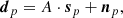
The four panels in Fig. 6 show the histograms of the maximum likelihood values of r computed from Eq. (6) for each iteration of the Monte Carlo chain. Each panel shows the result for one of the simulated sky models as a function of nsub. The top-left panel shows the CMB with rinput = 0 and d0s0 foregrounds. The top-right panel shows the CMB with rinput = 0 and d1s1 foregrounds. The bottom-left panel shows the CMB with rinput = 0.006 and d1s1 foregrounds. The bottom-right panel shows the CMB with rinput = 0 and d6s1 foregrounds with ℓcorr = 10.
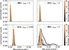 |
Fig. 6. Normalized histograms of the maximum likelihood values of r as a function of the number of sub-bands. Top left: model d0s0 with rinput = 0. Top right: model d1s1 with rinput = 0. Bottom left: model d1s1 with rinput = 0.006. Bottom right: model d6s1 with ℓcorr = 10 and rinput = 0. |
The histograms are normalized to the maximum count value and smoothed with a kernel density estimator of width equal to one-fourth of the standard deviation of the histogram. The histograms extend to negative r values because we computed the posterior likelihood over a range of r that includes negative values in order to avoid a sharp truncation of the likelihood at r = 0. A more detailed discussion of each of the four cases follows below.
Top-left panel. Here we have the CMB with rinput = 0 and d0s0 foregrounds. In this case, the reconstructed r does not depend on nsub and there is a small bias due to an E → B mode leakage caused by the power spectra computation on a sky patch, where the spherical harmonics are no longer orthogonal. This bias could be mitigated by increasing the apodization radius of the mask at the expense of a smaller effective sky fraction (< 3%). This optimization, however, is outside the scope of the paper.
Top-right panel. Here we have the CMB with rinput = 0 and d1s1 foregrounds. Also in this case we see that the reconstructed r does not depend on nsub, even if the complexity of the dust emission is higher (the dust spectral index varies in the sky). However, here we observe a slightly larger bias in r with respect to the d0s0 case, caused by the aforementioned leakage and also by the difference in pixel size of the reconstructed spectral indices maps (Nside = 8) compared to the input sky (Nside = 256).
Bottom-left panel. Here we have the CMB with rinput = 0.006 and d1s1 foregrounds. This case is similar to the previous one, the only difference being the value of rinput.
Bottom-right panel. Here we have the CMB with rinput = 0 and d6s1 foregrounds fitted with the d1s1 model. The histograms show that fitting with a model that does not account for frequency de-correlation produces distributions that are larger for smaller values of nsub. Also, the mean value of the reconstructed r obtained from such distributions varies and becomes smaller as nsub increases.
Figure 7 shows the average r and standard deviation computed from the histograms of Fig. 6 as a function of nsub. This result represents the range of r from which we expect to sample our measurement when performing CMB observations.
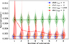 |
Fig. 7. Average maximum likelihood value of r and the standard deviation as a function of the number of sub-bands in the case of unaccounted-for dust frequency de-correlation (model d6s1 with ℓcorr = 10 and r = 0) compared to two cases of no de-correlation (model d1s1): r = 0 and r = 0.006. On top of the average r values and their standard deviation, we have overplotted the shape of the distribution as a “violin plot.” Note that for the d6 case the distribution is asymmetric for small nsub, so that the average is not centered on the distribution. |
We note that since the error bar is the standard deviation, we assume it to be symmetrical. Moreover, in the d6s1 case the histogram is unsymmetrical, and therefore the average r is not centered with the distribution.
The blue, orange, and green curves refer to the case in which we fit the same dust model used to simulate the input sky. In these three cases, the recovered r does not depend on nsub, as one would expect for a detection not contaminated by foregrounds. The difference between the recovered r with respect to rinput that we see in all three cases is caused by the E → B leakage and pixel size effects discussed above.
The red curve refers to the case in which the input sky contains dust emission with frequency de-correlation while component separation was performed ignoring this feature, assuming the d1s1 model. In this case, the increase in the number of frequency maps provided by BI allows us to better constrain the spectral indices, thus reducing the bias as the number of sub-bands increases. On average, a classical imager (represented by nsub = 1) would measure r ∼ 0.008 while a bolometric interferometer would see this estimate reducing by increasing nsub. This indicates that the first value of r is an artifact due to the presence of residual dust emission.
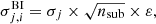
Finally, Fig. 8 shows a summary of the average r and standard deviation for all the simulated dust models with rinput = 0, including various correlation lengths for the d6s1 case: ℓcorr. = 10, 13, 16, 19, 100. For the sake of simplicity, we only show four instrument configurations: CMB-S4 and CMB-S4/BI with three, five, and seven sub-bands. As one can see, the advantage of BI in diagnosing foreground residuals, and therefore decreasing the bias on r, is maintained even in the case of smaller levels of dust frequency de-correlation. As expected, in the limit of ℓcorr. = 100 the result is compatible with the case of a single MBB (model d1s1).
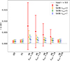 |
Fig. 8. Summary of the average maximum likelihood value of r and the standard deviation for an input r = 0 and all the simulated foreground models (d0s0, d1s1, and several ℓcorr cases of d6s1). Note that we assume symmetric error bars. |
3.2.2. Identifying foreground residuals on a single realization
We used machine learning to test the ability of BI to detect foreground residuals that may be present when the assumed foreground model is different from that describing the actual sky emission. That might occur, for example, if one assumes a d1s1 model when the sky is described by a d6s1 model. Therefore, we explored the possibility that two results – one contaminated by foreground residuals and the other not, but both producing the same average reconstructed r for an imager – can be correctly classified as “contaminated” or “not contaminated” (described by the case in which we do not split the physical band into sub-bands).
This ability is a key issue when an experiment detects a tensor-to-scalar ratio that is significantly different from zero. In this case, there is only one realization (i.e., the actual measurement) to understand whether there are unknown systematic effects biasing the value beyond the uncertainty set by the noise plus the known systematic effects.
We carried out this test by performing a machine learning classification based on a simple gradient-boosted decision tree (a GradientBoostingClassifier from the scikit-learn Python library7) according to these steps:
-
Produce 500 sky realizations with r = 0.0068 in which the sky is generated with d1s1 and fitted with the same model (we call this dataset d1-d1). This dataset is labeled as clean.
-
Produce 500 simulations with r = 0, in which the sky is generated with d6s1 (ℓcorr = 10) and fitted with d1s1 (we call this dataset d6-d1). This dataset is labeled as contaminated.
-
For each simulation, and for each value of nsub, calculate a normalized reconstructed r and its uncertainty normalized by what is found with nsub = 1, expressed by the following two quantities: ρ(nsub) = r(nsub)/r(nsub = 1) and σρ(nsub) = σ(r(nsub))/r(nsub = 1) (“training” dataset), both with a clean or contaminated label, depending on the model used as an input. These quantities are those that discriminate whether we have foreground residuals or not. If ρ ≠ 1, it means that the detection depends on the number of sub-bands and, therefore, is likely to be affected by foreground residuals.
-
Train the network with 250 (d1s1, r = 0.006) and 250 (d6s1, r = 0) randomly selected realizations from the training dataset (using 100 cross-validation subsets).
-
Calculate ρ(nsub) and σρ(nsub) for the remaining 250 (d1s1, r = 0.006) and 250 (d6s1, r = 0) simulations (“test” dataset).
-
Feed the trained network with the values calculated in step 5 to test its ability to classify the simulations as clean (constant ρ(nsub)) or contaminated (variable ρ(nsub)).
The result of this procedure is the so-called confusion matrix, that is, a matrix that compares the results from the classification predicted by the algorithm with the true one as shown in Fig. 9. The performance of our classifier is as follows (we adopted the convention “clean=negative” and “contaminated=positive”):
-
True negative rate very close to 1, indicating that the realizations with no dust residuals (dataset d1-d1 with r = 0 and r = 0.006) displayed a constant ratio ρ(nsub) and were correctly classified as clean.
-
True positive rate very close to 1, indicating that the realizations with dust residuals (dataset d6-d1 with r = 0), displayed a variable ratio ρ(nsub) and were correctly classified as contaminated.
-
Low false negative rate of 2.9%±1.6%, indicating a very low percentage of realizations with dust residuals that were wrongly classified as clean. This is a very important figure of merit that we want to minimize.
-
Low false positive of 1.2%±0.3%, indicating a very low percentage of realizations without dust residuals that were wrongly classified as contaminated.
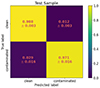 |
Fig. 9. Confusion matrix representing our ability to classify between our simulated datasets with dust frequency de-correlation (contaminated) or without (clean) using the measurements of r as a function of nsub. We observe that the fraction of false negatives (contaminated dataset incorrectly classified as clean) is close to zero. |
Such a high classification performance demonstrates that BI, with its capability to measure r in several sub-bands, is a promising solution to identify residuals in the clean CMB maps arising from LOS frequency de-correlation in the dust emission. In such a case, a classical imager lacks the frequency resolution to identify this contamination, leading to a systematic uncertainty in the reconstructed r that is well above the target sensitivity of CMB-S4.
4. Conclusions
In this paper we have shown how BI has the potential to detect systematic effects caused by interstellar dust in CMB polarization measurements when LOS frequency de-correlation is present in dust emission and is not accounted for in parametric component separation algorithms. We know that there are ways for imagers to mitigate the problem of not precisely knowing the foreground emission, for example through cross-checking with different component separation methods, such as blind ones (Aumont & Macías-Pérez 2007), or codes based on the moment expansion (Chluba et al. 2017; Vacher et al. 2022), which might be less sensitive to incorrect foreground modeling. However, in this paper we propose a new approach based on a different instrument architecture called BI. An instrument based on BI can be used as an independent verification of future claims of a B-mode detection by exploiting the superior purity of the r measurement made possible by the increased spectral resolution.
We carried out simulations with two component separation codes (FGBuster, discussed in the main text, and Commander, discussed in Appendix B), reconstructing the tensor-to-scalar ratio, r, from simulated skies containing CMB, synchrotron and dust emission, and instrumental noise. For the dust emission, we used three models of increasing complexity, one of which contains frequency de-correlation.
We compared two instrument models, CMB-S4 and CMB-S4/BI, the latter a modified version of CMB-S4 that accounts for the possibility of splitting each physical frequency band into a variable number of sub-bands that can be chosen during data analysis. This feature, which is unique to BI, allows us to assess whether a measurement of r is biased by dust emission residuals or not. While a Fourier-transform spectrometer can be used to increase spectral resolution, it would suffer a greater noise penalty compared to BI because it cannot observe all frequencies simultaneously.
Our results are consistent for the two codes and show that with no frequency de-correlation, the two instruments perform equally well (the final precision and systematic uncertainty on r are similar). If de-correlation is present, and it is not accounted for in the component separation, then an imager such as CMB-S4 would measure a biased value of r. This bias can be reduced with CMB-S4/BI by reanalyzing the same data after splitting the band into an increasing number of sub-bands.
The decrease in the measured r with the number of sub-bands, nsub, clearly indicates the presence of a dust-induced systematic effect, given that without dust residuals the detected r does not change with nsub. In such a situation, a classical imager would have no means of classifying the measurement as clean or “biased”. We also tested the ability to detect biased r measurements using a machine learning approach, and we verified that assessing the variation in the r measurement versus nsub allowed us to classify clean and biased measurements with a rate ≳97%.
In the future we will test this technique using more realistic situations (including representative noise, optical effects, and uncertainty on the knowledge of the instrumental spectral response). We will also assess the performance using various dust models and explore new techniques of component separation, which will allow us to separate signals by taking instrumental effects into account in a more comprehensive and representative way.
Some level of in-band frequency sensitivity can actually be achieved with traditional imagers by using the small variations in the spectral properties of different detectors. This was successfully applied to map the CO emission line (Planck Collaboration XVI 2014).
Spectra can be accessed at https://github.com/fgbuster/fgbuster/tree/master/fgbuster/templates
See https://pysm3.readthedocs.io/en/latest/#models for more details about the models.
The value of r = 0.006 was chosen so that the average reconstructed r matched the bias that would be obtained from a map with CMB with r = 0 and d6s1 foregrounds removed assuming a d1s1 model with a single reconstructed sub-band (see Fig. 7).
Available in the CAMB documentation (https://camb.readthedocs.io/en/latest/CAMBdemo.html).
Acknowledgments
QUBIC is funded by the following agencies. France: ANR (Agence Nationale de la Recherche) contract ANR-22-CE31-0016, DIM-ACAV (Domaine d’Intérêt Majeur-Astronomie et Conditions d’Apparition de la Vie), CNRS/IN2P3 (Centre national de la recherche scientifique/Institut national de physique nucléaire et de physique des particules), CNRS/INSU (Centre national de la recherche scientifique/Institut national des sciences de l’Univers). Italy: CNR/PNRA (Consiglio Nazionale delle Ricerche/Programma Nazionale Ricerche in Antartide) until 2016, INFN (Istituto Nazionale di Fisica Nucleare) since 2017. Argentina: MINCyT (Ministerio de Ciencia, Tecnología e Innovación), CNEA (Comisión Nacional de Energía Atómica), CONICET (Consejo Nacional de Investigaciones Cientìficas y Técnicas). S. Paradiso acknowledges support from the Government of Canada’s New Frontiers in Research Fund, through grant NFRFE-2021-00595. The authors want to thank Alexandre Boucaud for valuable advices about Machine Learning.
References
- Abazajian, K., Addison, G. E., Adshead, P., et al. 2022, ApJ, 926, 54 [CrossRef] [Google Scholar]
- Ade, P., Aguirre, J., Ahmed, Z., et al. 2019, J. Cosmol. Astropart. Phys., 2019, 056 [Google Scholar]
- Alonso, D., Sanchez, J., & Slosar, A. 2019, MNRAS, 484, 4127 [Google Scholar]
- Aumont, J., & Macías-Pérez, J. F. 2007, MNRAS, 376, 739 [CrossRef] [Google Scholar]
- Aurlien, R., Remazeilles, M., Belkner, S., et al. 2023, J. Cosmol. Astropart. Phys., 06, 034 [CrossRef] [Google Scholar]
- Bigot-Sazy, M.-A., Charlassier, R., Hamilton, J., Kaplan, J., & Zahariade, G. 2013, A&A, 550, A59 [NASA ADS] [CrossRef] [EDP Sciences] [Google Scholar]
- Cavaliere, F., Mennella, A., Zannoni, M., et al. 2022, J. Cosmol. Astropart. Phys., 2022, 040 [CrossRef] [Google Scholar]
- Chluba, J., Hill, J. C., & Abitbol, M. H. 2017, MNRAS, 472, 1195 [NASA ADS] [CrossRef] [Google Scholar]
- Cornwell, T. J., & Wilkinson, P. N. 1981, MNRAS, 196, 1067 [NASA ADS] [Google Scholar]
- D’Alessandro, G., Mele, L., Columbro, F., et al. 2022, J. Cosmol. Astropart. Phys., 2022, 039 [CrossRef] [Google Scholar]
- Eriksen, H. K., Dickinson, C., Lawrence, C. R., et al. 2006, ApJ, 641, 665 [CrossRef] [Google Scholar]
- Eriksen, H. K., Jewell, J. B., Dickinson, C., et al. 2008, ApJ, 676, 10 [Google Scholar]
- Finkbeiner, D. P., Davis, M., & Schlegel, D. J. 1999, ApJ, 524, 867 [NASA ADS] [CrossRef] [Google Scholar]
- Hamilton, J. C., Mousset, L., Battistelli, E. S., et al. 2022, J. Cosmol. Astropart. Phys., 2022, 034 [Google Scholar]
- Hamimeche, S., & Lewis, A. 2008, Phys. Rev. D, 77, 103013 [NASA ADS] [CrossRef] [Google Scholar]
- Hanany, S., Alvarez, M., Artis, E., et al. 2019, PICO: Probe of Inflation and Cosmic Origins, BAAS, 51, 194 [Google Scholar]
- Haslam, C. G. T., Salter, C. J., Stoffel, H., & Wilson, W. E. 1982, A&AS, 47, 1 [NASA ADS] [Google Scholar]
- Hazumi, M., Ade, P., Akiba, Y., et al. 2019, J. Low Temp. Phys., 194 [Google Scholar]
- Hensley, B. S., & Bull, P. 2018, ApJ, 853, 127 [NASA ADS] [CrossRef] [Google Scholar]
- Hensley, B. S., & Draine, B. T. 2017, ApJ, 836, 179 [NASA ADS] [CrossRef] [Google Scholar]
- Krachmalnicoff, N., Carretti, E., Baccigalupi, C., et al. 2018, A&A, 618, A166 [NASA ADS] [CrossRef] [EDP Sciences] [Google Scholar]
- Lewis, A., Challinor, A., & Lasenby, A. 2000, ApJ, 538, 473 [Google Scholar]
- Martínez-Solaeche, G., Karakci, A., & Delabrouille, J. 2018, MNRAS, 476, 1310 [Google Scholar]
- Masi, S., de Bernardis, P., Columbro, F., et al. 2021, ApJ, 921, 34 [NASA ADS] [CrossRef] [Google Scholar]
- Masi, S., Battistelli, E. S., de Bernardis, P., et al. 2022, J. Cosmol. Astrophys. Phys., 2022, 038 [Google Scholar]
- McBride, L., Bull, P., & Hensley, B. S. 2023, MNRAS, 519, 4370 [NASA ADS] [CrossRef] [Google Scholar]
- Mousset, L., Gamboa Lerena, M. M., Battistelli, E. S., et al. 2022, J. Cosmol. Astrophys. Phys., 2022, 035 [Google Scholar]
- O’Sullivan, C., de Petris, M., Amico, G., et al. 2022, J. Cosmol. Astrophys. Phys., 2022, 041 [Google Scholar]
- Pelgrims, V., Clark, S. E., Hensley, B. S., et al. 2021, A&A, 647, A16 [NASA ADS] [CrossRef] [EDP Sciences] [Google Scholar]
- Piat, M., Stankowiak, G., Battistelli, E. S., et al. 2022, J. Cosmol. Astrophys. Phys., 2022, 037 [Google Scholar]
- Planck Collaboration XVI. 2014, A&A, 571, A13 [NASA ADS] [CrossRef] [EDP Sciences] [Google Scholar]
- Planck Collaboration X. 2016, A&A, 594, A10 [NASA ADS] [CrossRef] [EDP Sciences] [Google Scholar]
- Planck Collaboration XI. 2020, A&A, 641, A11 [NASA ADS] [CrossRef] [EDP Sciences] [Google Scholar]
- Planck Collaboration Int. L. 2017, A&A, 599, A51 [NASA ADS] [CrossRef] [EDP Sciences] [Google Scholar]
- Remazeilles, M., Dickinson, C., Banday, A. J., Bigot-Sazy, M. A., & Ghosh, T. 2015, MNRAS, 451, 4311 [NASA ADS] [CrossRef] [Google Scholar]
- Ritacco, A., Boulanger, F., Guillet, V., et al. 2023, A&A, 670, A163 [NASA ADS] [CrossRef] [EDP Sciences] [Google Scholar]
- Stompor, R., Leach, S., Stivoli, F., & Baccigalupi, C. 2008, MNRAS, 392, 216 [Google Scholar]
- Tassis, K., & Pavlidou, V. 2015, MNRAS, 451, L90 [NASA ADS] [CrossRef] [Google Scholar]
- Thorne, B., Dunkley, J., Alonso, D., & Næss, S. 2017, MNRAS, 469, 2821 [Google Scholar]
- Torchinsky, S. A., Hamilton, J. C., Piat, M., et al. 2022, J. Cosmol. Astrophys. Phys., 2022, 036 [Google Scholar]
- Vacher, L., Aumont, J., Montier, L., et al. 2022, A&A, 660, A111 [NASA ADS] [CrossRef] [EDP Sciences] [Google Scholar]
- Vansyngel, F., Boulanger, F., Ghosh, T., et al. 2018, A&A, 618, C4 [NASA ADS] [CrossRef] [EDP Sciences] [Google Scholar]
Appendix A: Reconstruction of foregrounds parameters
In the main part of our paper we focus on the reconstructed tensor-to-scalar ratio, r, as it is the main quantity of interest. The level of systematic uncertainties in the reconstructed r, however, depends on the reconstructed foreground spectral parameters and distributions. Thus, in this appendix we focus on the distribution of the foregrounds spectral indices after component separation.
In Fig. A.1 we show the normalized histograms of the difference between the reconstructed and input dust and synchrotron spectral indices, Δβd, Δβs for the following three models: d0s0 (top row), d1s1 (middle row), d6s1 (bottom row), all with rinput = 0. Each histogram does not correspond to a particular pixel but contains values from the sky patch.
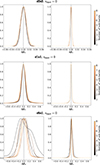 |
Fig. A.1. Reconstruction of foregrounds spectral indices. Top: Model d0s0, rinput = 0. Middle: Model d1s1, rinput = 0. Bottom: Model d6s1, rinput = 0. |
In the case of d0s0, the model assumes a constant spectral index all over the sky. Therefore, we expect unbiased estimates with a standard deviation related to the noise in the input frequency maps. The results shown in the top row of Fig. A.1 confirm this expectation as we observe no bias on the reconstructed spectral indices. We note that the standard deviation slightly increases with the number of sub-bands, nsub, because of the slight sub-optimality inherent to spectral-imaging (parametrized by ε in Eq. 4; see Mousset et al. 2022).
When spectral indices vary across the sky, as in d1s1, we expect biases in the reconstructed spectral indices because we only reconstructed the spectral indices on relatively large sky pixels (Nside = 8), while the input sky was simulated with spectral indices that vary among smaller pixels (Nside = 256). Consequently, averaging multiple spectral indices in large pixels introduces a bias to the reconstructed spectral index. This bias is responsible for foreground residuals in the CMB maps obtained after component separation and produces the bias on r observed in Figs. 6 and 7.
This is shown in the middle row of Fig. A.1. The bias due to spatial de-correlation appears as an enlarged spread of the distribution with respect to the d0s0 case (note the increased scale of the x-axis in the middle row compared to the top row). Also in this case we observe an increase in standard deviation with nsub caused by the sub-optimality related to spectral imaging.
Finally, in the case of frequency de-correlation in the dust emission (d6s1 model), spectral indices are no longer an accurate description of the dust spectral behavior. As a result, if we reconstruct βd using a d1s1 model, we expect a much larger bias. We note that the comparison between input and reconstructed spectral indices is done using the template map of βd (Planck Collaboration X 2016) that was used as an input for the d6s1 model. It is clear, however, that in the case of d6s1, the comparison between the input and recovered spectral indices is less meaningful than in the simpler models. In this case, one is more interested in the residuals found in the clean CMB maps, discussed in the main text of this article. In this case, the increase in spectral resolution provided by spectral imaging supplies extra information, allowing us to reduce this bias. This is confirmed by the results shown in the bottom row of Fig. A.1. First, we see a much larger spread in the histograms compared to the other two cases. Second, we see that the spread reduces significantly by increasing nsub. In this case, the benefit from spectral imaging more than balances out the sub-optimality effect and allows us to reduce the bias on the reconstructed spectral index, which then reduces the bias on r, as shown in Fig. 7.
Appendix B: Simulations with Commander
B.1. Simulation pipeline
We describe here the simulation pipeline for the analysis performed using the Commander code (Eriksen et al. 2006, 2008). We generated 100 CMB power spectra using CAMB9 (Lewis et al. 2000) from the set of cosmological parameters shown in Table B.1.
Set of cosmological parameters from the CAMB Python example notebook.
Parameters used for analyzing simulations with Commander.
We smoothed both the CMB and foreground signals with a Gaussian beam with full width at half maximum (FWHM) of 1° and applied the HEALPix pixel window function at Nside = 64. The only model used to generate the foreground is the d6s1 described in Sect. 3.1.1, in particular setting the dust correlation length to ℓcorr = 10.
For this test we considered a circular patch covering 3% of the sky, centered on the QUBIC observation field — corresponding to RA = 0° and Dec = −57°. We made this choice in order to be consistent with an already existing BI experimental setup, after observing that such a sky region is reasonably close to the CMB-S4 one — considered throughout the analysis in the main text. We note that the foreground contamination is going to differ in the two pipelines, as well as the CMB realization, leading to a slightly different estimate of r. Nevertheless, we still expect the final posterior distribution to be compatible within the overall uncertainty coming from: the instrumental uncertainty, the component separation residual, and the statistical uncertainty due to the different CMB realizations. However, this statistical uncertainty is reduced by  , where N = 100 is the number of CMB realizations considered in the analysis.
For computational reasons only four configurations have been studied. They are CMB-S4/BI with one, three, five, and seven sub-bands. For each simulated sky map, we generated a second version by taking the same CMB, synchrotron, and dust realization, and a different Gaussian noise realization. The analysis chain is the same as outlined in Sect. 3.1.3 except that we used an apodization radius of 4.6° instead of 4°. We performed the component separation sampling the amplitudes aCMB, as, ad and the spectral indices βs, βd by means of the following Gibbs chain:


The spectral indices are sampled at Nside = 8 as for the FGBuster pipeline. We generated 1000 Markov chain Monte Carlo samples for each input sky realization and discarded the first 100 samples as burn-in. The two noise uncorrelated versions of the same sky realization are associated with two parallel sampling chains. We computed the cross-spectra between these two parallel chains, iteration by iteration, to collect a set of 900 spectra for each CMB realization considered in the analysis. We also averaged all of the sampled maps produced in a single chain into a mean map, and for every couple of parallel chains we computed the cross-spectrum between the two mean maps. After the component separation, we computed the likelihood function for the cross spectrum of each mean map, exploiting the sample-based noise covariance matrix obtained by all the power spectra from the corresponding sampling chain.
B.2. Results
From the probability density functions of the model parameters obtained with Commander, we find that the upper limit to the estimation of a single realization of r is reduced with the number of sub-bands, as shown in Fig. B.1. The r bias and σ(r) are greater than the FGBuster results due to the marginalization over the foreground components.
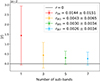 |
Fig. B.1. Mean and standard deviation of the best-fit distributions obtained with Commander, using the d6s1 model with ℓcorr = 10 and r = 0. |
Increasing the number of sub-bands also reduces the standard deviation of the marginalized posterior distributions of the standard deviation of the spectral indices for all pixels. Figure B.2 shows the comparison between the reconstructed dust and synchrotron spectral indices. As in Appendix A, we compared reconstructed spectral indices with the input ones, from Planck Collaboration X (2016) for one, three, and five sub-bands on all pixels. Because of frequency de-correlation, the spectral indices residuals for dust are not as meaningful as the distribution of reconstructed r shown in Fig. B.1. This analysis has not been performed for the seven sub-band configuration results because of data storage issues. Here a single Δβ from the plotted distributions represents the difference between the mean value of the marginal distribution on a single pixel for a given sky realization and the template value in the same pixel from the model. These results are in agreement with the FGBuster simulations.
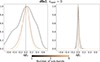 |
Fig. B.2. Reconstruction of foreground spectral indices for the d6s1 model with the Commander pipeline. |
All Tables
All Figures
|
Fig. 1. Schematic of the QUBIC instrument, showing the principle of BI. The sky signal is received by an array of back-to-back horns and reimaged onto the bolometric focal planes, where the field interferes additively. A polarizer and a rotating half-wave plate make the instrument sensitive to linear polarization. |
| In the text | |
|
Fig. 2. Synthetized beam of QUBIC. Top panel: simulation of the interference pattern on the focal plane generated by a monochromatic point source. Bottom panel: azimuth cut of the theoretical synthesized beam (solid lines) at 140 GHz (blue line) and at 160 GHz (green line) for a detector at the center of the focal plane. Dashed lines represent the beam pattern of a single feed horn. The frequency-dependent position of the secondary peaks is clearly visible. |
| In the text | |
|
Fig. 3. Dispersion of the dust SED for different correlation lengths of the PySM d6 model normalized by the single MBB emission (d1 model). The colored areas represent the statistical deviation from a MBB for a given correlation length, evaluated over 500 realizations. |
| In the text | |
|
Fig. 4. Correlation ratio measured by Planck from the Half Mission (HM) maps at 217 GHz and 353 GHz, compared to the simulated ratio using PySM dust and CMB templates at the same frequencies. The blue and orange dots represent the expected Rℓ for the CMB and a single MBB dust emission, with constant (d0) or varying pixel-by-pixel (d1) spectral indices, respectively. Note that the dots are so close that they overlap in the figure. The green envelope shows the range of Rℓ obtained from 500 realizations of dust LOS frequency de-correlation with ℓcorr = 10. The black dots are from Fig. 2 of Planck Collaboration Int. L (2017), the gray dots are from Fig. B.2 of Planck Collaboration XI (2020), and the red point is obtained from the values in the middle plot of the second row in Fig. 18 of Planck Collaboration XI (2020). |
| In the text | |
|
Fig. 5. Polarization sensitivity of CMB-S4 and three examples of CMB-S4/BI, with nsub = 3, 5, and 7, respectively. Note that the bands of the three lowest-frequency channels are identical for all the instruments. Because our study focuses on dust de-correlation, we chose not to split the bandwidths of the synchrotron channels. |
| In the text | |
|
Fig. 6. Normalized histograms of the maximum likelihood values of r as a function of the number of sub-bands. Top left: model d0s0 with rinput = 0. Top right: model d1s1 with rinput = 0. Bottom left: model d1s1 with rinput = 0.006. Bottom right: model d6s1 with ℓcorr = 10 and rinput = 0. |
| In the text | |
|
Fig. 7. Average maximum likelihood value of r and the standard deviation as a function of the number of sub-bands in the case of unaccounted-for dust frequency de-correlation (model d6s1 with ℓcorr = 10 and r = 0) compared to two cases of no de-correlation (model d1s1): r = 0 and r = 0.006. On top of the average r values and their standard deviation, we have overplotted the shape of the distribution as a “violin plot.” Note that for the d6 case the distribution is asymmetric for small nsub, so that the average is not centered on the distribution. |
| In the text | |
|
Fig. 8. Summary of the average maximum likelihood value of r and the standard deviation for an input r = 0 and all the simulated foreground models (d0s0, d1s1, and several ℓcorr cases of d6s1). Note that we assume symmetric error bars. |
| In the text | |
|
Fig. 9. Confusion matrix representing our ability to classify between our simulated datasets with dust frequency de-correlation (contaminated) or without (clean) using the measurements of r as a function of nsub. We observe that the fraction of false negatives (contaminated dataset incorrectly classified as clean) is close to zero. |
| In the text | |
|
Fig. A.1. Reconstruction of foregrounds spectral indices. Top: Model d0s0, rinput = 0. Middle: Model d1s1, rinput = 0. Bottom: Model d6s1, rinput = 0. |
| In the text | |
|
Fig. B.1. Mean and standard deviation of the best-fit distributions obtained with Commander, using the d6s1 model with ℓcorr = 10 and r = 0. |
| In the text | |
|
Fig. B.2. Reconstruction of foreground spectral indices for the d6s1 model with the Commander pipeline. |
| In the text | |
Current usage metrics show cumulative count of Article Views (full-text article views including HTML views, PDF and ePub downloads, according to the available data) and Abstracts Views on Vision4Press platform.
Data correspond to usage on the plateform after 2015. The current usage metrics is available 48-96 hours after online publication and is updated daily on week days.
Initial download of the metrics may take a while.