| Issue |
A&A
Volume 684, April 2024
|
|
|---|---|---|
| Article Number | A80 | |
| Number of page(s) | 20 | |
| Section | Planets and planetary systems | |
| DOI | https://doi.org/10.1051/0004-6361/202347813 | |
| Published online | 05 April 2024 | |
Quantitative grain size estimation on airless bodies from the negative polarization branch
I. Insights from experiments and lunar observations★
1
Korea Astronomy and Space Science Institute (KASI),
776 Daedeok-daero, Yuseong-gu,
Daejeon
34055, Republic of Korea
e-mail: ysbach93@gmail.com
2
Department of Physics and Astronomy, Seoul National University,
Gwanak-ro 1, Gwanak-gu,
Seoul
08826, Republic of Korea
3
SNU Astronomy Research Center, Department of Physics and Astronomy, Seoul National University,
Gwanak-ro 1, Gwanak-gu,
Seoul
08826, Republic of Korea
e-mail: ishiguro@snu.ac.kr
4
Center for Astronomy, University of Hyogo,
407-2 Nishigaichi, Sayo,
Hyogo
679-5313, Japan
5
Japan Spaceguard Association,
Bisei Spaceguard Center 1716-3 Okura, Bisei, Ibara,
Okayama
714-1411, Japan
6
Nayoro Observatory,
157-1 Nisshin, Nayoro,
Hokkaido
096-0066, Japan
7
Department of Astronomy, Graduate School of Science, The University of Tokyo,
7-3-1 Hongo, Bunkyo-ku,
Tokyo
113-0033, Japan
Received:
28
August
2023
Accepted:
8
January
2024
This work explores characteristics of the negative polarization branch (NPB), which occurs in scattered light from rough surfaces, with particular focus on the effects of fine particles. Factors such as albedo, compression, roughness, and the refractive index are considered to determine their influence on the NPB. This study compiles experimental data and lunar observations to derive insights from a wide array of literature. Employing our proposed methodology, we estimate the representative grain sizes on the lunar surface to be D ~ 1–2 µm, with D ≲ 2–4 µm, consistent with observed grain size frequency distributions in laboratory settings for lunar fines. Considering Mars, we propose that the finest particles are likely lacking (D ≫ 10 µm), which matches previous estimations. This study highlights the potential of multiwavelength, particularly near-infrared, polarimetry for precisely gauging small particles on airless celestial bodies. The conclusions provided here extend to cross-validation with grain sizes derived from thermal modeling, asteroid taxonomic classification, and regolith evolution studies.
Key words: minor planets, asteroids: general / minor planets, asteroids: individual: (1) Ceres / minor planets, asteroids: individual: (4) Vesta
Part of the codes and data used for this publication are available via GitHub: https://github.com/ysBach/BachYP_etal_CeresVesta_NHAO.
© The Authors 2024
 Open Access article, published by EDP Sciences, under the terms of the Creative Commons Attribution License (https://creativecommons.org/licenses/by/4.0), which permits unrestricted use, distribution, and reproduction in any medium, provided the original work is properly cited.
This article is published in open access under the Subscribe to Open model. Subscribe to A&A to support open access publication.
1 Introduction
With current aspirations for space exploration, numerous airless objects have been thoroughly investigated and leverage advanced scientific approaches, such as orbiters, flybys, and landers. These explorations have facilitated the study of the geology, shape, dynamics, and consequences of impacts on these celestial remnants (e.g., the recent DART mission by Daly et al. 2023). Despite extensive exploration, direct visual observation of decamicron-scale dust particles has not been performed since few images have been able to resolve such fine scales on the surface. However, the presence of these fine particles can impact scattering or emission processes, thereby modulating the observed light. As a result, indirect methods, such as thermal modeling (Gundlach & Blum 2013; MacLennan & Emery 2022b) and polarimetric observations (Geake & Dollfus 1986; Ishiguro et al. 2017; Ito et al. 2018; Bach et al. 2019), have been employed to explore the existence of these fine particles. We focus on the latter approach and suggest a novel way to estimate grain sizes using multiwavelength polarimetry.
In reality, any solid surface is composed of an irregular spatial distribution of dielectric coefficients, that is, has a degree of disorder, which is often practically impossible to describe mathematically. Thus, as a rough approximation, the disorder is described by using familiar terms, such as grain size, reflectance/albedo, composition, surface roughness, and macro/microporosity.
Typically, in Fresnel reflection or Rayleigh scattering, the strongest electric field vector aligns perpendicularly to the scattering plane (the plane formed by the incident and emitted light rays). However, at small phase angles, the strongest electric vector is predominantly parallel to the scattering plane for rough surfaces (the first report was by Brewster 1863). Recognizing this behavior, Lyot (1929) proposed a modified linear polarization degree for use in observational and experimental studies:

where P represents the total linear polarization degree, θr is the position angle of the strongest electric vector relative to the normal vector of the scattering plane (0/180°: normal to the scattering plane, 90/270°: within the scattering plane), and I⊥ and I|| denote the measured intensities of scattered light along the directions perpendicular and parallel to the scattering plane, respectively.
The polarimetric phase curve (PPC), represented by Pr(α), is plotted as a function of the phase angle (light source-target-observer angle; α : = 180° – scattering angle) and exhibits a distinctive pattern. This curve, which is studied extensively in previous research (e.g., Geake & Dollfus 1986, and references therein), can be divided into different regions. Near the opposition (α = 0), Pr < 0, where it reaches the minimum Pr(α = αmin) = Pmin < 0 at αmin ≲ 10°. Then, Pr becomes positive after the inversion angle (α0 ~ 15–30°) and reaches the maximum Pr(α = αmax) = Pmax at αmax ~ 90–150°. Consequently, the region with α < α0, where Pr < 0, is referred to as the negative polarization branch (NPB), while the α > α0 region is known as the positive polarization branch (PPB).
PPC has been extensively studied since the pioneering works of Lyot (1929) and Dollfus (1955). Several physical explanations for the NPB have been proposed, most notably the coherent backscattering mechanism (Shkuratov et al. 1994; Muinonen et al. 2002; Belskaya et al. 2015; Hapke 2012, and references therein). Empirically, it has been shown that the NPB is influenced by factors such as particle size (Geake & Geake 1990), albedo contrast and/or mixing (Shkuratov 1987; Spadaccia et al. 2022), multiple reflections of absorbing particles (Dollfus 1956; Dollfus et al. 1971b), and specifically, double reflections along the side-way direction (Wolff 1975, 1980, 1981, Geake et al. 1984; Fig. 13.17 in Hapke 2012), as well as large-scale surface roughness and/or compaction (Geake et al. 1970; Shkuratov et al. 2002; Appendix of Spadaccia et al. 2022). Many theoretical improvements have proposed that the real part of the refractive index and interparticle distance at given wavelengths, as well as the particle size distribution, are important parameters (Muinonen et al. 2002a; Masiero et al. 2009). Among these factors, the effect of particle size can be used to indirectly measure particle size and complement other size estimation methods, such as thermal modeling.
Moreover, after qualitative discovery by Umow (1905), the tendency toward stronger polarization for lower albedo is called the Umov law or the Umov effect (e.g., Hapke 2012, Sect. 13.3.2). However, the albedo-Pmax relation varies based on several physical factors, notably particle size (Geake & Dollfus 1986; Dollfus & Deschamps 1986; Dollfus et al. 1993). Another important relation between the albedo and polarimetric slope (h : = dPr/dα(α = α0); first noted in Widorn 1967) seems to follow a tight relation regardless of the object (Veverka & Noland 1973; Bowell et al. 1973; Geake & Dollfus 1986; Cellino et al. 2015; Lupishko 2018, to name few). There is another correlation between albedo and Pmin (e.g., Cellino et al. 2015; Lupishko 2018). For simplicity, we refer to both the h-albedo and Pmin-albedo relations as Umov law(s) in this paper. Specifically, the former is colloquially called the “slope-albedo law”, a name that has likely been used since Bowell et al. (1973). These relations have been widely used to estimate the albedo of asteroids from polarimetric observations (Lupishko 2018; Ishiguro et al. 2022; Geem et al. 2022, 2023).
In this study, we focus on investigating the NPB through an empirical approach. We emphasize that the experimental data are scattered across diverse literature sources, with variations in the definitions of albedo, polarimetric parameters, sample preparation methods, and experimental conditions. While compiling the sources, we recognized typos and errors in the figures and tables sourced from cross-referenced literature. Additionally, several crucial trends identified in this work received limited coverage in the original literature. As a result, our initial efforts were concentrated on investigating, collecting, and consolidating the published experimental datasets and extracting a trend that is practically useful for grain size estimation.
We compiled existing experimental data from published sources and excluded results from theoretical studies. We limited our focus to (i) the NPB of linear polarization (ii) under unpolarized incident light by (iii) a thick powdery surface of (iv) solid non-icy, non-metallic surface samples with (v) reasonable accuracy. For accuracy, as a rule of thumb, we used ΔPmin ≲ 0.3 %p, Δα0 ≲ 2°, etc., as criteria, depending on the shape of the PPCs. Icy surfaces are an important subject of study, especially for outer solar system objects. However, it is challenging to keep them frozen without sintering during the measurements, and the PPC depends on the regolith property below the ice (Dougherty & Geake 1994; Spadaccia et al. 2023), which complicates the interpretation. Despite their transparency, glass powder samples are discussed multiple times due to the wealth of available experimental results.
We also did not extensively explore the polarization opposition effect (POE), which is believed to arise from the coherent backscattering phenomenon (Shkuratov 1989; Muinonen 1990; Sect. 13.4 of Hapke 2012). The POE was reported as early as Lyot (1929) for a MgO coating, leading to the identification of a distinct sharp negative polarization peak at very small α (~1°). This effect significantly contributes to the asymmetry of the NPB. While it is possible to explore the POE by introducing skewness-related parameters, we opted not to do so due to the limited availability of samples with skewness information. This limitation stems from the fact that the original publications either could not reliably measure the full PPC at small phase angles due to experimental constraints or reported only Pmin without presenting the complete PPC. We only qualitatively described POE when necessary.
We first describe the data we collected (Sect. 2). Then, using these data, we revisit the Umov laws (h–albedo and Pmin–albedo; Sect. 3), including lunar and asteroid observations, to obtain the first ideas of the correlations. Next, we discuss the effect of fine particles a few times larger than the observation wavelength (Sect. 4). Afterward, we disentangle the possible effects of albedo, compression, and the refractive index (Sect. 5). Equipped with this, we try to quantify the effect of fine particles, now down to the subwavelength scale (Sect. 6). The essence of the methodology is summarized in Sect. 7 (Fig. 10). Afterward, we justified our strategy developed throughout this work by estimating the grain sizes of selected celestial objects (Sect. 8). Finally, we briefly discuss how this work complements an independent thermal modeling approach (Sect. 8.4) and provide a future perspective (Sect. 9).
We also present our observational data for (1) Ceres and (4) Vesta in multiple figures, as well as optical data from published resources. However, detailed discussions of these airless objects are provided in the companion paper (Bach et al. 2024; hereafter Paper II). Thus, we do not discuss them in this work, although they are shown in the figures.
2 Experimental data
There has been an enormous amount of effort put into experimental studies to understand the PPC of celestial objects. Levasseur-Regourd et al. (2015) provides a thorough review of multiple instruments and results, especially for PROGRA2 [-Surf] (Worms et al. 2000; Hadamcik et al. 2009). Table 1 summarizes the samples and original publications that are most relied on in this work. The collected datasets are briefly described in Sect. 2.1. Due to the importance of the alumina experiment (Geake & Geake 1990; GG90 hereafter), this experiment is described in detail in Sect. 2.2, and the refractive index of alumina is discussed in Sect. 2.3 for use in later parts of the study.
Sources of experimental data.
2.1 Description of compiled data
Different publications used different definitions of albedo, making direct data comparison challenging. The two most widely used methods are denoted MgO5 (albedo measured at α = 5° with respect to a thick MgO-smoked plate) and H2 (α = 2° with respect to compressed Halon). For the former, MgO5-N indicates that the publication explicitly mentioned the use of normal incidence when illuminating the MgO plate. Similarly, the definition of slope h has at least two widely used definitions: linear regression to α ∈ [α0, α0 + 10°] and fitting a second-order polynomial (“parabola”) for data at α ∈ [α0 − 5°, α0 + 10°]. We call the former the 0–10–1 slope and the latter the 5–10–2 slope. We note that the exact definition of h changes its value significantly for some PPCs.
We primarily used Geake & Dollfus (1986) as the main reference. These authors included measurements made only at the “orange” filter (λ = 5800 Å, half-width ~500 Å). The tables provide tabulated values based on the Meudon Observatory log book. We call their tabulated data T0. In T0, the PPCs were measured at the specular geometry, and the albedos are the MgO5-N albedos. The uncertainties are ΔPmin = 0.05 %p, ΔPmax = 0.1 %p, ΔA = 0.01, and Δh = 0.005%/°, but the uncertainties for each sample were not provided. The slope h values in T0 are in the 0–10–1 scheme.
Given that the table (T0) and figures in Geake & Dollfus (1986) do not match for some samples (Bach et al. 2019), we relied on the values provided in T0, not the figures. We carefully cross-checked the numeric values in T0 against those from the original references. If the differences were negligible (roughly the size of the markers in the figures shown in this work), we prioritized the values presented in T0. If the differences were nonnegligible, we treated them as separate samples.
More lunar or terrestrial sample data (including volcanic ash) from Dollfus & Geake (1975) and Zellner et al. (1977a) are included. Terrestrial samples from the latter are explicitly described as <25 µm, so we labeled them “Terr. (< 25 µm)”, even though T0 used the notation “smaller than 50 µm”.
Many terrestrial samples were obtained from Lyot (1929), especially from Table 15. Since they do not describe whether they removed dust from the rocks, we carefully cross-matched samples in this and T0 samples, separated them from the dustfree sample, and labeled them simply “Terr. rocks”. These results are likely comparable to those of the “lunar dusty rock” samples. Transparent crystal samples (e.g., NaCl) and three mineral powder samples (magnetite, pyrite, and galena) are collectively labeled “Lyot’s powder”. The study also included powdered lava samples which were reported to exhibit size D = 100–200 µm. The “Volcanic ash” samples included a wide range of grain sizes.
The PPCs and Table 15 of Lyot (1929) are carefully compared with the values reported in T0. We found and fixed a few typos and mismatches. For mismatches, we prioritized the PPC: The value that better matches the PPC was adopted. When both of the tabulated values were clearly different from the PPC (e.g., Pmax is reported from hand-drawn curves, not from the real data points, and they differ greatly), we fixed it by visual inspection of the actual data points. Although the definition of albedo reported is not clear1, we assumed it was a MgO5 scheme under λ = 0.580 µm (see Geake & Dollfus 1986).
All the crushed meteorite samples from Zellner et al. (1977a) are included. The authors generated “crushed but not ground or sieved” meteorite samples to simulate cratering on asteroids, and the resulting grain sizes were reported to be ≲500 µm. We marked these samples as “Meteo. Powder” for simplicity because the exact grain sizes are unavailable. The volcanic ash data (with only qualitative sample descriptions) are also adopted. The slope h values are measured under the 5–10–2 scheme.
Le Bertre & Zellner (1980) contain PPCs and/or verbal explanations of eucrites (Moama, Bereba, “Bereba B” mixture, and Padvarninkai mixture) but lacks quantitative values for polarimetric parameters. Thus, based on the data presented in the figures or text, we extracted h, αmin, α0, and Pmin information, but albedo information was unavailable in most cases.
Lupishko & Belskaya (1989) contains 13 meteoritic, five terrestrial, and five metal samples, with grain sizes of ≤50 µm. The authors used the MgO5-N albedo scheme for the freshly deposited MgO plate.
Shkuratov et al. (1984) reported PPCs of pulverized (size D < 100 µm) and cleaved faces of Allende and Kainsaz. We recovered polarimetric parameters by visual inspection. The albedos are measured at α = 3° and λ = 0.56 µm. The authors described that the cleavage face “do not exhibit either the slightest trace of any dust coat or any evidence of complex microrelief”. Thus, we included cleavage samples in the “Dust-free” category.
Zellner et al. (1977b) provided valuable data for artificial silicates, described “nearly amorphous hydrated magnesian silicate, MgO • SiO2 • H2O”, with added carbon and/or black paint. We have included all their data (Pmin, 5–10–2 slope h, MgO5-N albedo, α0). We also added αmin by visual inspection. Carbon particles are reported to have a size of 0.01 µm, but no information is given for silicate. Considering the description in Dollfus & Zellner (1979), which reports that, “The powders made of pulverized silicates … are strongly depleted in micron-size grains when compared to the lunar soil”, we expect the particle sizes for the silicate powder to be much larger than those of the carbon particles (especially compared to 10 µm silica in Spadaccia et al. 2022).
The two “candle soot” datasets of the MgO5-N albedo (1.1%) are adopted from Zellner et al. (1977a). These are described as “deposited on tray” and “loosely piled”. Another soot (rubber soot) dataset with a H2 albedo of 2.6% is obtained by fitting to the PPC in Shkuratov et al. (2002); this sample is prepared by incinerating black rubber and particle sizes D ≪ 1 µm.
Shkuratov et al. (1992) show the transparent glass powder and soot-MgO mixtures. Since we could not access the quantitative albedo and grain size information, only Pmin-α0 information was reconstructed. Similarly, we extracted as much information as possible from Shkuratov et al. (2002) and included other glass powders in this work, combining them into “transparent glass powder”. The albedo information is available only as “moderate albedo, 40–60%”. Figure 23 of Shkuratov et al. (1994) shows black, green, and clear glass powders in the log10(D)-Pmin and log10(D)–α0 spaces. Among them, we recovered the (Pmin, α0) pair only for the clear glass samples because the number of samples in the two panels differs for the other glass samples.
Shkuratov (1987) reported the PPCs of glass, soot, MgO, and Fe2O3 fine powder (size D < 1 µm) and their mixtures. They argued that the NPB develops when the contrast in albedo between the endmembers increases. The PPCs of Fe2O3 and soot are different from those of Shkuratov et al. (2002) and Belskaya et al. (2005), respectively, which is likely because of the different samples and preparation steps. We did not include the samples presented in this work but qualitatively describe them when necessary.
Shkuratov et al. (2004) provided some valuable experimental data for fine samples (with sizes ranging from D = 2–14 µm). We calculated Pmin, α0, αmin, and h by visual inspection, and we noted the possibility of greater uncertainty. The figures for feldspar and loess are identical in the publication, likely by mistake, although albedos seem to be correctly written in the figures. Based on the slope-albedo law, we concluded that the figure for the loess mistakenly overlie the feldspar one. The blue-wavelength PPC corresponding to feldspar could be restored from Fig. 14 in Shkuratov et al. (2006). Although Shkuratov et al. (2007) show the full results for feldspar, the NPBs are printed at low resolution, and possibly because of this, some α0 values do not coincide with the previous values for the same sample. Their albedos are in the H2 scheme (Shkuratov et al. 2004).
Shkuratov et al. (1992) and Belskaya et al. (2005) report soot and MgO mixture results. The former shows multiple samples with Pmin and α0, while the latter provides two PPCs of pure soot (albedo 3.4%) and a soot+MgO(5% wt) mixture (albedo 4.3%). The definition of albedos is not given, but it is likely the H2 scheme.
Spadaccia et al. (2022) conducted a significant study on the mixing effect of minerals. In their work, the illuminated region on the sample was approximately 15 mm in diameter under λ = 0.53 µm, and the “albedo” adopted in this work was hemispherical-directional reflectance. All the powder samples had grain sizes D < 20 µm, although silica formed larger aggregates. Their SEM images show that the grain sizes are comparable to the wavelength scales, especially for the forsterite and magnetite samples. Given the important information provided by of their samples and high-quality data, we have collected their PPCs2 and obtained the corresponding NPB parameters, including the 5–10–2 scheme h values. Each of the fitted curves was visually inspected, and our α0 values matched well with the reported values within the error bars; therefore, we adopted α0 from the publication. We carefully compared the available PPC and the published values and corrected two typos (α0).
Sultana et al. (2023) reported a series of hyperfine particle experiments in which Mg-rich (forsterite) olivine was used D = 0.6 µm and iron sulfide (FeS) was used D = 0.2 µm (see their Table 1 and supplementary Fig. 3). Polarimetry was conducted under the normal emission geometry at λ = 0.53 µm, and the albedo is the solar spectrum-averaged “equivalent” albedo estimated from λ = 0.56 µm reflectance3 (Beck et al. 2021). After collecting their PPCs, we calculated the NPB parameters, especially the 5–10–2 h and α0 values, as above.
2.2 Description of the alumina experiment (GG90)
In this work, and its underlying logic, the alumina sample data (GG90) play a pivotal role. We collected Pmin, α0, and MgO-5 albedo values, if available, from the publication. Their measurements were conducted using four filters attached to a Minipol mounted on a B. H. Zellner’s goniometer, denoted as B (blue), G (green), R (red), and I (infrared), corresponding to peak wavelengths of λ = 0.440, 0.535, 0.685, 0.790 µm, respectively. These filters were applied in conjunction with various particle sizes (D = 40, 12, 3, 1, 0.3, 0.05 µm), resulting in a total of nine distinct D/λ measurements spanning the range from 0.093 to 75. The samples were on a blackened stainless steel, 4 mm depth, “pressed flat with a spatula”, observed at the specular geometry, rotated by motor to “average out the effects of any specular reflections from grain facets”, so that D/λ is the only parameter changing over various measurements.
Notably, among these measurements, those for D/λ = 75, 22, 5.6, 1.9, 0.56, and 0.093 were conducted with the same G filter. This unique set of measurements provides an opportunity to isolate the effects of the refractive index and grain size. Additionally, for D/λ = 75, 0.56, and 0.093, carbon particles (D = 0.01 µm) were added to alter the albedo of the samples, with all the measurements conducted within the G filter.
Their results are summarized in the Pmin-α0 space in Fig. 1. The authors found the following trend in the NPB as the wavelength (λ) increased:
Unchanged when D/λ ≫ 5 (samples of D/λ = 22, 75).
Wider and deeper (WD, hereafter) when D/λ ~ 5 → 2.
Narrower and deeper (ND, hereafter) when D/λ ≲ 2.
In their study, Pmin values for samples with D/λ = 0.093 are estimated through extrapolation; thus, we consider these values to be uncertain. Furthermore, their PPCs exhibit a notably sharp NPB at small α when D/λ ≲ 1, which is indicative of a strong POE, even for these flattened samples. While it would be ideal to treat the broad NPB and the POE separately, for the purposes of this work, we simply use Pmin and α0 in our analysis. These findings suggest that the ND trend may be closely associated with the POE and coherent scattering characteristics (Shkuratov 1989; Muinonen 1990; Sect. 13.4 of Hapke 2012).
Because h values were not provided in GG90, we digitized the PPC values for α < 40°. Because of the limited number of data points, we could not calculate h under the 0–10–1 or 5–10–2 schemes. Rather, we fit a linear line to the six data points nearest to α0. This approach was further validated by ensuring that the α0 derived from this linear fit remained consistent with the original values reported in the publication.
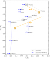 |
Fig. 1 Laboratory samples in Pmin-α0 (depth-width of NPB) space. The numbers to the right of the alumina indicate D/λ and the filter, while the blue numbers to the left (with unit %) are the albedo values. D/λ = 0.093 data points are enclosed in parentheses because their Pmin values are extrapolated values. The WD and ND trends, with increasing λ (or decrease D/λ), are schematically indicated. |
2.3 Refractive index of alumina
The refractive index n = n(λ) is known to affect the NPB (Muinonen et al. 2002b). Consequently, for future discussion, we have compiled information on n(λ) for alumina (aluminum oxide, Al2O3, also called [synthetic] sapphire in the literature) reported in various sources.
2.3.1 Wavelength dependence
One of the first reported values under ordinary rays was tabulated in Malitson (1962), and a dispersion relation was proposed to be established at 24 °C for λ = 0.26–5.5 µm (λ in µm):

The selected measurements are:

At an annual meeting of the Optical Society of America, an updated version was presented (Malitson & Dodge 1972). At 20 °C, for λ = 0.20–5.0 µm (recited from TABLE II of Tropf & Thomas 1997 and Sect. 1.3.4 of Weber 2002):

for the ordinary and extraordinary rays, respectively. At selected wavelengths, the calculated values are:

A later report by Querry (1985) tabulated the n(λ) value for polarizations parallel (n||) and perpendicular (n⊥) to the crystal c-axis. The values at the two selected wavelengths are:

We note that these values deviate largely from those of other works.
Tropf & Thomas (1997) reported n(λ) for ordinary (no) and extraordinary (ne) rays. Selection from their work:

Combining these (except inconsistent values from Querry 1985), the refractive index of alumina is decreased by ~0.02 from B (0.44 µm) to I (0.79 µm) filter used in GG90, as shown in Fig. 2.
2.3.2 Temperature dependence
In regard to the temperature dependence of the refractive index,  and Vedam et al. (1975) reported that, under the “room temperature (RT)”,
![$\left( {{n_{To}},\,{n_{Te}}} \right)\,({\rm{RT}},0.589\,{\rm{\mu m}}) = (13.6,\,14.7) \times {10^{ - 6}}\,\left[ {{{\rm{K}}^{ - 1}}} \right]$](/articles/aa/full_html/2024/04/aa47813-23/aa47813-23-eq9.png)
for ordinary and extraordinary rays, respectively.
Dodge (1986; recited from Weber 2002 Sect. 1.3.5) reported that, at λ = 0.4579 µm:
![$\matrix{ {\left( {{n_{To}},{n_{Te}}} \right)\left( { - {{180}^ \circ }{\rm{C}},\,0.4579\,{\rm{\mu m}}} \right) = (1.8,1.9) \times {{10}^{ - 6}}\,\left[ {{{\rm{K}}^{ - 1}}} \right],} \hfill \cr {\,\,\,\,\,\,\,\,\,\left( {{n_{To}},{n_{Te}}} \right)\left( {{{20}^ \circ }{\rm{C}},\,0.4579\,{\rm{\mu m}}} \right) = (11.7,12.8) \times {{10}^{ - 6}}{\kern 1pt} \,\left[ {{{\rm{K}}^{ - 1}}} \right],} \hfill \cr {\left( {{n_{To}},{n_{Te}}} \right)\left( {{{200}^ \circ }{\rm{C}},\,0.4579\,{\rm{\mu m}}} \right) = (15.4,16.9) \times {{10}^{ - 6}}\,\left[ {{{\rm{K}}^{ - 1}}} \right].} \hfill \cr } $](/articles/aa/full_html/2024/04/aa47813-23/aa47813-23-eq10.png)
Tapping & Reilly (1986) reported a fitting formula for the ordinary ray under T = 24−1060 °C (to the 0.02% with 99% confidence level):

where the temperature T is °C.
Therefore, for a main-belt asteroid with a diurnal temperature variation on the order of ΔT = 102 K, the expected change (nT) is on the order of 10−3 throughout the wavelength range of interest. For the related alumina experiment, the wavelength-dependent change is already an order of magnitude larger than that related to temperature, and ΔT in the experiments must be very small, such that nT can be neglected in our analyses.
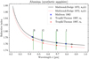 |
Fig. 2 Refractive indices of alumina (Al2O3) from various sources (see text for details). Available measurements closest to the central wavelengths of the filter (B, G, R, and I used in GG90) are indicated with markers. |
3 A first look: The Umov laws (albedo-h-Pmin)
3.1 The correlations
Among the Umov laws, the slope-albedo relation is well known for its tightness. In Fig. 3, we plot the compiled samples in the h-albedo space. The overturn of the linear relation, as evidenced by candle soot and silicate-carbon mixtures, starts to appear at albedo ≲5%. Zellner et al. (1977b) explained this with the extremely reduced amount of double scattering by dark inclusions, based on Wolff (1975). This trend has also been found for asteroids (Cellino et al. 2015). Figure 4 in Shkuratov et al. (1992) also shows the overturning at low albedo for water-color samples. For high-albedo objects, the h-albedo correlation appears to become less distinct.
The Pmin-albedo relation, shown in Fig. 4, is known to be more scattered than the slope-albedo law (e.g., Dollfus & Zellner 1979 for experiments and Cellino et al. 2015 and Lupishko 2018 for asteroid observations). One logical hypothesis is that there is a strong secondary parameter that controls this Pmin-albedo relation, such as particle size, compaction, and roughness. Like in the slope-albedo relation, Pmin-albedo relation also shows an overturn or departure from the general trend in the lowest and highest albedo regions.
The general asteroid trend in the figures (blue solid lines from Lupishko 2018) shows the geometric albedo. Thus, asteroid “albedo” values must be systematically larger than those of laboratory samples due to the opposition surge. Additionally, the albedo of lunar observation (Shkuratov et al. 1992) is measured at α = 3.1°, while assuming that αmin = 10.5°, that is, Pmin = Pr(α = 10.5°). By comparing the tables and figures for the lunar observation, we found some mismatches; therefore, we consider the table values; because mare craters and highland craters are oppositely labeled, we correct for this.
The two-band lunar observations in Fig. 3 show a small systematic shift in the trend for the two wavelengths. In red, h is larger (steeper) than expected at the same albedo in blue. The lunar data in Fig. 4 exhibit a behavior that diverges from the typical trend observed for asteroids. The trend even appears to run in the opposite direction in the case of maria.
Figure 5 shows identical relationships but for the mineral and silica mixture samples. Their albedos are defined differently from those in Figs. 3 and 4, so they cannot be compared directly. Olivine samples and mixtures (ol, fo, fa) lie on a smooth curve, even though they are from two independent studies, strengthening the credibility of the experiments.
3.2 Samples worth noting
The distribution of alumina in D/λ < 2 is largely different from that in the other D/λ > 5 samples in both parameter spaces. GG90 noted that each group of samples with D/λ = 75, 0.56 and 0.093 qualitatively follow the Umov law in the Pmin-albedo space: higher albedo samples have shallower Pmin (they did not describe slope h). The transparent glass powder samples in Fig. 4 also show a deepening trend as the grain size decreases to the scale of λ, similar to alumina. Additionally, although not plotted, D < 1 µm glass powder samples of 67% and 89% H2 albedos (Shkuratov 1987) are located near alumina samples of D/λ = 0.56 or 1.9 in both parameter spaces.
There are two outliers among high albedo terrestrial rock samples in Fig. 4: The chalk4 and the white clay5. The original report (Lyot 1929) mentioned that chalk has a similar PPB shape to that of precipitated chalk6. For the white clay, the report described it is “somewhat remarkable” to show such a deep NPB for its albedo, though no further description is given. The NPB shape of the white clay (sharp minimum at αmin = 3°) is similar to that of small alumina samples (GG90), which hints at the possibility of the existence of fine particles.
Among “Lyot’s powder” samples, the magnesia coating7 is worth attention. The original report noted that the sharp Pmin at a very small αmin is attributed to the fine particle size of the sample. A micrograph of the MgO coating showed a similar PPC (Fig. 3 of Shkuratov et al. 2002) and indeed confirmed the presence of a plethora of subλ particles in the sample. Notably, the MgO samples from both works are located near the alumina sample of D/λ < 1.
As shown in Fig. 5, the spi-graph mixture has a smaller h and shallower NPB than the other samples with similar albedos. However, ol-FeS mixtures reach higher h and deeper NPB than other samples of similar albedo, which may be linked to their specific fine, subλ scale grain sizes. For very fine samples (D < λ), the α0 and |Pmin| of mixtures are greater than those of both endmembers (Shkuratov 1987). Interestingly, both h and Pmin change greatly when albedo is fixed for the fo-spi mix, similar to glass powder (Fig. 4). Generally, the mixtures continuously change between the endmembers. Other samples also roughly follow the typical trends expected by the Umov law.
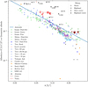 |
Fig. 3 Slope (h)-albedo relation. See Sect. 2 and Table 1 for the details of the laboratory data and their original sources. The numbers next to the alumina samples are the D/λ values. The telescopic lunar observation data from Shkuratov et al. (1992) are shown for blue (0.42 µm) and red (0.65 µm) wavelengths using cyan and magenta colors, respectively, and the same regions are connected by a thin line. The lunar albedo is defined at α = 3.1°, so it should be smaller than the geometric albedo. The blue solid line is the regression line for asteroids (Lupishko 2018). The Ceres and Vesta results are shown as red and dark red, respectively, and are connected in the order of increasing wavelength: υ = 0.45–0.60 µm, r = 0.60–0.75 µm, i = 0.75−1.0 µm, J-, H-, and K-bands (Paper II). |
4 Grain size (D/λ) effect: The widening and deepening (WD) trend
The size parameter X : = πD/λ is a controlling parameter for scattering processes once the refractive index is known (Bohren & Huffman 1983). For an observer, the target object has a fixed D, so changing λ leads to an adjustment of X; thus, the scattering process will be affected. To easily compare with the experimental studies (especially GG90), we use D/λ (= X/π), rather than X.
Pmin and α0 describe the shape of the NPB in the first order (in terms of depth and width, respectively). In Fig. 6, we plotted the compiled samples and lunar observations in the parameter space. As proposed previously, particle size indeed changes NPB-related parameters: fine particle samples are well separated from other dust-free rock samples. Smaller particle samples generally show a wider and often deeper NPB (Dollfus & Geake 1977). Dollfus et al. (1989) used this diagram to argue that asteroids are covered with coarser particles than on the Moon.
Below, we further discuss the evidence supporting the WD trend, including the widening and deepening trend with decreasing D/λ, based on previous experimental works and lunar observations. Then, we attempt to quantify at which D/λ the WD trend starts to occur.
4.1 Previous works
Figure 12 in Dollfus (1961) shows the WD trend for iron filings as the particle size decreases. Figure 1 of Dollfus et al. (1969) shows widening (but no clear deepening) as the wavelength increases in the case of pulverized limonite. In a study by Kenknight et al. (1967), changes in the NPB according to laboratory experiments were observed, with a deepening effect as λ increased. However, further discussion was limited, which is potentially attributed to crude particle size segregation. Later, GG90 conducted alumina powder experiments under varying D/λ conditions (Sect. 2.2).
Shkuratov et al. (1992) briefly mentioned that they observed a qualitatively similar WD trend for transparent glass powders of size D = 0.5–200 µm (Figs. 3 and 4, and in Fig. 6). In addition, this same WD trend (likely correlated with D/λ) is clearly observed for the green, clear, and black glass samples in Fig. 23 of Shkuratov et al. (1994).
Shkuratov et al. (2002) exhibits alumina experiments in red (λ = 0.62µm) light, which show a qualitatively similar, deepening trend when D is changed from 3.2 µm to 0.5 (D/λ = 5.2 to 0.8). Interestingly, the D = 0.1 and 0.5 µm samples showed nearly identical PPCs and Pmin. However, a deepening trend was observed for both samples when D/λ was changed by changing λ from 0.45 to 0.63 µm (their Fig. 16), which coincided with the deepening as D/λ decreased. Because this deepening trend is also nearly identical for both samples, one possible hypothesis for explaining the cause of the trend is that both samples share a similar particle size frequency distribution, despite being labeled with different sizes.
Nelson et al. (2002) reported the deepening trend for D = 1.2 µm alumina samples from λ = 0.545 to 0.633 µm (D/λ = 2.2 to 1.9). Because of the limited α range, the width trend cannot be extracted from these studies. We note that they concluded that the wavelength dependence predicted by coherent backscattering theory was not observed.
Dabrowska et al. (2015) also showed a marginal WD trend when λ is increased (0.488 to 0.647 µm) for the JSC200 and calcite samples, although all the trends were not conclusively distinguishable under the given error bars. Additionally, their size frequency distributions indicate the possibility of a plethora of subλ grains, which could complicate the interpretation of our findings. Under a microgravity environment, Hadamcik et al. (2023) reported a similar result: NPB becomes increasingly wider and deeper (WD) when smaller (<50 µm) particles are used.
Although this is an experiment with a metallic substance, Fig. 13.15 of Hapke (2012) depicts a comparable WD trend for iron spheres as their size diminishes from D = 20 to 3 µm (D/λ ~ 5). Similarly, although an icy (frost) surface is not the main focus of this work because of its transparent nature, we note that the WD trend becomes more visible as the ice frost size decreases (Dougherty & Geake 1994; Poch et al. 2018).
The qualitative observations from these studies suggest a strong connection between the NPB and the WD trend in the presence of fine particles. Therefore, we conclude that the WD trend is likely not only a characteristic of the alumina sample but also a trend that applies more generally.
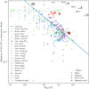 |
Fig. 4 |Pmin|–albedo relation. The legends are identical to those in Fig. 3. The transparent glass powder samples are shown as a range, with the grain size (D) at the ends indicated because the albedo for each sample was unavailable. For lunar observations, Pmin = Pr(α = 10.5°) is assumed (Shkuratov et al. 1992). For alumina samples, D/λ = 0.093 is enclosed in parentheses because their Pmin values are extrapolated values (GG90). |
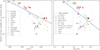 |
Fig. 5 Umov laws for mineral and silica mixture samples that use different albedo definitions. The square and diamond endmembers are from Spadaccia et al. (2022) and Sultana et al. (2023), respectively (see Sect. 2 for details). Silicate-carbon mixture samples and Ceres and Vesta are shown for comparison (see Fig. 3). The abbreviations are as follows: si: silica, mt: magnetite, spi: spinel, graph: graphite, fo: forsterite, fa: fayalite, ol: olivine, and FeS: iron sulfide. Binary and tertiary mixtures are indicated by connecting endmembers with a hyphen (“-”) in the legend. |
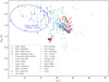 |
Fig. 6 Pmn-α0 parameter space plot for samples and lunar observations. The legends are the same as those in Fig. 4, and the typical location of rocky surfaces is indicated with a blue ellipse. Ceres and Vesta are shown for comparison (see Fig. 3; b = 0.30–0.45 µm). |
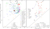 |
Fig. 7 Albedo-α0 relation. The legends on the left and right panels are identical to those in Figs. 3 and 5, respectively. The red letters on the right indicate the taxonomic types of asteroids of the letter, except “h” stands for the Ch-type (Belskaya et al. 2017). The “boundary” (Eq. (2)) is indicated by black dotted lines. Ceres and Vesta are shown for comparison (see Fig. 3). |
4.2 The D/λ upper bound for the WD trend
We showed the WD trend is observed across a broad spectrum of samples, not limited to alumina (Sect. 2.2; GG90). Now we review some additional publications that provide insights leading us toward a quantification of the upper boundary for the D/λ range within which the WD trend is observed.
A study by Muñoz et al. (2021) investigated the polarimetric properties of forsterite powders, encompassing a size range from 0.7 to ~100 µm, alongside 1600 µm pebbles. The emergence of the WD trend is observed as the particle size decreases, commencing at D/λ ~ 5–10.
Frattin et al. (2022) found that the NPB tends to become slightly stronger (the WD trend) for smaller particles in both olivine and spinel samples. The size frequency distribution of the samples (in their Fig. 2) indicates that their “small” sample corresponds to particles D ~ 2 µm (D/λ ~ 4), while their “medium” sample encompasses the “small” particles along with additional particles D ~ 25 µm. This mixture of particle sizes may contribute to the less distinct WD trend (i.e., small and medium samples both show similar NPB) in their study.
Figure 12 in Volten et al. (2001) presents an analysis of various aerosol samples, including red clay, quartz, Pinatubo ash, loess, and Lokon ash. The figure shows the WD trend for these samples as the wavelength increases from 0.4416 µm to 0.6328 µm. Notably, despite these samples having overall effective grain sizes of D ≲ 10µm, the strongest peaks in size-frequency distributions occur at D ~ 1–2 µm (as shown in their Fig. 1). This observation supported the existence of grains with values of D/λ that became conducive for the WD trend to occur.
Escobar-Cerezo et al. (2018) demonstrated that the NPB significantly diminishes when small (radius < 1 µm) particles are removed from lunar simulants. We estimated that the number of removed particles was 0.5 µm < D ≪ 10 µm from their size frequency distributions and microscopy images. Conversely, the addition of 1 < D/λ ≪ 20 particles induces a WD trend.
Combining all these results with those of the previous section, while also considering the properties of GG90 and context provided in our previous discussions, we propose that the WD trend is observed when D/λ ≲ 5–10. This trend can be a diagnostic indicator of the upper bound of the grain size on the scattering surface upon observing it with increasing λ. However, we acknowledge that this threshold value is rather uncertain and subjective. Further research can provide a clearer understanding of the exact dependencies in various scenarios. For example, the location where the ND trend starts to appear, the WD–ND transition point, is discussed in Sect. 6 after the other effects (especially that of albedo) are discussed.
5 Other effects on the negative branch (Pmin and α0)
Having explored the influence of D/λ on the NPB, we focus on other factors. Specifically, we discuss the effects of albedo, compression, and the refractive index.
5.1 Albedo
Figure 7 shows yet another parameter space, the albedo-α0 space, encompassing a diverse array of samples, including lunar observations (Shkuratov et al. 1992) and asteroid data (Belskaya et al. 2017). It is worth noting that while the specific numerical values may be arbitrary and the albedo definitions differ across studies, a discernible pattern emerges. We identify the following inequalities (the black dotted line in the figure):

for albedo A in natural units and α0 in degrees. Figure 4 in Shkuratov et al. (1992) also shows a similar “boundary” for water-color samples.
As already demonstrated in Fig. 1, α0 of alumina remains relatively constant with respect to albedo (for ≳ 20%) but changes only if D/ λ is varied. The same is true for transparent glass powder samples (albedo 40–60%). In the right panel of Fig. 7, it is shown that the mixture samples merely follow nearly vertical or L-shaped curves connecting their endmembers. The “Silicate+Carbon”, fo-graph and si-mt mixtures show nearly fixed α0 over a wide range of albedos. Moreover, the fo-spi and si-fo mixtures exhibited an α0 change, although the albedo was nearly fixed. All these findings emphasize that the albedo is not the only factor tuning α0. Neither is the albedo contrast (e.g., Sect. 4.6 of Spadaccia et al. 2022). From all the mixture samples, including those containing tertiary mixtures, we hypothesize that the minimum/maximum α0 is determined roughly by the endmember with the smallest/largest α0, except possibly for subi scale end-members (e.g., the ol-FeS samples and Shkuratov 1987). Further parameter spaces related to albedo and αmin are briefly discussed in Appendix A.
GG90 described the effect of decreasing albedo on deepening the NPB, citing Fig. 4 of Geake et al. (1984) that it is theoretically expected. Figures 8 and 9 are drawn specifically to emphasize the effect of albedo. From the figures, as well as Fig. 7, one finds the following general trends for albedo:
For lower albedo (≲2–10%), increasing albedo strengthens the NPB (WD-like).
For higher albedo (≳5–l0%), increasing albedo weakens the NPB (shallower Pmin), which is the classical expectation of the Umov law, while α0 does not change much.
We denote the first trend “WD-like” because we use the “WD trend” to indicate that D/λ is the primary cause of the observation. Therefore, the albedo trend for low-albedo objects can be combined with the WD trend, complicating the analyses (Sect. 5.2).
A qualitatively similar trend was reported in Fig. 22 of Shkuratov et al. (1994) for “metallic or semimetallic rough pulverized” samples and in Fig. 4 of Shkuratov et al. (1992) for mixtures of water color (λ = 0.65 µm). According to Shkuratov et al. (2002), the mixture of chalk and soot (D < 1 µm) at λ = 0.63 µm shows a deepening trend as adding soot decreases the albedo from 90% to 8%. This finding aligns with the albedo effect at higher albedos, as described above. The measured a range is limited in their work (up to 3.5°), so the width (α0) trend cannot be mentioned.
Among the two “Candle Soot”samples, the shallower NPB is described as “oosely piled”sample. The sample (MgO5 albedo 1.1%) lies between the two “Silicate+Carbon” mixtures of albedos 0.2 and 1.7%, which indicates that albedo is the primary parameter contributing to these effects. Another “Candle Soot” with the same albedo (deeper NPB) deviates from the trend of “Silicate+Carbon” because it is a pure deposit, that is, not prepared by “deliberately roughening”8 procedure.
The single “Rubber Soot” data have an H2 albedo of 2.6%. The sample is likely a pure deposit soot sample, which may explain why it is located near the pure deposit candle soot. The two “Soot[+MgO]” samples are prepared by shaking the test tubes rather than roughening the surface9. However, the two “Soot[+MgO]” samples still show a WD-like trend for increasing albedo, which is the trend for dark objects summarized above.
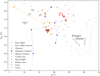 |
Fig. 8 Laboratory samples in Pmin−α0 (depth-width of NPB) space. Alumina samples are shown in Fig. 1. The numbers with units % are albedo values. “Silicate+Carbon” samples are connected by lines in the order of albedo. The arrows for “Pressed Albedo” indicate the increasing albedo for the pressed MgO and soot mixture sample given in the original publication. Ceres and Vesta are shown for comparison (see Fig. 3; b=0.30–0.45 µm). |
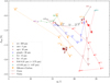 |
Fig. 9 Similar to Fig. 8 but different samples to emphasize the dependence of the NPB on albedo. Note that the axes ranges are slightly different. The endmembers are denoted by a filled square (Spadaccia et al. 2022) or filled diamond (Sultana et al. 2023). The dotted lines connect the mixtures in the order of albedo. The numbers indicate the reported “albedo” values. Ceres and Vesta are shown for comparison (see Fig. 3). |
5.2 Albedo vs. D/λ effects
As mentioned, the effects of albedo and D/λ may play roles simultaneously, and both contribute to widening and/or deepening, which complicates the analyses. We look into a few cases that highlight this complication.
Shkuratov et al. (2002) report interesting trends from two water colors and a Fe2O3 sample (all with D ~ 1 µm particles). As the wavelength increased from λ = 0.45 to 0.63 µm, the albedos and the NPB trends were reported as
Red water color: A = 7% and 68%, shallowing.
Blue water color: A = 43% and 24%, deepening.
Fe2O3 (reddish): A = 5% and 20%, no change.
The red water color follows the albedo trend of high-albedo objects. This is the opposite of the D/λ effect, which is expected to deepen. This might indicate that the albedo effect dominates the D/λ effect, as can be expected from its large change in albedo. Conversely, for the blue water color, deepening is anticipated from both the albedo and D/λ effects, thus posing no contradiction. In the case of the Fe2O3 sample, it is possible that the shallowing effect driven by albedo and the deepening effect due to D/λ counterbalance each other.
Among multiple samples, Volten et al. (2001) reported that feldspar grains exhibit no change in Pmin when λ = 0.4416 µm is changed to 0.6328 µm. Their sample had a D = 2 µm peak, which corresponds to D/λ = 4.5 and 3.3 for the two wavelengths. They described feldspar as having a “light pink” color, which coincides with the D = 2 µm feldspar sample albedos reported in Shkuratov et al. (2004): 67% and 88% in À = 0.45 and 0.63 µm, respectively. Thus, similar to the Fe2O3 sample discussed above, the albedo effect (shallowing) and the D/λ effect (deepening) may cancel each other out.
The fo-fa mixture in Fig. 9 exhibits a trend different from that of the general one, a strong widening pattern, contrary to the other typical behaviors observed in high-albedo objects. The microscopy images (Spadaccia et al. 2022) show that forsterite contains significantly finer structures down to the wavelength scale than does fayalite. This result indicates that the trend observed in the fo-fa mixture might be influenced by the grain size effect, wherein a reduction in D/λ toward forsterite contributes to widening, whereas the depth trend appears to be canceled out.
5.3 Compression
The compression process plays a dual role in influencing the behavior of the NPB, with its impact characterized by the simultaneous reduction in macroscopic roughness (if present) and a consequential decrease in interparticle distance, which reduces porosity. For example, when compressing “Soot+MgO”, we observe a WD-like trend (Fig. 8). A similar trend was observed 15 µm for the SiC powder (Fig. 13.14 of Hapke 2012). In both cases, the authors do not explicitly describe a roughening process, so compression affects porosity in this case.
The results presented in GG90 are based on alumina samples flattened by a spatula to control all the other parameters except D/λ (Sect. 2.2). The difference in the PPCs of different works using alumina samples (GG90, Poch et al. 2018, Shkuratov et al. 2002, Nelson et al. 2002, 2018, Ovcharenko et al. 2006) could also be due to the different processes of compression. The photomicrograph in Ovcharenko et al. (2006) hints that compression can indeed change the shapes of aggregates.
The effect of compression on the MgO coating is reported in Figs. 2 and 4 of Shkuratov et al. (2002). A sharp peak with αmin ≲ 1° is exhibited only for uncompressed samples. After mechanical compression, Pmin became shallower, and αmin and α0 increased (their Fig. 2). After drying-in-alcohol compression, Pmin remains the same, and αmin increases (likely α0, as shown in their Fig. 4, which seems to be identical to the sample shown in Fig. 2 in Shkuratov & Ovcharenko 2002). This difference may be related to the fine-scale structure that existed in the MgO coating (D ≪ 1 µm), which was responsible for the POE being removed after compression. We note that the availability of data points near the POE can distort the results. This shows the complication of NPB analyses for superfine particles unless we fully sample the PPC at small a. Figure 13 in Shkuratov et al. (2002) and Fig. 2 in Shkuratov & Ovcharenko (2002) also demonstrated that D = 0.01 µm silica shows a WD-like trend after compression, but one needs data at α < 1°, which is not available in most publications.
Inducing the WD-like trend is not the only possible effect of compression. For example, in the Appendix of Spadaccia et al. (2022), compression is shown to have the following additional effects:
Silica: WD-like.
Magnetite: Narrowing and shallowing.
Silica-magnetite 1:1 mixture: Width fixed and deepening.
Experiments with black plasticine sprinkled with dark glass powders showed a loss of NPB when the glass powders were carefully pressed into plasticine one by one (Fig. 13 in Geake et al. 1984). In this specific example, “compression” resulted in the elimination of multiple scattering by dark particles. Similarly, flattening the lunar fine (Apollo 10084-6) resulted in a weakening of its NPB (Fig. 10 in Geake et al. 1970). Moreover, in the study of terrestrial samples, Dollfus et al. (1971a) noted that “when the surface is flattened, the negative branch becomes less pronounced”10. Dollfus et al. (1969) described how compressing a limonite-goethite powder mixture (Mars simulant) resulted in shallower NPB, but there was no description about α0. All these findings are exactly the opposite of the WD-like behavior.
In the experiments involving lunar fine and terrestrial samples discussed here, compression involves not only a substantial decrease in porosity but also a notable reduction in surface roughness. This occurs because they compare “deliberately roughened” samples with corresponding pressed samples. Interestingly, Zellner et al. (1977a) reported that compaction did not “have any noticeable effects” on any of the meteoritic samples, except for the “highly translucent Norton County aubrite”.
5.4 Refractive index
Comparing Jovian satellites and lunar fines, GG90 suggested that increasing the real part of the refractive index (n) may result in a WD-like trend. (Earlier, Lyot 1929) described grain shape as likely to be a more important factor than the refractive index by comparing powdered calcite and precipitated chalk, crushed glass and spherical glass powders with sodium chloride. In Ishiguro et al. (2022), a deepening trend due to hydration was found, which may be related to the refractive index.
The distributions of alumina in Figs. 3 and 4 may bear some resemblance to the theoretical expectation for metals (high imaginary refractive index; Fig. 2 of Wolff 1980), and one may conclude that the imaginary part of the refractive index is the controlling parameter. However, alumina is a nonmetallic substance. Furthermore, multiple samples with D/λ = 0.093–75 were measured under the same filter (G), thus maintaining a constant refractive index yet still exhibiting deviations from the general trend. Thus, a change in the imaginary refractive index is unlikely to be the main cause of the difference between these samples and other samples.
Based on the findings of Masiero et al. (2009), Devogèle et al. (2018) argued that the change in n of spinel (1.81 and 1.78 at λ = 0.42 µm and 0.76 µm, respectively) may be affecting the narrowing trend of α0(λ) of the Barbarian asteroids. Can this be the cause of the WD and/or ND trend in Fig. 1?
Alumina is anticipated to show ∆n ≈ −0.02 (Sect. 2.3) from the B to I band (∆λ = 0.35 µm), while ∆α0 ≈ −5° in Fig. 1. Masiero et al. (2009) showed that, according to the theory of Muinonen et al. (2002a), the α0 value changes most significantly by n, but only a slight change is expected from the power-law particle size distribution. We first reproduced their results using the same formalism with a fixed power-law distribution with power −2.5, n = 1.77, and minimum and maximum sizes D ± 0.02 µm. We found that for D = 0.3 µm under the G filter, dα0/dn ≈ +1°/0.01. Thus, we expect ∆α0 = −2° under the given ∆λ. Second, if the case of spinel (Fig. 12 of Devogèle et al. 2018, which gives dα0/dn ~ +2°/0.01) is blindly applied, we expect ∆α0 ~ −4°. These two results appear to explain the observed ND trend to a certain degree. Moreover, in the case of spinel, ∆n ≲ −0.02 from the V- to J-/H-bands (Hosseini 2008; Devogèle et al. 2018), so it is expected that ∆α0 ≲ −4°. This interpretation coincides with the later observations of spinel-bearing asteroids in the J- and H-bands (Masiero et al. 2023).
However, we note that GG90 observed the WD trend only using the G filter, so ∆λ = 0 and An = 0 (Fig. 1). Moreover, the ND trend is also observed in the three G filter measurements. Therefore, both the WD and ND trends are observed without a change in n. As a result, we propose that the effect of D/λ is a simpler explanation. However, further experiments may be required to confirm these findings.
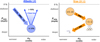 |
Fig. 10 Schematic diagram to visualize the trends in albedo and size (D/λ). The arrows for albedo (A; blue) and size (D/λ; orange) indicate the direction of increasing albedo and decreasing D/λ (increasing λ), respectively. |
6 Transition to the narrowing and deepening (ND) trend
We next consider the lower bound of D/λ at which the WD trend stops. We note that experiments involving D/λ ≲ 1 are relatively rare, and the particle size frequency distribution and microscopy images indicate challenges in achieving homogeneous grain sizes in this small regime. As a result, the ND trend itself is not as clear as the WD trend in the literature.
One of the earliest reports documenting the ND trend is shown in Fig. 5 of Dollfus et al. (1969; also Dollfus & Focas 1966). The mixture named “Adamcik A”, comprising a complex combination of fine-grained goethite, kaolin, hematite, and magnetite, showcases the ND trend when wavelengths increase from λ = 0.50 µm to 0.60 µm: (Pmin, α0) = (−0.75%, 24°) to (−0.9%, 20°). These two points lie closely on the ND trend of D = 0.3 µm alumina samples in Figs. 1 and 8. The authors, however, did not provide further details regarding this behavior due to the inability of the sample to replicate the Martian PPC.
The WD trend among transparent glass powders is shown from D/λ > 100 to D/λ ~ 1 (Fig. 6; Shkuratov et al. 1992). It is not definitively clear if D/λ = 1 represents the WD-ND transition point due to a lack of experiments involving smaller particles and because the transparency of the sample may make the physical processes different from those of regolith material. However, this finding does suggest the possibility that the transition may occur at a D/λ value less than 2.
Specifically, for alumina, Fig. 3 in Shkuratov & Ovcharenko (2002) reports the ND trend for alumina when comparing D = 1 µm and D = 0.1 µm samples under λ = 0.65 µm, as expected. Nelson et al. (2002, 2018) and Shkuratov et al. (2002) reported the deepening trend of the NPB as D/λ decreases. However, the PPC of the NPB in Nelson et al. (2018), spanning from D = 0.1–1.5 µm, does not show a clear trend in α0, as expected from the WD and ND trends. This difference may be related to other factors (such as the surface roughening process, grain shape, alignments, imperfect size segregation, and compression, as described in Sect. 5.3).
Therefore, the ND trend is not always clearly observed in the literature, as shown in Fig. 1. Combining the observations discussed thus far, we suggest that the WD trend stops (WD-ND transition) at D/λ ~ 1–2, although this requires further investigation.
7 A summary of grain size (d/λ) and albedo effects
Based on existing experimental findings in the academic literature, we examined the patterns within the Pmin−α0 space. The impacts of the two most important parameters, D/λ and albedo, are schematically depicted in Fig. 10.
Among these factors, we focus on the importance of the trend by D/λ because previous studies separately focused on analyzing the effects of D and λ. As λ increases, given that the albedo does not change significantly,
when the WD trend starts: D ≲ (5–10)λ,
when the WD trend slows down: D ~ (1–2)λ, and
when the ND trend appears: D < λ.
Based on the discussions and analyses presented throughout this study, it remains uncertain whether the D value derived from this logic corresponds to the most dominant grain size on the surfaces examined. For example, our investigation does not clearly tell whether a small amount of D = λ particles in the Daverage = 102 sample can induce clear WD and/or ND trends. To address this important question and gain a more comprehensive understanding of these dynamics, future experiments are necessary.
We also note that, the refractive index (and thus the albedo and reflectance) and interparticle distance in terms of wavelength units will change with λ. In extreme cases, such as those involving ice frost, objects with atmospheres, and near-Sun objects that may emit thermal emission at shorter wavelengths, our straightforward calculation may not be directly applicable. These complications deserve careful consideration and bespoke analyses to provide a more accurate interpretation of polarimetric observations in these contexts. Additionally, the distinction between “grain size” and “microscopic roughness” is not always sharply defined.
8 Application to celestial objects
Insights into how particle size influences the NPB, as detailed in the preceding sections, can be employed in reverse to estimate particle sizes (D) on airless bodies. We tested this phenomenon to validate the feasibility of this methodology. Possible applications for the Moon, Mercury and Mars are discussed. Finally, a brief discussion of a complementary approach involving thermal modeling is given. Extension to small bodies will be presented in our follow-up paper (Paper II).
8.1 Moon
8.1.1 Observations
Although some researchers have mentioned that there is no λ-dependence in the lunar NPB (e.g., Fig. 12 caption of Dollfus 1971), others have discussed this phenomenon. Among them, Gehrels et al. (1964) confirmed the Wd trend of the lunar NPB as λ increased from the U (0.36 µm) to the I (0.94 µm) band. Clarke (1965) reported the same WD trend from filter 94 (0.459 µm) to 89B (0.739 µm).
More recently, Shkuratov et al. (1992) clearly showed NPB changes over λ: The NPB is strengthened from blue (λ = 0.42 µm) to red (0.65 µm), as shown in Fig. 6. Figure 18 of Dollfus & Bowell (1971) shows that α0 changes significantly for the case of the Moon (α0 < 21° at λ = 0.327 µm to α0 ~ 26° at λ = 1.05 µm, and a marginal hint that it remains constant for λ ≳ 1 µm). Although they reported that “neither Pmin nor αmin change significantly with wavelength", the change in α0 is qualitatively similar to the change in the lunar regions shown in Fig. 6.
8.1.2 Interpretations
Because the change in albedo with wavelength is significant for all four types of lunar surfaces, the effect of albedo should be considered. For maria (albedo ≲10%), a WD-like trend is observed when as λ increases, aligning with both the albedo trend of darker objects and the effect of decreased D/λ. For the higher albedo (> 10%) regions, however, Pmin does not change much, while a0 clearly increases. The albedo effect expects shallowing of the NPB; thus, as for the case of Fe2O3 (Sect. 5.2), we can infer that both the albedo and D/λ effects simultaneously and effectively cancel each other except for the increase α0.
If the D/λ effect genuinely impacts the NPB, we can estimate the grain size based on these observations. A WD trend of D/λ starting from the U-band to the B-band indicates grains of D ≲ (5–10)λ ≈ 2–4 µm. Moreover, α0 starts to become constant for λ > 1 µm (Dollfus & Bowell 1971; Sect. 8.1.1), that is, the WD-ND transition. From this, we propose that D ~ (1–2)λ ≈ 1–2 µm affects the NPB, which is consistent with the conclusion drawn from the WD trend.
The grain sizes estimated by the two methods agree well with the size-frequency distribution analyses of lunar fine samples (Park et al. 2008). This alignment emphasizes that estimating grain size using the initiation of the WD trend is a reliable approach. This further indicates that employing multiwavelength observations of NPB to estimate grain size is a useful approach.
8.2 Mercury
Although Mercury was observed at multiple wavelengths (Dollfus 1961; Dollfus & Auriere 1974), the NPB was well covered at only one wavelength, and the PPC near the inversion was available only between 0.520 and 0.630 µm at one location. Given the scatter of the data, we cannot find a hint of a change in α0 (change < 1–2°). Dollfus & Auriere (1974) concluded that Mercury has a PPC similar to that of the lightest lunar mare fine, that is, ∆α0 ≲ 1° given the wavelength range, according to Dollfus & Bowell (1971). Thus, more precise multiwavelength polarimetry in the NPB can shed light on the grain properties of Mercury.
8.3 Mars
With its thin atmosphere, Mars technically falls outside the scope of our current work. Even so, it is intriguing that multiwavelength polarimetry was conducted on clear and pure surface regions on Mars11 reveals a definitive change in the NPB (Dollfus & Focas 1969, 1966; Dollfus et al. 1969). After digitizing their data, we added a data point (α, Pr) = (0°, 0%). Because of the lack of data near a0 for certain wavelengths, we calculated the polarimetric parameters by two fitting methods: a linear-exponential function and a spline fit. The average of these values was taken, and half of the differences between these two values were regarded as the initial error bars. From visual inspection to the PPCs, ∆Pmin ~ 0.1 %p and ∆α0 ~ 1° are expected (e.g., data points with Pr< Pmin − 0.2 %p). We calculated the final error bar by propagating these values as an additional random error. Moreover, from the reflectance spectra (McCord et al. 1982; Mustard & Bell 1994; Erard & Calvin 1997; Bell & Ansty 2007), we obtained representative (mean) reflectance values, r(λ). The possible ranges (bright and dark regions) at each wavelength are extracted by visual inspection and regarded as error bars. The derived parameters are plotted in four parameter spaces in Fig. 11.
The trajectory of Mars in the Pmin−α0 space displays a typical albedo trend from albedo < 5% to ~30% (Fig. 10; Sect. 5.1). For longer wavelengths, the albedo remains nearly constant. Thus, if the D/λ effect is effective, the NPB must change at the longest wavelengths. Considering that a0 remains unchanged while λ is changed by a factor of ~2, it is likely that D/λ ≫ 10 is maintained up to λ = 1.05 µm, that is, D ≫ 10 µm. Another possible explanation could be the WD-ND transition at λ = 0.6–1.05 µm, which translates to D ~ 0.6–1.2 µm or 1.05–2.1 µm.
Notably, D > 10 µm was obtained based on the Pmax-albedo relationship and thermal modeling for a few selected regions on Mars (Dollfus et al. 1993). Thus, we prefer the first interpretation that the trace of Mars in the parameter space is driven by the albedo effect, not by the D/λ effect, because the grain sizes are too large.
Due to the atmospheric disturbances on Mars, the PPC may not represent the bare surface, even though measurements were deliberately selected based on monitoring the clearest regions. Thus, we refrain from providing further quantitative estimations related to Mars in this context. Instead, we propose that a future near-infrared polarimetry investigation considering regional variation could provide a conclusive perspective on this topic.
8.4 Thermal modeling: A complementary approach
As discussed in Sect. 1, thermal modeling is also used for indirect measurements of particle sizes. The temperature distribution on an asteroid can be calculated using thermophysical models (TPMs), such as those developed by Dickel (1979) and Spencer et al. (1989). This temperature distribution, and the corresponding thermal flux, is closely related to the thermal inertia  , thermal conductivity k, mass density ρ, and specific heat capacity cs.
In the simplest case, a lower Γ value indicates less efficient thermal conduction, which can be interpreted as smaller grain sizes in the regolith (Mellon et al. 2000). The Hayabusa2 mission, which included the MASCOT lander (Tsuda et al. 2013; Watanabe et al. 2017), landed on the asteroid (162173) Ryugu. The surface temperature profile from MASCOT’s observations revealed that fine grains should not cover surfaces thicker than 50 µm (Grott et al. 2019). An identical < 50 µm thickness requirement was found for (101955) Bennu from OSIRIS-REx observations (Rozitis et al. 2020), and it was concluded that its surface is mostly covered with meter-scale boulders (Dellagiustina et al. 2019).
A more realistic model developed by Gundlach & Blum (2013) provides a methodology for calculating thermal conductivity by considering the solid spherical particle contact theory and the radiative conduction of opaque particles. This calculation requires assumptions about the properties of the grain, such as Young’s modulus, Poisson’s ratio, mass density, specific heat capacity, and hemispherical infrared emissivity. These values are assumed and fixed based on the spectral type information of the asteroid. By treating the porosity and grain size as free parameters, the thermal flux of the asteroid can be calculated. Various studies have applied this approach (Davidsson et al. 2015; Hanuš et al. 2018; Delbo et al. 2015 and references therein). Recently, MacLennan & Emery (2022b,a) successfully utilized this method to analyze a wide range of asteroids and retrieve information about grain sizes.
This forward modeling approach faces challenges in accurately representing complex reality. One example is the calibration of correction factors, such as the “χ factor” in Gundlach & Blum (2013), which is a multiplication factor to match theory to experiment, based solely on lunar fines data from Apollo 11’s 10084-68 (Cremers et al. 1970) and Apollo 12's 12001,19 (Cremers & Birkebak 1971). Another challenge arises from the temperature dependence of properties such as cs and k (MacLennan & Emery 2022b). Furthermore, the exact determination of thermal inertia through forward modeling relies on data fitting, which is sensitive to observations (bandpass filters, sampling density, etc.) and specific model settings, such as roughness (Davidsson & Rickman 2014) and shape models (Hanuš et al. 2015), which in turn affect particle size determination.
Consequently, while forward modeling offers valuable insights into the underlying physics of observations, it has its own limitations. Thus, alternative independent and empirical approaches such as the polarimetric studies presented in this work hold great value in complementing our understanding. As we have shown, our methodology is sensitive only to particles D ≲ 10λ, which is a limitation compared to the thermal modeling approach. In Paper II, we will discuss our polarimetric observations and analyses, highlighting their strong alignment with grain size estimations derived from an independent methodology by thermal modeling, showcasing the validity of the two approaches. These complementary analyses offer valuable insights, enhancing our understanding of the studied phenomena.
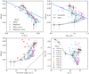 |
Fig. 11 Polarimetric parameters of Mars compared to those of the Moon and asteroids. The Mars data are connected in the order of wavelength. The dotted line in the albedo–α0 space is the same as Fig. 7 (Eq. (2)). |
9 Conclusions and future work
In this study, we summarized the effect of physical parameters on the shape of the NPB based on previous experimental and observational studies. The NPB trends are summarized below (also see Fig. 10):
With increasing albedo A, the NPB exhibited a WD trend until A ~ 2–10%. The NBP becomes shallower for A ≳ 5–10%, which is the expectation of the classical Umov law.
With decreasing D/λ: The NPB stays fixed for D/λ ≫ 10. The WD trend starts at D/λ ~ 5–10. This trend slows down at D/λ ~ 1–2, and the ND trend may be observed at D/λ ≲ λ.
The effect of compression (roughness, multiple scattering, and porosity) is case dependent and requires further study.
The effect of the real part of the refractive index (n) can explain the ND trend, but the D/λ effect is a simpler explanation.
In particular, we leveraged the D/λ effect to estimate the grain size of selected celestial objects, and the method yielded highly satisfactory results, particularly for the case of the Moon (and Mars). Additionally, we emphasize D/λ and that albedo effects can complicate the interpretation of the observed WD trend.
Future laboratory experiments can shed light on the study of regolith on airless bodies. This can include investigating (i) separating the D/λ and albedo trends (e.g., using flat reflectance materials), (ii) examining how mixing identical ingredients with different particle sizes influences polarization, (iii) disentangling the contributions of porosity and roughness to the observed polarization, and (iv) designing experiments specifically to quantify the albedo and D/λ trends suggested here.
While doing so, maintaining narrow size frequency distributions for each sample can be important, though practically challenging. All other investigations into any parameter space merit science. To ensure the comparability of results across studies, the adoption of a unified protocol for specifying wavelengths and measuring key polarization parameters, such as Pmin, αmin, α0, h, and albedo, is paramount (e.g., different definitions of h and albedo complicate direct comparisons). The introduction of set of widely acceptable parameters related to the skewness of the NPB may shed light on POE. Standardization can enable researchers to draw more robust conclusions and advance our understanding of polarization phenomena.
In the domain of observational science, the study of near-infrared polarimetry methods for asteroids is still in its infancy, with recent studies marking the initial steps in this field (Masiero et al. 2022, 2023; Paper II). As noted above, it is crucial to delineate the distinct influences of albedo and D/λ effects. To enhance our understanding, we propose a focus on objects where the albedo effect could be separated. We initiated preliminary observations of specific large airless bodies from 2019 to 2021, unaware of the concurrent investigations. In the forthcoming paper of this series (Paper II), we aim to employ the methodologies established in this work to explore airless objects from an observational viewpoint. This approach will advance our understanding of these cosmic bodies.
Acknowledgements
This work was supported by a National Research Foundation of Korea (NRF) grant funded by the Korean government (MEST) (No. 2023R1A2C1006180). Y.P.B. would like to thank Angélique Pathammavong for a valuable contribution in creating the summary figure. The authors want to thank Joseph Masiero for providing constructive comments as a referee.
Appendix A Parameter Space Related to αmin
Figa. A.1, A.2, and A.3 are similar to Fig. 7 but with αmin and α0 − αmin, and the skewness S : = 1 − αmin/α0 (larger S value may indicate a strong POE) on the abscissa. Interestingly, the mixture samples show a tighter relationship in the latter two parameter spaces. Additionally, asteroids (Belskaya et al. 2017) and Mars (Sect. 8.3) are located in very similar locations. Even the L-type that shows a distinctive location in the albedo-α0 space is now located in the general trend for the latter two diagrams. The asteroids and Mars generally had less skewed NPB than did the laboratory samples (especially 0.5 ≲ S ≲ 0.6 for albedo ≲ 30% objects).
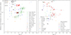 |
Fig. A.1 Same as Fig. 7 but with α0 − αmin. The αmin values are from Belskaya et al. (2017), while that of Q-type is adopted for (214869) 2007 VA8 (Gil-Hutton 2017; http://gcpsj.sdf-eu.org/catalogo.html). Ceres and Vesta are shown for comparison (see Fig. 3). Data points for Mars are connected in the order of increasing wavelength. |
References
- Bach, Y. P., Ishiguro, M., Jin, S., et al. 2019, J. Kor. Astron. Soc., 52, 71 [NASA ADS] [Google Scholar]
- Bach, Y. P., Ishiguro, M., Takahashi, J., et al. 2024, A&A, 684, A81, (Paper II) [NASA ADS] [CrossRef] [EDP Sciences] [Google Scholar]
- Beck, P., Schmitt, B., Potin, S., Pommerol, A., & Brissaud, O. 2021, Icarus, 354, 114066 [NASA ADS] [CrossRef] [Google Scholar]
- Bell, J. F., & Ansty, T. M. 2007, Icarus, 191, 581 [NASA ADS] [CrossRef] [Google Scholar]
- Belskaya, I. N., Shkuratov, Y. G., Efimov, Y. S., et al. 2005, Icarus, 178, 213 [NASA ADS] [CrossRef] [Google Scholar]
- Belskaya, I., Cellino, A., Gil-Hutton, R., Muinonen, K., & Shkuratov, Y. 2015, in Asteroids IV, eds. P. Michel, F. E. DeMeo, & W. F. Bottke, 151 [Google Scholar]
- Belskaya, I. N., Fornasier, S., Tozzi, G. P., et al. 2017, Icarus, 284, 30 [Google Scholar]
- Bohren, C. F., & Huffman, D. R. 1983, Absorption and Scattering of Light by Small Particles, (New York, Wiley-Interscience) [Google Scholar]
- Bowell, E., Dollfus, A., Zellner, B., & Geake, J. E. 1973, Lunar Planet. Sci. Conf. Proc., 4, 3167 [Google Scholar]
- Brewster, D. 1863, Trans. Roy. Soc. Edinb., 23, 205 [CrossRef] [Google Scholar]
- Cellino, A., Bagnulo, S., Gil-Hutton, R., et al. 2015, MNRAS, 451, 3473 [NASA ADS] [CrossRef] [Google Scholar]
- Clarke, D. 1965, MNRAS, 130, 83 [NASA ADS] [CrossRef] [Google Scholar]
- Cremers, C. J., & Birkebak, R. C. 1971, Lunar Planet. Sci. Conf. Proc., 2, 2311 [NASA ADS] [Google Scholar]
- Cremers, C. J., Birkebak, R. C., & Dawson, J. P. 1970, Geochim. Cosmochim. Acta Suppl., 1, 2045 [Google Scholar]
- Dabrowska, D. D., Muñoz, O., Moreno, F., et al. 2015, Icarus, 250, 83 [NASA ADS] [CrossRef] [Google Scholar]
- Daly, R. T., Ernst, C. M., Barnouin, O. S., et al. 2023, Nature, 616, 443 [CrossRef] [Google Scholar]
- Davidsson, B. J. R., & Rickman, H. 2014, Icarus, 243, 58 [NASA ADS] [CrossRef] [Google Scholar]
- Davidsson, B. J. R., Rickman, H., Bandfield, J. L., et al. 2015, Icarus, 252, 1 [Google Scholar]
- Delbo, M., Mueller, M., Emery, J. P., Rozitis, B., & Capria, M. T. 2015, in Asteroids IV, eds. P. Michel, F. E. DeMeo, & W. F. Bottke, 107 [Google Scholar]
- Dellagiustina, D. N., Emery, J. P., Golish, D. R., et al. 2019, Nat. Astron., 3, 341 [CrossRef] [Google Scholar]
- Devogèle, M., Cellino, A., Borisov, G., et al. 2018, MNRAS, 479, 3498 [Google Scholar]
- Dickel, J. R. 1979, in Asteroids, eds. T. Gehrels, & M. S. Matthews, 212 [Google Scholar]
- Dodge, M. J. 1986, in CRC Handbook of Laser Science and Technology, 4. Optical materials, Part 2 - Properties, ed. M. J. Weber (CRC Press), 21 [Google Scholar]
- Dollfus, A. C. 1955, PhD thesis, Université Pierre et Marie Curie (Paris VI), France [Google Scholar]
- Dollfus, A. 1956, Annales d’Astrophysique, 19, 83 [Google Scholar]
- Dollfus, A. 1961, in Planets and Satellites, eds. G. P. Kuiper, & B. M. Middlehurst, 343 [Google Scholar]
- Dollfus, A. 1971, in Physical Studies of Minor Planets, ed. T. Gehrels, (Washington, D.C.: National Aeronautics and Space Administration), 95 [Google Scholar]
- Dollfus, A., & Auriere, M. 1974, Icarus, 23, 465 [NASA ADS] [CrossRef] [Google Scholar]
- Dollfus, A., & Bowell, E. 1971, A&A, 10, 29 [NASA ADS] [Google Scholar]
- Dollfus, A., & Deschamps, M. 1986, Icarus, 67, 37 [NASA ADS] [CrossRef] [Google Scholar]
- Dollfus, A., & Focas, J. H. 1966, Polarimetric Study of the Planet Mars (US Air Force Cambridge Research Laboratories) [Google Scholar]
- Dollfus, A., & Focas, J. 1969, A&A, 2, 63 [NASA ADS] [Google Scholar]
- Dollfus, A., & Geake, J. E. 1975, Lunar Planet. Sci. Conf. Proc., 3, 2749 [Google Scholar]
- Dollfus, A., & Geake, J. E. 1977, Philos. Trans. Roy. Soc. Lond. Ser. A, 285, 397 [NASA ADS] [CrossRef] [Google Scholar]
- Dollfus, A., & Zellner, B. 1979, in Asteroids, (Tucson: University of Arizona Press), 170 [Google Scholar]
- Dollfus, A., Focas, J., & Bowell, E. 1969, A&A, 2, 105 [NASA ADS] [Google Scholar]
- Dollfus, A., Bowell, E., & Titulaer, C. 1971a, Astron. Astrophys., 10, 450 [NASA ADS] [Google Scholar]
- Dollfus, A., Geake, J. E., & Titulaer, C. 1971b, Lunar Planet. Sci. Conf. Proc., 2, 2285 [Google Scholar]
- Dollfus, A., Wolff, M., Geake, J. E., Lupishko, D. F., & Dougherty, L. M. 1989, in Asteroids II, eds. R. P. Binzel, T. Gehrels, & M. S. Matthews, 594 [Google Scholar]
- Dollfus, A., Deschamps, M., & Zimbelman, J. R. 1993, J. Geophys. Res., 98, 3413 [NASA ADS] [CrossRef] [Google Scholar]
- Dougherty, L. M., & Geake, J. E. 1994, MNRAS, 271, 343 [NASA ADS] [CrossRef] [Google Scholar]
- Erard, S., & Calvin, W. 1997, Icarus, 130, 449 [NASA ADS] [CrossRef] [Google Scholar]
- Escobar-Cerezo, J., Muñoz, O., Moreno, F., et al. 2018, ApJ, 235, 19 [NASA ADS] [Google Scholar]
- Frattin, E., Martikainen, J., Muñoz, O., et al. 2022, MNRAS, 517, 5463 [NASA ADS] [CrossRef] [Google Scholar]
- Geake, J. E., & Dollfus, A. 1986, MNRAS, 218, 75 [NASA ADS] [Google Scholar]
- Geake, J. E., & Geake, M. 1990, MNRAS, 245, 46 [NASA ADS] [Google Scholar]
- Geake, J. E., Dollfus, A., Garlick, G. F. J., et al. 1970, Geochim. Cosmoch. Acta Suppl., 1, 2127 [NASA ADS] [Google Scholar]
- Geake, J. E., Geake, M., & Zellner, B. H. 1984, MNRAS, 210, 89 [NASA ADS] [CrossRef] [Google Scholar]
- Geem, J., Ishiguro, M., Takahashi, J., et al. 2022, MNRAS, 516, L53 [NASA ADS] [CrossRef] [Google Scholar]
- Geem, J., Ishiguro, M., Granvik, M., et al. 2023, MNRAS, 525, L17 [NASA ADS] [CrossRef] [Google Scholar]
- Gehrels, T., Coffeen, T., & Owings, D. 1964, AJ, 69, 826 [NASA ADS] [CrossRef] [Google Scholar]
- Gil-Hutton, R. 2017, in ACM (Asteroid, Comets, Meteors) 2017, Montevideo, Poster1.d.17 [Google Scholar]
- Grott, M., Knollenberg, J., Hamm, M., et al. 2019, Nat. Astron., 3, 971 [Google Scholar]
- Gundlach, B., & Blum, J. 2013, Icarus, 223, 479 [Google Scholar]
- Hadamcik, E., Renard, J. B., Levasseur-Regourd, A. C., et al. 2009, J. Quant. Spectrosc. Radiat. Transfer, 110, 1755 [NASA ADS] [CrossRef] [Google Scholar]
- Hadamcik, E., Renard, J. B., Lasue, J., Levasseur-Regourd, A. C., & Ishiguro, M. 2023, MNRAS, 520, 1963 [NASA ADS] [CrossRef] [Google Scholar]
- Hanuš, J., Delbo', M., Durech, J., & Alí-Lagoa, V. 2015, Icarus, 256, 101 [CrossRef] [Google Scholar]
- Hanuš, J., Delbo', M., Durech, J., & Alí-Lagoa, V. 2018, Icarus, 309, 297 [CrossRef] [Google Scholar]
- Hapke, B. 2012, Theory of Reflectance and Emittance Spectroscopy (Cambridge University Press) [Google Scholar]
- Hosseini, S. M. 2008, Physica Status Solidi B Basic Res., 245, 2800 [NASA ADS] [CrossRef] [Google Scholar]
- Ishiguro, M., Kuroda, D., Watanabe, M., et al. 2017, AJ, 154, 180 [Google Scholar]
- Ishiguro, M., Bach, Y. P., Geem, J., et al. 2022, MNRAS, 509, 4128 [Google Scholar]
- Ito, T., Ishiguro, M., Arai, T., et al. 2018, Nat. Commun., 9, 2486 [Google Scholar]
- Kenknight, C. E., Rosenberg, D. L., & Wehner, G. K. 1967, J. Geophys. Res., 72, 3105 [NASA ADS] [CrossRef] [Google Scholar]
- Le Bertre, T., & Zellner, B. 1980, Icarus, 43, 172 [NASA ADS] [CrossRef] [Google Scholar]
- Levasseur-Regourd, A.-C., Renard, J.-B., Shkuratov, Y., & Hadamcik, E. 2015, in Polarimetry of Stars and Planetary Systems (Cambridge University Press), 35 [Google Scholar]
- Lupishko, D. F. 2018, Solar Syst. Res., 52, 98 [NASA ADS] [CrossRef] [Google Scholar]
- Lupishko, D. F., & Belskaya, I. N. 1989, Icarus, 78, 395 [NASA ADS] [CrossRef] [Google Scholar]
- Lyot, B. 1929, PhD thesis, Université Pierre et Marie Curie (Paris VI), France [Google Scholar]
- MacLennan, E. M., & Emery, J. P. 2022a, Planet. Sci. J., 3, 263 [NASA ADS] [CrossRef] [Google Scholar]
- MacLennan, E. M., & Emery, J. P. 2022b, Planet. Sci. J., 3, 47 [NASA ADS] [CrossRef] [Google Scholar]
- Malitson, I. H. 1962, J. Opt.l Soc. Am., 52, 1377 [NASA ADS] [CrossRef] [Google Scholar]
- Malitson, I. H., & Dodge, M. J. 1972, J. Opt. Soc. Am., 62, 1405 [Google Scholar]
- Masiero, J., Hartzell, C., & Scheeres, D. J. 2009, AJ, 138, 1557 [NASA ADS] [CrossRef] [Google Scholar]
- Masiero, J. R., Tinyanont, S., & Millar-Blanchaer, M. A. 2022, Planet. Sci. J., 3, 90 [NASA ADS] [CrossRef] [Google Scholar]
- Masiero, J. R., Devogèle, M., Macias, I., Castaneda Jaimes, J., & Cellino, A. 2023, Planet. Sci. J., 4, 93 [NASA ADS] [CrossRef] [Google Scholar]
- McCord, T. B., Clark, R. N., & Singer, R. B. 1982, J. Geophys. Res., 87, 3021 [NASA ADS] [CrossRef] [Google Scholar]
- Mellon, M. T., Jakosky, B. M., Kieffer, H. H., & Christensen, P. R. 2000, Icarus, 148, 437 [NASA ADS] [CrossRef] [Google Scholar]
- Muñoz, O., Frattin, E., Jardiel, T., et al. 2021, ApJS, 256, 17 [CrossRef] [Google Scholar]
- Muinonen, K. O. 1990, PhD thesis, University of Helsinki, Finland [Google Scholar]
- Muinonen, K., Piironen, J., Shkuratov, Y. G., Ovcharenko, A., & Clark, B. E. 2002, in Asteroids III, eds. W. F. Bottke Jr., A. Cellino, P. Paolicchi, & R. P. Binzel, 123 [CrossRef] [Google Scholar]
- Muinonen, K., Videen, G., Zubko, E., & Shkuratov, Y. 2002a, Numerical Techniques for Backscattering by Random Media, eds. G. Videen, & M. Kocifaj (Dordrecht: Springer Netherlands), 261 [Google Scholar]
- Muinonen, K., Videen, G., Zubko, E., & Shkuratov, Y. 2002b, in Optics of Cosmic Dust, eds. G. Videen. & M. Kocifaj, 261 [CrossRef] [Google Scholar]
- Mustard, J. F., & Bell, J. F. 1994, Geophys. Res. Lett., 21, 353 [NASA ADS] [CrossRef] [Google Scholar]
- Nelson, R. M., Smythe, W. D., Hapke, B. W., & Hale, A. S. 2002, Planet. Sci. J., 50, 849 [NASA ADS] [Google Scholar]
- Nelson, R. M., Boryta, M. D., Hapke, B. W., et al. 2018, Icarus, 302, 483 [NASA ADS] [CrossRef] [Google Scholar]
- Ovcharenko, A. A., Bondarenko, S. Y., Zubko, E. S., et al. 2006, JQSRT, 101, 394 [NASA ADS] [CrossRef] [Google Scholar]
- Park, J., Liu, Y., Kihm, K. D., & Taylor, L. A. 2008, J. Aerospace Eng., 21, 266 [CrossRef] [Google Scholar]
- Poch, O., Cerubini, R., Pommerol, A., Jost, B., & Thomas, N. 2018, J. Geophys. Res. Planets, 123, 2564 [NASA ADS] [CrossRef] [Google Scholar]
- Querry, M. R. 1985, Optical constants, Contractor Report, Sep. 1982-May 1984, Missouri Univ., Kansas City [Google Scholar]
- Rozitis, B., Ryan, A. J., Emery, J. P., et al. 2020, Sci. Adv., 6, eabc3699 [NASA ADS] [CrossRef] [Google Scholar]
- Shkuratov, Y. G. 1987, Sov. Astron. Lett., 13, 182 [Google Scholar]
- Shkuratov, Y. G. 1989, Solar Syst. Res., 23, 111 [NASA ADS] [Google Scholar]
- Shkuratov, Y. G., & Ovcharenko, A. V. 2002, Experimental Modeling of Opposition Effect and Negative Polarization of Regolith-Like Surfaces, eds. G. Videen, & M. Kocifaj (Dordrecht: Springer Netherlands), 225 [Google Scholar]
- Shkuratov, Y. G., Akimov, L. A., & Tishkovets, V. P. 1984, Sov. Astron. Lett., 10, 331 [Google Scholar]
- Shkuratov, I. G., Opanasenko, N. V., & Kreslavskii, M. A. 1992, Icarus, 95, 283 [NASA ADS] [CrossRef] [Google Scholar]
- Shkuratov, Y. G., Muinonen, K., Bowell, E., et al. 1994, Earth Moon and Planets, 65, 201 [NASA ADS] [CrossRef] [Google Scholar]
- Shkuratov, Y., Ovcharenko, A., Zubko, E., et al. 2002, Icarus, 159, 396 [CrossRef] [Google Scholar]
- Shkuratov, Y., Ovcharenko, A., Zubko, E., et al. 2004, JQSRT, 88, 267 [NASA ADS] [CrossRef] [Google Scholar]
- Shkuratov, Y., Bondarenko, S., Ovcharenko, A., et al. 2006, JQSRT, 100, 340 [NASA ADS] [CrossRef] [Google Scholar]
- Shkuratov, Y., Bondarenko, S., Kaydash, V., et al. 2007, JQSRT, 106, 487 [NASA ADS] [CrossRef] [Google Scholar]
- Spadaccia, S., Patty, C. H. L., Capelo, H. L., Thomas, N., & Pommerol, A. 2022, A&A, 665, A49 [NASA ADS] [CrossRef] [EDP Sciences] [Google Scholar]
- Spadaccia, S., Patty, C. H. L., Thomas, N., & Pommerol, A. 2023, Icarus, 396, 115503 [NASA ADS] [CrossRef] [Google Scholar]
- Spencer, J. R., Lebofsky, L. A., & Sykes, M. V. 1989, Icarus, 78, 337 [Google Scholar]
- Sultana, R., Poch, O., Beck, P., et al. 2023, Icarus, 395, 115492 [NASA ADS] [CrossRef] [Google Scholar]
- Tapping, J., & Reilly, M. L. 1986, J. Opt. Soc. Am. A, 3, 610 [NASA ADS] [CrossRef] [Google Scholar]
- Tropf, W. J., & Thomas, M. E. 1997, in Handbook of Optical Constants of Solids, III, ed. E. D. Palik (Burlington: Academic Press), 653 [CrossRef] [Google Scholar]
- Tsuda, Y., Yoshikawa, M., Abe, M., Minamino, H., & Nakazawa, S. 2013, Acta Astronautica, 91, 356 [CrossRef] [Google Scholar]
- Umow, v. N. 1905, Physikalische Zeitschrift, 6, 674 [Google Scholar]
- Vedam, K., Kirk, J. L., & Achar, B. N. N. 1975, J. Solid State Chem. France, 12, 213 [CrossRef] [Google Scholar]
- Veverka, J., & Noland, M. 1973, Icarus, 19, 230 [NASA ADS] [CrossRef] [Google Scholar]
- Volten, H., Muñoz, O., Rol, E., et al. 2001, J. Geophys. Res., 106, 17375 [NASA ADS] [CrossRef] [Google Scholar]
- Watanabe, S.-i., Tsuda, Y., Yoshikawa, M., et al. 2017, Space Sci. Rev., 208, 3 [Google Scholar]
- Weber, M. J. 2002, Handbook of Optical Materials (CRC Press) [CrossRef] [Google Scholar]
- Widorn, T. 1967, Annalen der Universitaets-Sternwarte Wien, Dritter Folge, 27, 109 [NASA ADS] [Google Scholar]
- Wolff, M. 1975, Appl. Opt., 14, 1395 [NASA ADS] [CrossRef] [Google Scholar]
- Wolff, M. 1980, Icarus, 44, 780 [NASA ADS] [CrossRef] [Google Scholar]
- Wolff, M. 1981, Appl. Opt., 20, 2493 [CrossRef] [Google Scholar]
- Worms, J. C., Renard, J. B., Hadamcik, E., Brun-Huret, N., & Levasseur-Regourd, A. C. 2000, Planet. Space Sci., 48, 493 [NASA ADS] [CrossRef] [Google Scholar]
- Zellner, B., Leake, M., Lebertre, T., Duseaux, M., & Dollfus, A. 1977a, Lunar Planet. Sci. Conf. Proc., 1, 1091 [Google Scholar]
- Zellner, B., Lebertre, T., & Day, K. 1977b, Lunar Planet. Sci. Conf. Proc., 1, 1111 [Google Scholar]
Spadaccia (2023; priv. comm.), https://zenodo.org/record/7550710
Poch (2023, priv. comm.), https://zenodo.org/record/7649167, and Beck (2023, priv. comm.).
58% albedo, Pmin = −0.6%, αmin = 3°, α0 = 10°, and Pmax = 21.7% were obtained from Yonne, France. Geake & Dollfus (1986) report slightly different values, so we adopt these original values based on the PPC.
MgO, 100% albedo, Pmin = −1.1%, αmin = 0.7°, α0 = 23°, Pmax = 8.2% (Lyot 1929). Although not plotted, the 0–10–1 slope h ~ 0.05%/°from Fig. 2 of Shkuratov et al. (2002).
Geake et al. (1970), above Fig. 9.
The “Rubber Soot” and “Soot[+MgO]” samples have H2 albedos of 2.6%, 3.6% and 4.3% (5wt% MgO). From the photometric phase curve of soot in Fig. 20 of Shkuratov et al. (2002), (albedo at a = 5°)/(albedo at a = 2°) ~ 0.91, if the halon has a flat intensity phase curve from a = 2–5°. Applying this approach to all three samples, the MgO5-equivalent albedos are 2.4%, 3.3%, and 3.9%, respectively.
All Tables
All Figures
|
Fig. 1 Laboratory samples in Pmin-α0 (depth-width of NPB) space. The numbers to the right of the alumina indicate D/λ and the filter, while the blue numbers to the left (with unit %) are the albedo values. D/λ = 0.093 data points are enclosed in parentheses because their Pmin values are extrapolated values. The WD and ND trends, with increasing λ (or decrease D/λ), are schematically indicated. |
| In the text | |
|
Fig. 2 Refractive indices of alumina (Al2O3) from various sources (see text for details). Available measurements closest to the central wavelengths of the filter (B, G, R, and I used in GG90) are indicated with markers. |
| In the text | |
|
Fig. 3 Slope (h)-albedo relation. See Sect. 2 and Table 1 for the details of the laboratory data and their original sources. The numbers next to the alumina samples are the D/λ values. The telescopic lunar observation data from Shkuratov et al. (1992) are shown for blue (0.42 µm) and red (0.65 µm) wavelengths using cyan and magenta colors, respectively, and the same regions are connected by a thin line. The lunar albedo is defined at α = 3.1°, so it should be smaller than the geometric albedo. The blue solid line is the regression line for asteroids (Lupishko 2018). The Ceres and Vesta results are shown as red and dark red, respectively, and are connected in the order of increasing wavelength: υ = 0.45–0.60 µm, r = 0.60–0.75 µm, i = 0.75−1.0 µm, J-, H-, and K-bands (Paper II). |
| In the text | |
|
Fig. 4 |Pmin|–albedo relation. The legends are identical to those in Fig. 3. The transparent glass powder samples are shown as a range, with the grain size (D) at the ends indicated because the albedo for each sample was unavailable. For lunar observations, Pmin = Pr(α = 10.5°) is assumed (Shkuratov et al. 1992). For alumina samples, D/λ = 0.093 is enclosed in parentheses because their Pmin values are extrapolated values (GG90). |
| In the text | |
|
Fig. 5 Umov laws for mineral and silica mixture samples that use different albedo definitions. The square and diamond endmembers are from Spadaccia et al. (2022) and Sultana et al. (2023), respectively (see Sect. 2 for details). Silicate-carbon mixture samples and Ceres and Vesta are shown for comparison (see Fig. 3). The abbreviations are as follows: si: silica, mt: magnetite, spi: spinel, graph: graphite, fo: forsterite, fa: fayalite, ol: olivine, and FeS: iron sulfide. Binary and tertiary mixtures are indicated by connecting endmembers with a hyphen (“-”) in the legend. |
| In the text | |
|
Fig. 6 Pmn-α0 parameter space plot for samples and lunar observations. The legends are the same as those in Fig. 4, and the typical location of rocky surfaces is indicated with a blue ellipse. Ceres and Vesta are shown for comparison (see Fig. 3; b = 0.30–0.45 µm). |
| In the text | |
|
Fig. 7 Albedo-α0 relation. The legends on the left and right panels are identical to those in Figs. 3 and 5, respectively. The red letters on the right indicate the taxonomic types of asteroids of the letter, except “h” stands for the Ch-type (Belskaya et al. 2017). The “boundary” (Eq. (2)) is indicated by black dotted lines. Ceres and Vesta are shown for comparison (see Fig. 3). |
| In the text | |
|
Fig. 8 Laboratory samples in Pmin−α0 (depth-width of NPB) space. Alumina samples are shown in Fig. 1. The numbers with units % are albedo values. “Silicate+Carbon” samples are connected by lines in the order of albedo. The arrows for “Pressed Albedo” indicate the increasing albedo for the pressed MgO and soot mixture sample given in the original publication. Ceres and Vesta are shown for comparison (see Fig. 3; b=0.30–0.45 µm). |
| In the text | |
|
Fig. 9 Similar to Fig. 8 but different samples to emphasize the dependence of the NPB on albedo. Note that the axes ranges are slightly different. The endmembers are denoted by a filled square (Spadaccia et al. 2022) or filled diamond (Sultana et al. 2023). The dotted lines connect the mixtures in the order of albedo. The numbers indicate the reported “albedo” values. Ceres and Vesta are shown for comparison (see Fig. 3). |
| In the text | |
|
Fig. 10 Schematic diagram to visualize the trends in albedo and size (D/λ). The arrows for albedo (A; blue) and size (D/λ; orange) indicate the direction of increasing albedo and decreasing D/λ (increasing λ), respectively. |
| In the text | |
|
Fig. 11 Polarimetric parameters of Mars compared to those of the Moon and asteroids. The Mars data are connected in the order of wavelength. The dotted line in the albedo–α0 space is the same as Fig. 7 (Eq. (2)). |
| In the text | |
|
Fig. A.1 Same as Fig. 7 but with α0 − αmin. The αmin values are from Belskaya et al. (2017), while that of Q-type is adopted for (214869) 2007 VA8 (Gil-Hutton 2017; http://gcpsj.sdf-eu.org/catalogo.html). Ceres and Vesta are shown for comparison (see Fig. 3). Data points for Mars are connected in the order of increasing wavelength. |
| In the text | |
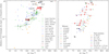 |
Fig. A.2 Same as Fig. A.1 but with α0 − αmin. |
| In the text | |
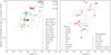 |
Fig. A.3 Same as Fig. A.1 but with 1 − αmin/α0. |
| In the text | |
Current usage metrics show cumulative count of Article Views (full-text article views including HTML views, PDF and ePub downloads, according to the available data) and Abstracts Views on Vision4Press platform.
Data correspond to usage on the plateform after 2015. The current usage metrics is available 48-96 hours after online publication and is updated daily on week days.
Initial download of the metrics may take a while.