| Issue |
A&A
Volume 683, March 2024
|
|
|---|---|---|
| Article Number | A123 | |
| Number of page(s) | 12 | |
| Section | The Sun and the Heliosphere | |
| DOI | https://doi.org/10.1051/0004-6361/202347799 | |
| Published online | 13 March 2024 | |
Spatially resolved radio signatures of electron beams in a coronal shock
1
Department of Physics, University of Helsinki, PO Box 64, 00014 Helsinki, Finland
e-mail: peijin.zhang@helsinki.fi
2
Heliophysics, NASA Goddard Space Flight Center, Greenbelt, MD 20771, USA
3
Department of Physics and Astronomy, University of Turku, 20500 Turku, Finland
Received:
25
August
2023
Accepted:
4
December
2023
Context. Type II radio bursts are a type of solar radio bursts associated with coronal shocks. Type II bursts usually exhibit fine structures in dynamic spectra that represent signatures of accelerated electron beams. So far, the sources of individual fine structures in type II bursts have not been spatially resolved in high-resolution low-frequency radio imaging.
Aims. The objective of this study is to resolve the radio sources of the herringbone bursts found in type II solar radio bursts and investigate the properties of the acceleration regions in coronal shocks.
Methods. We used low-frequency interferometric imaging observations from the Low Frequency Array to provide a spatially resolved analysis for three herringbone groups (A, B, and C) in a type II radio burst that occurred on 16 October 2015.
Results. The herringbones in groups A and C have a typical frequency drift direction and a propagation direction along the frequency. Their frequency drift rates correspond to those of type III bursts and previously studied herringbones. Group B has a more complex spatial distribution, with two distinct sources separated by 50 arcsec and no clear spatial propagation with frequency. One of the herringbones in group B was found to have an exceptionally large frequency drift rate.
Conclusions. The characteristics derived from imaging spectroscopy suggest that the studied herringbones originate from different processes. Herringbone groups A and C most likely originate from single-direction beam electrons, while group B may be explained by counterstreaming beam electrons.
Key words: methods: observational / Sun: activity / Sun: corona / Sun: radio radiation
© The Authors 2024
 Open Access article, published by EDP Sciences, under the terms of the Creative Commons Attribution License (https://creativecommons.org/licenses/by/4.0), which permits unrestricted use, distribution, and reproduction in any medium, provided the original work is properly cited.
This article is published in open access under the Subscribe to Open model. Subscribe to A&A to support open access publication.
1. Introduction
Low-frequency solar radio emissions are dominated by solar radio bursts that are classified into five main types (types I–V) based on their shape and dynamic spectrum characteristics. Type II solar radio bursts are characterized as slow frequency-drifting bursts toward lower frequencies, and they often exhibit complex structures in the dynamic spectra (e.g., Wild & McCready 1950; Mann et al. 1995; Cairns et al. 2003; Ramesh et al. 2023). Statistical and independent studies have shown that type II solar radio bursts are in general associated with coronal mass ejections (CMEs; Subramanian & Ebenezer 2006; Gopalswamy et al. 2019; Chen et al. 2014; Majumdar et al. 2021; Morosan et al. 2021; Kumari et al. 2023). In rare cases, type II bursts have been reported to occur in the absence of a CME. However, in these cases, the presence of a coronal shock wave can be inferred from multiwavelength observations (e.g., Su et al. 2015; Morosan et al. 2023).
Type II bursts are interpreted as the signature of shock-accelerated electron beams generating Langmuir waves close to the local plasma frequency (fp), and then converted into radio emission at the fundamental (F) and harmonic (H) frequency of fp (Nelson & Melrose 1985; Cairns et al. 2003). The volume emissivity of the plasma emission is strongly dependent on the plasma density distribution and the electron beams (Schmidt et al. 2014; Cairns et al. 2003; Kumari et al. 2017). As the shock can create complex plasma distributions around it (Hegedus et al. 2021), type II solar radio bursts usually have complex fine structures. One common fine structure in type II radio bursts is the herringbone structure (e.g., Cairns & Robinson 1987; Carley et al. 2013; Morosan et al. 2019, 2022), which manifests as a series of parallel lines in the dynamic spectra that resemble the pattern of a fish’s skeleton, hence the name. With the increasing resolution of the dynamic spectra provided by recent radio instruments, a wide variety of fine structures in type II radio bursts have been reported (Magdalenić et al. 2020).
Imaging spectroscopy of type II radio bursts can be used to locate shock-accelerated electron beams (e.g., Zucca et al. 2018; Morosan et al. 2019). With the new availability of low-frequency radio imaging, recent studies have provided improved multifrequency images of type II bursts and associated fine structures (e.g., Zucca et al. 2018; Morosan et al. 2019; Chrysaphi et al. 2020; Bhunia et al. 2023). For example, Zucca et al. (2018) used the tied-array beam observation mode (Morosan et al. 2014) of the Low Frequency Array (LOFAR; van Haarlem et al. 2013) on a type II solar radio burst. The observation was combined with a magnetohydrodynamic model of the solar corona to obtain the 3D source location. The results of the abovementioned study indicate that the type II burst is located at the CME flank where the shock proceeding direction is quasi-perpendicular to the background magnetic field. Morosan et al. (2019) also used tied-array beam imaging observations from LOFAR to image herringbone bursts and identified the presence of shock-accelerated electron beams at multiple regions around the CME shock. Maguire et al. (2021) used LOFAR interferometry imaging combined with extreme UV observations of a type II radio burst. They find that the radio source is located about 0.5 solar radii above a solar jet, which suggests the type II burst was generated by a jet-driven piston shock, instead of a CME-driven shock wave. In another study with the Murchison Widefield Array (MWA), Bhunia et al. (2023) performed radio imaging of a band-splitting type II event at multiple frequencies and found that the radio source is located at multiple locations close to the shock. Spatially resolved radiometry analysis is a powerful tool for analyzing the electron beam locations and propagation in detail, by imaging the fine structures in dynamic spectra.
In this paper we present the first high-spatial-resolution low-frequency study of the source of herringbone bursts. This paper is arranged as follows: in Sect. 2 we introduce the instrument and observation methods, including the imaging spectroscopy method and the data reduction procedure. Section 3 presents the type II radio burst event in the dynamic spectrum. Section 4 presents the interferometry observation of the herringbone structures in the type II radio burst. In Sect. 5 we analyze the observation results and compare them with previous studies. The overall conclusion is summarized in Sect. 5.
2. Observation and data reduction
We observed a type II radio burst with LOFAR’s low band antennas on 16 October 2015 in the frequency range 10–90 MHz. The observation mode used included imaging observations in interferometric mode and beam-formed observations with one beam pointed at the Sun to produce a dynamic spectrum. The dynamic spectrum measures the total flux from the target (the Sun), and the time and frequency resolution of the dynamic spectrum is 10.4 ms and 12.5 kHz. The dynamic spectrum is processed with ConvRFI (Zhang et al. 2023) to remove radio frequency interference.
The interferometric observation used 23 core stations and 12 remote stations. These 35 stations form 561 cross-correlation baselines in total. Two sub-array pointings were arranged to target the Sun and Virgo-A (calibrator source). For interferometric imaging, the integral time and frequency are 0.25 s and 195.3 kHz, respectively. The frequency channel spacing is, however, not uniform: in the range 20–58 MHz it is 195.3 kHz and in the range 58–80 MHz the spacing is 390.5 kHz. So far, this is the only LOFAR interferometric observation available with such a high-frequency resolution that allows us to study the evolution of low-bandwidth herringbones and other fine structures in type II bursts.
The type II burst on 16 October 2015, as shown in Fig. 1, is a fundamental-harmonic (F-H) pair event. The frequency ratio of the H- and F-components is 1.96 when comparing the bright part of each component. Band-splitting is visible in both F- and H- components. There are many complex structures in the harmonic lane, including herringbone bursts. We picked a few relatively isolated herringbone bursts in this type II event, labeled A, B, and C. We picked the herringbone structures that were most isolated from the background emission of the type II burst so that there is less confusion on the radio source identification of herringbones. For each individual herringbone, to get the frequency drift rate (FDR), df/dt, we performed a linear fit to the local maximum pixels in the herringbone lane. The fitting was applied to the reciprocal of the FDR dt/df (as df/dt can approach ±inf in this case). The uncertainty for each peak time pixel is the half-cadence (5.2 ms), which was taken into account to estimate the FDR uncertainty.
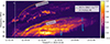 |
Fig. 1. Dynamic spectrum of the type II radio burst. The flux is normalized according to the quiet time flux (SB0), which represents the relative flux in reference to the quiet Sun. The fitted leading edge of the harmonic part of this type II is shown as solid green lines, and the solid orange line indicates the leading edge of the fundamental emission, derived from multiplying the radio of F/H = 1/1.96. Three herringbone groups are shown with blue boxes and labeled A, B, and C. The brightest time-frequency point is marked as a red triangle. |
The harmonic emission in the dynamic spectrum has a relatively distinct leading edge. We fitted the leading edge of the harmonic leading edge to f[MHz]=A(t − t0)B, where f is the frequency in MHz, t is the time offset in seconds, t0 is the launching time of the shock inferred from the leading edge, and the fitted value of t0 is 16 October 2015 12:52:41.717 UT. We also performed source kinematics analysis using interferometric images.
3. Results
This type II event features many complex structures in the harmonic lane, including numerous herringbone bursts. The three groups of herringbones selected, A, B, and C, are analyzed in detail below.
3.1. Herringbone group A
Sub-event A is a group of herringbones that occurred at 12:58:20 UT and around a frequency of 71 MHz. These herringbones have a reverse drift rate from low to high frequencies. The dynamic spectrum of this sub-event is shown in Fig. 2a. There are three herringbones, A1, A2, and A3. We obtained the local maxima points for each frequency channel in the dynamic spectrum to locate the herringbones. The marked local maxima points present the track of the herringbone in the frequency range of 69.3–70.9 MHz and 71.5–73.5 MHz (shown as blue plus symbols in the lower panel of Fig. 2a). There are also structures in the frequency range of 70.9–73.5 MHz that do not follow the frequency drift lane of the herringbone structure (local maxima shown as red symbols). However, the imaging of the excluded part (Fig. A.4) indicates that the source location is similar to herringbone group A. This source was not included in our imaging analysis since the drift rates do not match those of the selected herringbones and it may be a different burst.
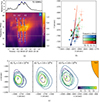 |
Fig. 2. Spectral characteristics and spatial location of herringbone group A. Panel a: dynamic spectrum of herringbone group A, consisting of three individual herringbone structures (A1, A2, and A3). The upper panel is the flux of 72.5 MHz (shown as a solid gray line in the dynamic spectrum), the blue plus sign marks the local maximum points along the herringbone, and the red plus marks the local maximum on the overlapped structures. The flux is in the relative unit in reference to the quiet time flux (SB0) before the burst time. The green line marks the frequency drift track of the herringbone. White rectangles mark the frequency and time integral span for the interferometric imaging. The upper panel is the flux slice through a frequency of 72.5 MHz (gray line in the lower panel). Panel b: source position of the herringbone structures in sub-event A. We used a Gaussian fit to determine the source location. The error bar indicates the location uncertainty. Three herringbone components (A1, A2, and A3) are presented in blue, green, and red. The brightness of the color represents the frequency. The arrow indicates the position variation with frequency, and the dashed lines connect each point in order of frequency. Panel c: interferometric imaging of the herringbone at different frequencies. Colored solid lines indicate the brightness temperature contour at 280 MK, and the plus sign marks the peak location of the brightness temperature distribution. The time and frequency slot is marked in panel a, and snapshot images are shown in Figs. A.1–A.3. |
By fitting the local maxima points of each herringbone component, we obtained the average frequency drift for each burst. The fitted values of dt/df (1/FDR) for A1, A2, and A3 are 0.1746 ± 0.0048 (MHz/s)−1, 0.044 ± 0.0071 (MHz/s)−1, and 0.0590 ± 0.0068 (MHz/s)−1, respectively. The corresponding FDRs of each herringbone are 5.7 MHz/s, 22.6 MHz/s, and 16.9 MHz/s, respectively.
Imaging of this herringbone group is done inside the time-frequency blocks marked in Fig. 2a, covering all local-maximum peak times for all available subbands. The width of each subband and the integral time of each time slot for imaging is indicated by the height and width of each weight block in Fig. 2a. The radio source shape and the location of each herringbone component are shown in Fig. 2c. The contour plot in this figure shows that the herringbones consist of a single source and have a simple geometrical shape.
The radio source locations show a frequency dependence that is demonstrated by a gradient-colored arrow, as shown in Fig. 2b. This outlines the frequency dispersion of herringbones. The herringbones trace a path from north to south for all three components (A1, A2, A3) and denote a common alignment of source location variation from high to low frequency. The starting and ending locations of the three tracks are separated by 20–50 arcsec. Considering the positive FDR, the temporal variation of the source is from north to south. Thus, the herringbones propagate southward in the plane of the sky. Some projection effects may, however, be present.
3.2. Herringbone group B
Group B occurs at 13:00:57 UT and around a frequency of 60 MHz. It consists of two herringbones, labeled B1 and B2, as shown in Fig. 3a. The two herringbones in this group are shown as blue plus symbols in the dynamic spectrum. By fitting the local maxima points of each herringbone component, we obtained the average FDR for each of these herringbones. Fitted value of dt/df (1/FDR) for B1 and B2 are − 0.0026 ± 0.0043 (MHz/s)−1, and 0.0634 ± 0.0071 (MHz/s)−1. The corresponding FDRs of each are −373.0 MHz/s and 15.7 MHz/s, respectively. B2 has a reverse frequency drift like the herringbones in group A; however, B1 appears almost vertical in the dynamic spectrum. The fitted value of 1/FDR is close to 0, and the error indicates the FDR can have values > 598 MHz/s or < −142 MHz/s. The frequency drifting direction is likely negative since the FDR corresponding to the center value of 1/FDR is −373 MHz.
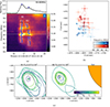 |
Fig. 3. Spectral characteristics and spatial location of herringbone group B. Panel a: dynamic spectrum of herringbone group B, consisting of two individual herringbone structures (B1 and B2). The upper panel is the 59.9 MHz flux (shown as a solid gray line in the dynamic spectrum), the blue plus sign marks the local maximum points along the herringbone, and the red plus sign marks the local maximum on the overlapped structures. The flux is in the relative unit in reference to the quiet time flux (SB0) before the burst time. The green line marks the frequency drift track of the herringbone. White rectangles mark the frequency and time integral span for the interferometric imaging. Panel b: source position of the herringbone structures in herringbone group B. We used a Gaussian fit to determine the source location. The error bar indicates the location uncertainty. Two herringbone components (B1 and B2) are presented in blue and red. The brightness of the color represents the frequency. The dashed lines connect each point in order of frequency. Panel c: interferometric imaging of the herringbone at different frequencies. Colored solid lines indicate the brightness temperature contour at 60 MK, and the plus sign marks the peak location of the brightness temperature distribution. The time and frequency slot is marked in Panel a, and snapshot images are shown in Figs. A.5 and A.6. |
Imaging of these herringbones shows complex spatial structures (see Fig. 3c). Additional detailed images at different frequencies are shown in Figs. A.5 and A.6. In some of the frequency subbands covering the imaging observations, we observe multiple peaks in intensity (e.g., < 60 MHz in Fig. A.6) that are combined to form a larger elongated radio source in these images. There are also frequency subbands with less complex features in radio images (e.g., > 62 MHz in Fig. A.6. To identify the herringbone source from multi-source images, we imaged the adjacent time-frequency point, as shown in Fig. A.7. During the time point inside the herringbone structure in the dynamic spectrum, there are two sources in images (upper and lower). However, outside the time point of the herringbone in the dynamic spectrum, the upper source disappears from the images. Therefore, the upper source most likely corresponds to the selected herringbone. Also, by comparing the multi-source images and the single-source images, the single sources appear to have well-aligned source sizes and positions with the upper west source in the multi-peak images. This source location also coincides with the time and frequency of the herringbones. Thus, the source location and dynamic analysis in this section are focused on the upper west source from the multi-source images.
The source location of the herringbones in this group is shown as centroids in Fig. 3b. The sources of the two components are not superposed as expected, instead, they are separated by 50 arcsec. The track traced by the radio sources with frequency is also not spatially aligned, unlike the herringbones in the first group (A1–A3). The source locations of B1 and B2 do not exhibit any clear dispersion in position with frequency, as expected from plasma emission. B1 shows a trend from west to east as frequency decreases from high to low, and the source of B2 shows a trend from east to west as frequency decreases from high to low.
3.3. Herringbone group C
The third group of the herringbone structure occurs around a frequency of 46 MHz and at 13:00:52 UT. This group has two herringbones labeled C1 and C2 that are temporally separated by 2.5 s. These herringbones have a forward drift from high to low frequencies. By fitting the local maxima points of each herringbone component to 1/FDR, we obtained the average frequency drift for each. The 1/FDR of C1 and C2 is −0.164 ± 0.045 and −0.268 ± 0.081, the corresponding FDR of each is −6.1 MHz/s and −3.7 MHz/s, respectively.
Imaging of this herringbone group is done inside the time-frequency blocks marked in Fig. 4a. The radio source’s shape and location of each component are shown in Fig. 4c. The contour indicates that the radio source of this event is a single source and relatively simple in spatial structure.
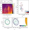 |
Fig. 4. Spectral characteristics and spatial location of herringbone group C. Panel a: dynamic spectrum of herringbone group C, consisting of two individual herringbone structures (C1 and C2). The upper panel is the 46.0 MHz flux (shown as a solid gray line in the dynamic spectrum), the blue plus sign marks the local maximum points along the herringbone, and the red plus sign marks the local maximum on the overlapped structures. The flux is in the relative unit in reference to the quiet time flux (SB0) before the burst time. The green line marks the frequency drift track of the herringbone. White rectangles mark the frequency and time integral span for the interferometric imaging. Panel b: source position of the herringbone structures in herringbone group C. We used Gaussian fitting to determine the source location. The error bar indicates the location uncertainty. Two herringbone components (C1 and C2) are presented in blue and red. The brightness of the color represents the frequency. The arrow indicates the position variation with frequency, and the dashed lines connect each point in order of frequency. Panel c: interferometric imaging of the herringbone at different frequencies. Colored solid lines indicate the brightness temperature contour at 200 MK, and the plus sign marks the peak location of the brightness temperature distribution. The time and frequency slot is marked in panel a, and snapshot images are shown in Figs. A.8 and A.9. |
The source centroids of this herringbone group are presented in Fig. 4b. The frequency trend of the centroids is indicated by the gradient-colored arrow. The track of these two components is spatially well aligned and shares the same position-frequency relation: from high to low frequency moving northward, opposite to the herringbones in group A. This confirms the theory that opposite drifting herringbones also propagate in opposite directions, as expected from the plasma emission mechanism (Melrose 1980). The electron beams producing the herringbones in groups A and C that move in opposite directions also confirm that bi-directional electron beams can escape the shock (Zlobec et al. 1993).
We also investigated some general properties of the herringbones in the three groups. Figure 5 shows the brightness temperature and source size of these three herringbone groups. The peak brightness temperature of these three groups ranges from 2 × 10⁷ K to 9 × 10⁸ K. Group A has the highest brightness temperature, while group B has the lowest brightness temperature. The size is measured in two ways: we estimated the 0.5 peak intensity radio source area as well as the extent in the x-direction, FWHMx. The 0.5 peak area represents the area of the region within the intensity contour of 0.5 times the peak TB for each herringbone. The FWHMx extent measures the full width of half maximum (FWHM) in the x direction over the radio source, obtained with the following procedure: first, we located coordinates of the upper source. Then, we plotted a slice in the x-direction from the peak and obtained the FWHM from that slice. The source area of group B has a significant variation at 59.5 MHz. The area at 58 MHz is ∼6–8 times larger than the area at 62 MHz in the same group. In this group, a frequency of 59.5 MHz marks the change between elongated and simple sources (see Figs. A.5 and A.6, where there are multiple sources and complex structures below 59.5 MHz, and the source structure is relatively single and clear for the source above 59.5 MHz). The FWHM in the x-direction for the three herringbone groups are all close to 4 arcmin. This indicates a source size significantly smaller than that of type III radio bursts (Kontar et al. 2019).
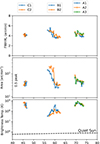 |
Fig. 5. Source size and brightness temperature of the herringbone structure. The area of the source is measured at half peak. |
Table 1 summarizes the frequency range, FDR, maximum brightness temperature, area, and FWHM size in the x direction. The obsolete value FDR of most of the traces are within the range of 3–30 MHz/s. Trace B1 has an exceptionally high FDR: −373.0 MHz/s. There is no apparent correlation between the FDR, frequency range, and brightness temperature.
Frequency range, FDR, and the brightness temperature of the source.
4. Discussion
Herringbone structures in type II solar radio bursts offer a unique diagnostic method for understanding the small-scale processes of electron kinematics close to the shock. The characteristics of the radio emission, combined with models and assumptions, can provide information on how electron beams are accelerated and escape the shock. The following are several conclusions that can be deduced from our observations.
4.1. Frequency drift rate
Assuming that one herringbone is generated by a single-direction electron beam, the FDR of the herringbone corresponds to the speed of the beam. The method of deriving the beam speed from FDR is often used in type III radio burst analysis (e.g., Zhang et al. 2018). Mel’nik et al. (2005) reported 1 MHz to 3 MHz FDR in the range of 10 MHz to 30 MHz for both positive and revert drift. Carley et al. (2015) reported  MHz for reverse drift and
  MHz for forward drifting herringbones in the range of 10–90 MHz. Based on previous observations (e.g., Carley et al. 2015; Cairns & Robinson 1987; Mann & Klassen 2005), the frequency drift direction stayed the same within the same group.
From our measurements of seven herringbones, the three herringbones in group A have positive drift, and the two in group C have negative drift. The drift rates of the herringbones from groups A and C are consistent with the results from Carley et al. (2015), Mann & Klassen (2005). The two herringbones in group B, however, have opposite frequency drift directions and B1 has an exceptionally large absolute value of the FDR. Using the coronal density model of Saito et al. (1977), and assuming the radio wave is generated by a single beam outward moving electron, we could derive the speed from the FDR. Usually, the speed of the beam electrons ranges from 0.1–0.6c, which corresponds to 6.3–38 MHz/s; for B1, on the other hand, 373 MHz/s corresponds to 5.92 times the speed of light, which is unphysical. There are two possible explanations for the exceptionally high FDR: (1) fast electron beams passing through a region with a drastic change in background plasma density and (2) multiple regions producing radio emission at different frequencies simultaneously. The second scenario can be achieved from multiple electron beams generating counterstreaming beam emission (Ganse et al. 2012).
4.2. Counterstreaming or single-direction beam electron
It is widely accepted that herringbones originate from electron beams that undergo acceleration by the CME shock (e.g., Cairns & Robinson 1987; Zlobec et al. 1993; Morosan et al. 2019). However, the specific mechanism behind this emission process remains uncertain with two possible ways of generating radio emission: (1) single-direction beam triggering Langmuir waves that are converted to radio waves through wave-wave interactions (Melrose 1980), similar to type III radio bursts and (2) counterstreaming electrons generate Langmuir waves, then the waves from the two beams interact and generate the radio waves (Knock et al. 2003; Ganse et al. 2012). In the latter, using particle-in-cell simulations (Ganse et al. 2012), radio emission can be detected in the case of counterstreaming beam electrons, while it is not detected in the single-direction electron beam scenario. This indicates that the requirement for generating radio waves is less strict for counterstreaming beam electrons. The possible emission mechanism is shown in the cartoon in Fig. 6, where a shock front (solid orange lines) propagates forward into quasi-perpendicular magnetic fields, creating multiple electron acceleration points (yellow stars). The accelerated electrons can move along the magnetic field without encountering other electrons, namely as single-direction electron beams, shown in the lower-left corner of Fig. 6. Some electron beams can encounter another stream of electrons moving in the antiparallel direction due to multiple shock ripple acceleration and reflection (Knock et al. 2003), namely the counterstreaming region, shown in the center part of Fig. 6.
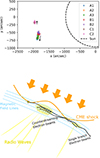 |
Fig. 6. Combined plot of the coordinates of the sources of the three herringbone groups (upper panel) and an illustrative cartoon model depicting the radio emission source of the herringbone structures (lower panel). |
These two types of electron beam distributions (single direction and counterstream) can have different spectroscopic features. The multiple bursts in a herringbone group from a single-direction electron beam should have similar source locations and moving directions aligned with the propagation direction of the radio sources. The FDR would also be similar to type III bursts. The herringbones generated by counterstreaming electrons would have arbitrary trajectories, as the encountering region could have different spatial distributions for each herringbone. The FDR is also likely to have extreme values as multiple electrons can contribute to the emission simultaneously and the encounter region is extended. Consequently, the sources from counterstreaming electrons are more likely to be extended, rather than point-like, as shown in Figs. A.5 and A.6. Thus, the B sources that could originate from counterstreaming electrons are more extended than A and C.
In our study, the sources in group A and group C have point-like sources, and the frequency-location track is aligned for all individual herringbone structures. This fits the scenario of the single-direction electron beams. Their FDR also has the same sign within the same group. Group B has extended sources and a relatively complex spatial structure, and an exceptionally high FDR for B1. B1 and B2 are also spatially separated, so these properties fit the counterstream electron beams theory better.
5. Conclusion
In this work we performed a detailed imaging spectroscopy analysis for herringbone bursts in a type II radio burst. Of the three herringbone structure groups studied, we find groups A and C have relatively simple imaging sources. For all three groups, the FDR has the same sign within the same group, and the FDR absolute values are similar to the type III bursts in the same frequency range. The imaging of group B shows that it has relatively complex spatial structures, and we observed multiple sources with extended structures in both the B1 and B2 subgroups; B1 has an exceptionally large FDR. Our observations suggest that groups A and C more likely originate from single-direction beam electrons, and group B is more likely generated from counterstreaming beams.
Acknowledgments
P.Z., D.E.M., and A.K. acknowledge the University of Helsinki Three-year Grant. D.E.M acknowledges the Academy of Finland project ‘RadioCME’ (grant number 333859). E.K.J.K. acknowledges the European Research Council (ERC) under the European Union’s Horizon 2020 Research and Innovation Programme Project SolMAG 724391 and the Academy of Finland Project 310445. The authors acknowledge the Finnish Computing Competence Infrastructure (FCCI) for supporting this project with computational and data storage resources and thank Discoverer Petascale Supercomputer (Sofia, Bulgaria) for the provided computing resources. A.K is supported by an appointment to the NASA Postdoctoral Program at the NASA Goddard Space Flight Center (GSFC). LOFAR (van Haarlem et al. 2013) is the Low Frequency Array designed and constructed by ASTRON. It has observing, data processing, and data storage facilities in several countries, which are owned by various parties (each with its own funding sources), and that are collectively operated by the ILT foundation under a joint scientific policy. The ILT resources have benefited from the following recent major funding sources: CNRS-INSU, Observatoire de Paris and Université Orléans, France; BMBF, MIWF-NRW, MPG, Germany; Science Foundation Ireland (SFI), Department of Business, Enterprise and Innovation (DBEI), Ireland; NWO, The Netherlands; The Science and Technology Facilities Council, UK; The Ministry of Science and Higher Education, Poland.
References
- Bhunia, S., Carley, E. P., Oberoi, D., & Gallagher, P. T. 2023, A&A, 670, A169 [NASA ADS] [CrossRef] [EDP Sciences] [Google Scholar]
- Cairns, I. H., & Robinson, R. D. 1987, Sol. Phys., 111, 365 [Google Scholar]
- Cairns, I. H., Knock, S. A., Robinson, P. A., & Kuncic, Z. 2003, Space Sci. Rev., 107, 27 [NASA ADS] [CrossRef] [Google Scholar]
- Carley, E. P., Long, D. M., Byrne, J. P., et al. 2013, Nat. Phys., 9, 811 [Google Scholar]
- Carley, E. P., Reid, H., Vilmer, N., & Gallagher, P. T. 2015, A&A, 581, A100 [NASA ADS] [CrossRef] [EDP Sciences] [Google Scholar]
- Chen, Y., Du, G., Feng, L., et al. 2014, ApJ, 787, 59 [NASA ADS] [CrossRef] [Google Scholar]
- Chrysaphi, N., Reid, H. A. S., & Kontar, E. P. 2020, ApJ, 893, 115 [NASA ADS] [CrossRef] [Google Scholar]
- Ganse, U., Kilian, P., Vainio, R., & Spanier, F. 2012, Sol. Phys., 280, 551 [NASA ADS] [CrossRef] [Google Scholar]
- Gopalswamy, N., Mäkelä, P., & Yashiro, S. 2019, Sun Geosphere, 14, 111 [NASA ADS] [Google Scholar]
- Hegedus, A. M., Manchester, W. B., & Kasper, J. C. 2021, ApJ, 922, 203 [NASA ADS] [CrossRef] [Google Scholar]
- Knock, S. A., Cairns, I. H., & Robinson, P. A. 2003, J. Geophys. Res. Space Phys., 108, 1361 [NASA ADS] [Google Scholar]
- Kontar, E. P., Chen, X., Chrysaphi, N., et al. 2019, ApJ, 884, 122 [NASA ADS] [CrossRef] [Google Scholar]
- Kumari, A., Ramesh, R., Kathiravan, C., & Wang, T. J. 2017, Sol. Phys., 292, 161 [NASA ADS] [CrossRef] [Google Scholar]
- Kumari, A., Morosan, D. E., Kilpua, E. K. J., & Daei, F. 2023, A&A, 675, A102 [NASA ADS] [CrossRef] [EDP Sciences] [Google Scholar]
- Magdalenić, J., Marqué, C., Fallows, R. A., et al. 2020, ApJ, 897, L15 [Google Scholar]
- Maguire, C. A., Carley, E. P., Zucca, P., Vilmer, N., & Gallagher, P. T. 2021, ApJ, 909, 2 [NASA ADS] [CrossRef] [Google Scholar]
- Majumdar, S., Tadepalli, S. P., Maity, S. S., et al. 2021, Sol. Phys., 296, 62 [NASA ADS] [CrossRef] [Google Scholar]
- Mann, G., & Klassen, A. 2005, A&A, 441, 319 [NASA ADS] [CrossRef] [EDP Sciences] [Google Scholar]
- Mann, G., Classen, T., & Aurass, H. 1995, A&A, 295, 775 [Google Scholar]
- Mel’nik, V. N., Konovalenko, A. A., Abranin, E., et al. 2005, Astron. Astrophys. Trans., 24, 391 [CrossRef] [Google Scholar]
- Melrose, D. B. 1980, Space Sci. Rev., 26, 3 [NASA ADS] [CrossRef] [Google Scholar]
- Morosan, D. E., Gallagher, P. T., Zucca, P., et al. 2014, A&A, 568, A67 [NASA ADS] [CrossRef] [EDP Sciences] [Google Scholar]
- Morosan, D. E., Carley, E. P., Hayes, L. A., et al. 2019, Nat. Astron., 3, 452 [Google Scholar]
- Morosan, D. E., Kumari, A., Kilpua, E. K. J., & Hamini, A. 2021, A&A, 647, L12 [NASA ADS] [CrossRef] [EDP Sciences] [Google Scholar]
- Morosan, D. E., Pomoell, J., Kumari, A., Vainio, R., & Kilpua, E. K. J. 2022, A&A, 668, A15 [NASA ADS] [CrossRef] [EDP Sciences] [Google Scholar]
- Morosan, D. E., Pomoell, J., Kumari, A., Kilpua, E. K. J., & Vainio, R. 2023, A&A, 675, A98 [NASA ADS] [CrossRef] [EDP Sciences] [Google Scholar]
- Nelson, G. J., & Melrose, D. B. 1985, in Solar Radiophysics: Studies of Emission from the Sun at Metre Wavelengths, eds. D. J. McLean, & N. R. Labrum, 333 [Google Scholar]
- Ramesh, R., Kathiravan, C., & Kumari, A. 2023, ApJ, 943, 43 [NASA ADS] [CrossRef] [Google Scholar]
- Saito, K., Poland, A. I., & Munro, R. H. 1977, Sol. Phys., 55, 121 [NASA ADS] [CrossRef] [Google Scholar]
- Schmidt, J. M., Cairns, I. H., & Lobzin, V. V. 2014, J. Geophys. Res. Space Phys., 119, 6042 [NASA ADS] [CrossRef] [Google Scholar]
- Su, W., Cheng, X., Ding, M. D., Chen, P. F., & Sun, J. Q. 2015, ApJ, 804, 88 [NASA ADS] [CrossRef] [Google Scholar]
- Subramanian, K. R., & Ebenezer, E. 2006, A&A, 451, 683 [NASA ADS] [CrossRef] [EDP Sciences] [Google Scholar]
- van Haarlem, M. P., Wise, M. W., Gunst, A., et al. 2013, A&A, 556, A2 [NASA ADS] [CrossRef] [EDP Sciences] [Google Scholar]
- Wild, J. P., & McCready, L. L. 1950, Aust. J. Sci. Res. Phys. Sci., 3, 387 [NASA ADS] [Google Scholar]
- Zhang, P., Wang, C. B., & Ye, L. 2018, A&A, 618, A165 [NASA ADS] [CrossRef] [EDP Sciences] [Google Scholar]
- Zhang, P., Offringa, A. R., Zucca, P., Kozarev, K., & Mancini, M. 2023, MNRAS, 521, 630 [NASA ADS] [CrossRef] [Google Scholar]
- Zlobec, P., Messerotti, M., Karlicky, M., & Urbarz, H. 1993, Sol. Phys., 144, 373 [Google Scholar]
- Zucca, P., Morosan, D. E., Rouillard, A. P., et al. 2018, A&A, 615, A89 [NASA ADS] [CrossRef] [EDP Sciences] [Google Scholar]
Appendix A: Imaging
Here we present interferometric imaging of the herringbone groups.
Group A:
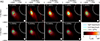 |
Fig. A.1. Interferometric imaging of herringbone fine structure A1. The beam shape of the cleaned beam is shown as a white circle in the lower-right corner of each panel. |
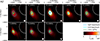 |
Fig. A.2. Interferometric imaging of herringbone fine structure A2. The beam shape of the cleaned beam is shown as a white circle in the lower-right corner of each panel. |
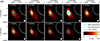 |
Fig. A.3. Interferometric imaging of herringbone fine structure A3. The beam shape of the cleaned beam is shown as a white circle in the lower-right corner of each panel. |
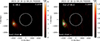 |
Fig. A.4. Comparison of source location for herringbone group A and the overlapped structure: within the herringbone (left) and outside the herringbone (right). |
Group B:
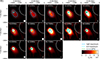 |
Fig. A.5. Interferometric imaging of herringbone fine structure B1. The beam shape of the cleaned beam is shown as a white circle in the lower-right corner of each panel. |
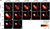 |
Fig. A.6. Interferometric imaging of herringbone fine structure B2. The beam shape of the cleaned beam is shown as a white circle in the lower-right corner of each panel. |
Adjacent time-frequency point imaging of B2:
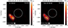 |
Fig. A.7. Imaging comparison of inside (left) and outside (right) herringbone structure B2. The left panel identical to the third panel of Fig A.6. The right panel is one time slot later than the left panel. |
Group C:
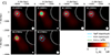 |
Fig. A.8. Interferometric imaging of herringbone fine structure C1. The beam shape of the cleaned beam is shown as a white circle in the lower-right corner of each panel. |
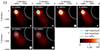 |
Fig. A.9. Interferometric imaging of herringbone fine structure C2. The beam shape of the cleaned beam is shown as a white circle in the lower-right corner of each panel. |
All Tables
All Figures
|
Fig. 1. Dynamic spectrum of the type II radio burst. The flux is normalized according to the quiet time flux (SB0), which represents the relative flux in reference to the quiet Sun. The fitted leading edge of the harmonic part of this type II is shown as solid green lines, and the solid orange line indicates the leading edge of the fundamental emission, derived from multiplying the radio of F/H = 1/1.96. Three herringbone groups are shown with blue boxes and labeled A, B, and C. The brightest time-frequency point is marked as a red triangle. |
| In the text | |
|
Fig. 2. Spectral characteristics and spatial location of herringbone group A. Panel a: dynamic spectrum of herringbone group A, consisting of three individual herringbone structures (A1, A2, and A3). The upper panel is the flux of 72.5 MHz (shown as a solid gray line in the dynamic spectrum), the blue plus sign marks the local maximum points along the herringbone, and the red plus marks the local maximum on the overlapped structures. The flux is in the relative unit in reference to the quiet time flux (SB0) before the burst time. The green line marks the frequency drift track of the herringbone. White rectangles mark the frequency and time integral span for the interferometric imaging. The upper panel is the flux slice through a frequency of 72.5 MHz (gray line in the lower panel). Panel b: source position of the herringbone structures in sub-event A. We used a Gaussian fit to determine the source location. The error bar indicates the location uncertainty. Three herringbone components (A1, A2, and A3) are presented in blue, green, and red. The brightness of the color represents the frequency. The arrow indicates the position variation with frequency, and the dashed lines connect each point in order of frequency. Panel c: interferometric imaging of the herringbone at different frequencies. Colored solid lines indicate the brightness temperature contour at 280 MK, and the plus sign marks the peak location of the brightness temperature distribution. The time and frequency slot is marked in panel a, and snapshot images are shown in Figs. A.1–A.3. |
| In the text | |
|
Fig. 3. Spectral characteristics and spatial location of herringbone group B. Panel a: dynamic spectrum of herringbone group B, consisting of two individual herringbone structures (B1 and B2). The upper panel is the 59.9 MHz flux (shown as a solid gray line in the dynamic spectrum), the blue plus sign marks the local maximum points along the herringbone, and the red plus sign marks the local maximum on the overlapped structures. The flux is in the relative unit in reference to the quiet time flux (SB0) before the burst time. The green line marks the frequency drift track of the herringbone. White rectangles mark the frequency and time integral span for the interferometric imaging. Panel b: source position of the herringbone structures in herringbone group B. We used a Gaussian fit to determine the source location. The error bar indicates the location uncertainty. Two herringbone components (B1 and B2) are presented in blue and red. The brightness of the color represents the frequency. The dashed lines connect each point in order of frequency. Panel c: interferometric imaging of the herringbone at different frequencies. Colored solid lines indicate the brightness temperature contour at 60 MK, and the plus sign marks the peak location of the brightness temperature distribution. The time and frequency slot is marked in Panel a, and snapshot images are shown in Figs. A.5 and A.6. |
| In the text | |
|
Fig. 4. Spectral characteristics and spatial location of herringbone group C. Panel a: dynamic spectrum of herringbone group C, consisting of two individual herringbone structures (C1 and C2). The upper panel is the 46.0 MHz flux (shown as a solid gray line in the dynamic spectrum), the blue plus sign marks the local maximum points along the herringbone, and the red plus sign marks the local maximum on the overlapped structures. The flux is in the relative unit in reference to the quiet time flux (SB0) before the burst time. The green line marks the frequency drift track of the herringbone. White rectangles mark the frequency and time integral span for the interferometric imaging. Panel b: source position of the herringbone structures in herringbone group C. We used Gaussian fitting to determine the source location. The error bar indicates the location uncertainty. Two herringbone components (C1 and C2) are presented in blue and red. The brightness of the color represents the frequency. The arrow indicates the position variation with frequency, and the dashed lines connect each point in order of frequency. Panel c: interferometric imaging of the herringbone at different frequencies. Colored solid lines indicate the brightness temperature contour at 200 MK, and the plus sign marks the peak location of the brightness temperature distribution. The time and frequency slot is marked in panel a, and snapshot images are shown in Figs. A.8 and A.9. |
| In the text | |
|
Fig. 5. Source size and brightness temperature of the herringbone structure. The area of the source is measured at half peak. |
| In the text | |
|
Fig. 6. Combined plot of the coordinates of the sources of the three herringbone groups (upper panel) and an illustrative cartoon model depicting the radio emission source of the herringbone structures (lower panel). |
| In the text | |
|
Fig. A.1. Interferometric imaging of herringbone fine structure A1. The beam shape of the cleaned beam is shown as a white circle in the lower-right corner of each panel. |
| In the text | |
|
Fig. A.2. Interferometric imaging of herringbone fine structure A2. The beam shape of the cleaned beam is shown as a white circle in the lower-right corner of each panel. |
| In the text | |
|
Fig. A.3. Interferometric imaging of herringbone fine structure A3. The beam shape of the cleaned beam is shown as a white circle in the lower-right corner of each panel. |
| In the text | |
|
Fig. A.4. Comparison of source location for herringbone group A and the overlapped structure: within the herringbone (left) and outside the herringbone (right). |
| In the text | |
|
Fig. A.5. Interferometric imaging of herringbone fine structure B1. The beam shape of the cleaned beam is shown as a white circle in the lower-right corner of each panel. |
| In the text | |
|
Fig. A.6. Interferometric imaging of herringbone fine structure B2. The beam shape of the cleaned beam is shown as a white circle in the lower-right corner of each panel. |
| In the text | |
|
Fig. A.7. Imaging comparison of inside (left) and outside (right) herringbone structure B2. The left panel identical to the third panel of Fig A.6. The right panel is one time slot later than the left panel. |
| In the text | |
|
Fig. A.8. Interferometric imaging of herringbone fine structure C1. The beam shape of the cleaned beam is shown as a white circle in the lower-right corner of each panel. |
| In the text | |
|
Fig. A.9. Interferometric imaging of herringbone fine structure C2. The beam shape of the cleaned beam is shown as a white circle in the lower-right corner of each panel. |
| In the text | |
Current usage metrics show cumulative count of Article Views (full-text article views including HTML views, PDF and ePub downloads, according to the available data) and Abstracts Views on Vision4Press platform.
Data correspond to usage on the plateform after 2015. The current usage metrics is available 48-96 hours after online publication and is updated daily on week days.
Initial download of the metrics may take a while.