| Issue |
A&A
Volume 685, May 2024
|
|
|---|---|---|
| Article Number | A107 | |
| Number of page(s) | 23 | |
| Section | Catalogs and data | |
| DOI | https://doi.org/10.1051/0004-6361/202346557 | |
| Published online | 14 May 2024 | |
Machine learning applications in studies of the physical properties of active galactic nuclei based on photometric observations★
DESY,
Platanenallee 6,
15738
Zeuthen, Germany
e-mail: sarah.mechbal@desy.de
Received:
27
March
2023
Accepted:
6
February
2024
Context. We investigate the physical nature of active galactic nuclei (AGNs) using machine learning (ML) tools.
Aims. We show that the redshift, z, bolometric luminosity, LBol, central mass of the supermassive black hole (SMBH), MBH, Eddington ratio, λEdd, and AGN class (obscured or unobscured) can be reconstructed through multi-wavelength photometric observations only.
Methods. We trained a random forest regressor (RFR) ML-model on 7616 spectroscopically observed AGNs from the SPIDERS-AGN survey, which had previously been cross-matched with soft X-ray observations (from ROSAT or XMM), WISE mid-infrared photometry, and optical photometry from SDSS ugriz filters. We built a catalog of 21 050 AGNs that were subsequently reconstructed with the trained RFR; for 9687 sources, we found archival redshift measurements. All AGNs were classified as either type 1 or type 2 using a random forest classifier (RFC) algorithm on a subset of known sources. All known photometric measurement uncertainties were incorporated via a simulation-based approach.
Results. We present the reconstructed catalog of 21 050 AGNs with redshifts ranging from 0 < z < 2.5. We determined z estimations for 11 363 new sources, with both accuracy and outlier rates within 2%. The distinction between type 1 or type 2 AGNs could be identified with respective efficiencies of 94% and 89%. The estimated obscuration level, a proxy for AGN classification, of all sources is given in the dataset. The LBol, MBH, and λEdd values are given for 21 050 new sources with their estimated error. These results have been made publicly available.
Conclusions. The release of this catalog will advance AGN studies by presenting key parameters of the accretion history of 6 dex in luminosity over a wide range of z. Similar applications of ML techniques using photometric data only will be essential in the future, with large datasets from eROSITA, JSWT, and the VRO poised to be released in the next decade.
Key words: accretion, accretion disks / methods: data analysis / catalogs / galaxies: active / galaxies: fundamental parameters / galaxies: photometry
A copy of the catalogue is available at the CDS via anonymous ftp to cdsarc.cds.unistra.fr (130.79.128.5) or via https://cdsarc.cds.unistra.fr/viz-bin/cat/J/A+A/685/A107
© The Authors 2024
 Open Access article, published by EDP Sciences, under the terms of the Creative Commons Attribution License (https://creativecommons.org/licenses/by/4.0), which permits unrestricted use, distribution, and reproduction in any medium, provided the original work is properly cited.
This article is published in open access under the Subscribe to Open model. Subscribe to A&A to support open access publication.
1 Introduction
Active galactic nuclei (AGNs) are known to be the most luminous sources in the Universe (Burbidge 1958; Minkowski 1960; Matthews & Sandage 1963; Schmidt 1963). These systems consist of a central supermassive black hole (SMBH), around which an accretion disk is formed (Lynden-Bell 1969; Rees 1984). Although much is yet to be learned about the feedback mechanisms linking SMBH growth and the evolution of their host galaxies (Ferrarese & Merritt 2000; Gebhardt et al. 2000; Yu & Tremaine 2002), we already know that their mass, MBH, scales with a number of galaxy properties, such as the stellar velocity dispersion, σ, bulge mass, and luminosity (see a review in Kormendy & Ho 2013). Furthermore, the extreme energetics of these objects also makes them a favored source of cosmic ray acceleration (Mannheim 1995; Halzen & Zas 1997; Murase 2022; Abbasi et al. 2022), as underlined by the recent discovery of neutrinos originating from the AGN NGC 1068 with IceCube (IceCube Collaboration 2022).
Collecting the physical parameters of SMBHs (e.g., red-shifts, z, black hole mass, MBH, and Eddington luminosity and ratio, LEdd and λEdd) from a complete and unbiased sample of AGNs stands as a necessary step in studying their accretion history (Sotan 1982; Magorrian et al. 1998; Schulze & Wisotzki 2010). However, spectroscopic techniques are almost always needed to measure these variables and although the number of spectroscopically observed AGNs has undoubtedly grown in the last decade (Plotkin et al. 2008; Kochanek et al. 2012; Menzel et al. 2016; Dwelly et al. 2017; Comparat et al. 2020), the discrepancy between photometrically identified AGNs and those followed up with spectroscopic surveys remains large (Blanton et al. 2017; Comparat et al. 2020). Fortunately, AGNs have been well covered by multi-wavelength surveys (Elvis et al. 1994; Edelson et al. 1996): X-ray telescopes have observed the extra-galactic sky (Brandt & Hasinger 2005), revealing a pattern of stars, black holes in binary systems, and AGNs, while infrared (IR) telescopes have allowed us to distinguish the latter from the large stellar population (Stern et al. 2005; Assef et al. 2013).
Enlarging the sample and sky coverage of AGN observations with reliably estimated physical parameters is particularly important for multimessenger astronomy, where signals from individual sources are often weak (Aartsen et al. 2020; Abbasi et al. 2023). This limitation can be overcome by searching for correlations between a messenger (e.g., neutrinos or cosmic rays) and a population of AGNs instead. However, the power of correlation searches increases with the sky coverage of the counterpart observations and, additionally, this requires a model for the expected production of the messenger in question for each object included in the correlation study (Achterberg et al. 2006; Aartsen et al. 2017; Abbasi et al. 2022). Such models usually depend on the physical parameters of the specific AGN.
Machine learning (ML) techniques have been applied in recent years to characterize AGNs and galaxies in general, for classification tasks, redshift determinations (Cunha & Humphrey 2022; Dainotti et al. 2021; Fotopoulou & Paltani 2018; Sadeh et al. 2016), and reconstructions of their physical properties. Li et al. (2021), Clarke et al. (2020), Fotopoulou & Paltani (2018), and Khramtsov et al. (2020) all trained ML classifiers using multi-wavelength photometric datasets to distinguish galaxies, quasars, and stars from one another. While Ucci et al. (2017); Rhea et al. (2021) used spectral measurements of galaxies and ML algorithms to infer the physical properties of the host galaxies, Bonjean et al. (2019) and Simet et al. (2021) used photometric measurements only and ML regression to determine star formation rates, while the M*, parameters have usually been reconstructed from spectroscopy observations or template fitting methods. We follow this latter approach in this paper.
We report on a novel attempt to employ ML regression tasks to reconstruct the fundamental parameters of AGNs. We trained a ML algorithm to estimate z, Lx, and LBol, along with the soft X-ray (SXR) and bolometric luminosities, as well as MBH, LEdd, and λEdd on 21 050 AGNs, all observed in the IR, optical, and X-ray bands photometrically – but not spectroscopically. To train the model, we used the recent SPIDERS-AGN spectroscopic survey (Clerc et al. 2016; Dwelly et al. 2017), which has compiled and released a sample of ~7600 type 1 AGNs (Coffey et al. 2019). In addition, we also trained a ML classifier to identify type 2 (or obscured) from type 1 (unobscured) AGNs.
The structure of the paper is as follows: we detail the catalogs used to expand and build both the AGN training sample and the data sample that is to be reconstructed in Sect. 2 and we describe the procedures to select AGNs from stellar, galactic, and blazar populations. We detail in Sect. 3 how the errors on the input parameters have been incorporated to generate pseudo-sets for the classification, training, and reconstruction of AGNs, and underline the advantages of the simulation-based method, before classifying the unlabeled sources using ML tools in Sect. 4. In Sect. 5, we describe the details of the main ML regression task built to parametrize the core of AGNs. We also discuss our comparison of several models and the final results from the spectroscopic parameter predictions. In Sect. 6, we present in the largest catalog (to date) of AGN physical properties, stemming from the ML reconstruction of 21 050 sources, including 11 363 new z measurements, and LBol, MBH, and λEdd values for all. The limits of the type 2 AGN reconstruction are also discussed. We turn to future prospects following the release of this dataset in Sect. 7 and discuss the role ML tools will play with the advent of future missions. The catalog columns are described in Appendix A.
Catalogues and their references used to build the multiwavelength inputs to the machine learning algorithm.
2 Data
Here, we provide a high-level summary of the different datasets used to build the reconstructed catalog and augment the training dataset. A detailed account of the multiwavelength observations used is given in Sects. 2.1–2.5. Table 1 summarizes all input features used for the training and reconstruction of the ML regressor, along with their catalog of origin. The analysis sequence to create the full reconstructed catalog is described in Fig. 1. The target parameters for the ML regression are presented in Table 2.
The starting point for building the reconstructed catalog is the 2RXS/XMMSL2-AllWISE dataset released in Salvato et al. (2018). Those 123 436 AGNs have been soft X-ray- and infrared-selected and already cross-matched, using the 2RXS (Boller et al. 2016) and XMMSL22 catalogs from ROSAT (0.1–2.4 keV) and XMM-Newton (0.2–12 keV) for X-ray flux and error, respectively. In the infrared, the AllWISE catalog (Cutri et al. 2021) provided observations at 3.4, 4.6, 12 and 22 μm (W1, W2, W3, and W4 bands, respectively), with their respective errors. Cuts are performed on the X-ray flux, and the IR color-color bands to remove non-AGN sources, leaving 60 888 sources (see Sect. 2.5). For optical photometry and spectroscopy information, we cross-matched the remaining sources with data from the Sloan Digital Sky Survey (SDSS): 21 050 sources were found to have been photometrically observed in the instrument specific ugriz (3543–9134 Å) filters (Lyke et al. 2020), while a subset of 9944 sources were also observed spectroscopically (380–920 nm band): for these, the redshift, z, and the classification CLASS_BEST were recorded, and 195 sources classified by SDSS as blazars, BL Lacertae (BLLACs), or stars were removed. We required for all sources to have SDSS photometry observations. Gaia DR1 catalog (Arenou et al. 2017) was also cross-matched in Salvato et al. (2018): the white-light G-band (330-1050 nm) mean flux and mean flux error was also recorded for 14 887 cross-matched sources, expressed in photo-electrons s−1. For the remaining 6097 without Gaia observations, we handled the null entries by creating synthetic values of the flux and error. The same method was applied to fill 21, 89, 1931 and 7156 missing W1, W2, W3, and W4 error entries. This was done for features found to have a minimal importance in the regression task, while aiming to maximize the number of sources in the catalog, to avoid the indiscriminate removal of any point with a missing parameter. Appendix C describes the handling of null entries and its effect on the reconstruction in more detail.
For the training dataset, we used 7616 type 1 AGN sources from the SPIDERS-AGN catalog (Coffey et al. 2019), a completed SDSS-IV spectroscopic survey. All AGNs that were all observed photometrically in the X-ray, IR, and optical bands prior to the survey, and the input catalog was augmented with the datasets listed above. The released dataset gives key AGN parameters derived from the spectral lines: redshift, z, bolometric luminosity, LBol, black hole mass estimate, MBH, and Eddington ratio, λEdd. These variables constitute the target parameters for the ML regression.
For matters pertaining to machine learning methods, a few terms also need be clearly defined:
by training and testing sample, we mean the dataset of 7616 sources built from the SPIDERS catalog used to train the ML model tasked to learn the correlations between photometric and spectroscopic parameters. The performance of the ML model is assessed by comparing the true and predicted values of target parameters (also referred in the ML literature as the “validation” set),
we refer to the AGN catalog we built for as the call the “reconstructed” or “full” dataset, which we used to make estimations on the target parameters using the previously trained ML model.
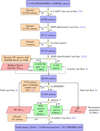 |
Fig. 1 Flowchart of the analysis. The starting point 2RXS/XMMSL2-A11WISE catalog released in Salvato et al. (2018), leading to the catalog of 21 050 reconstructed AGN sources presented in this work. |
Target variables, their domain range and error estimate from the SPIDERS catalogue (Coffey et al. 2019).
2.1 The SPIDERS-AGN catalog
SPectroscopic IDentification of ERosita Sources (SPIDERS) is a completed SDSS-IV (Blanton et al. 2017) 5128.9 deg2 survey over the SDSS footprint. The AGN sources were originally pre-selected based on the 1RXS and XMMSL1 (Saxton et al. 2008) catalogs, which were then later updated once the 2RXS (Boller et al. 2016) and XMMSL2 were released. The details of the mission targeting and summary are documented in Dwelly et al. (2017) and Comparat et al. (2020), respectively. The spectroscopic data was made available in the 16th SDSS data release (DR16; Ahumada et al. 2020) as a catalog of type 1 AGNs containing X-ray fluxes, optical spectral and photometric measurements, black hole estimates, and other derived quantities3. We refer the reader to Coffey et al. (2019) for a detailed description of the dataset and to Wolf et al. (2020) for a principal component analysis (PCA) of type 1 AGN properties.
The survey probed the brightest X-ray sources in the sky, at the higher end of the luminosity distribution with 41 < log10(LX/ergs−1) < 46 for a mean redshift  . The bolomet-ric luminosity, LBol, was also derived from the monochromatic luminosity, L3000 Å and L5100Å, using bolometric corrections. Fitting the Hβ and MgII emission lines, the SPIDERS-AGN study derived the MBH,
  , and λEdd = LBol/LEdd, with M⊙ being the solar mass. For 2337 sources, both the Hβ and MgII lines were observed, and two estimates of MBH and derived quantities were provided: in such cases, we selected the values with the smallest associated error
  , which has a typical value of ~ 0.02 dex. Table 2 presents a list of the key properties found in the SPIDERS-AGN catalog, with their respective range and median estimate error. Out of 7670 AGNs, there are 7616 with complete spectroscopic information, which we used as the basis of our training sample and we expanded on it using several other astronomical catalogs.
2.2 X-ray data
X-ray band observations are some of the most effective data samples for identifying AGNs: emission is believed to come from above the accretion disk; from there, photon scatter onto the hot corona gas and emit X-rays via inverse Compton. Although binary systems such as accreting neutron stars and stellar-mass black holes are also X-ray emitters, AGNs are generally more luminous by an order of magnitude (LX > 1042 erg s−1) (Hickox & Alexander 2018).
The ROSAT telescope (Trümper 1982) performed the first all-sky survey (RASS) between 1990 and 1991 in the 0.1–2.4 keV band. Two catalogs, one for faint and another for bright sources, were then released (Voges et al. 2000). The data were reprocessed decades later, leading to a second data release, the 2RXS catalog, comprising ~135 000 sources (Boller et al. 2016). XMMSL2 is the second catalog of X-ray sources found in slew data taken by the XMM-Newton European Photon Imaging Camera pn (EPIC-pn) in three bands: 0.2–12 keV (B8), 0.2–2 keV (B7), and 2–12 keV (B6). The B8 band is the most complete and the one of interest. The starting point of our reconstructed catalog building is the work of Salvato et al. (2018): 106 573 X-ray sources from 2RXS and 17665 sources from XMMSL2 (with | b | > 15°) were cross-matched with their All-WISE (Wright et al. 2010) and Gaia (Gaia Collaboration 2018) counterparts using a newly developed Bayesian algorithm to overcome the large positional uncertainties of the X-ray observations. Two catalogs were subsequently released: 2RXS-AllWISE and XMMSL2-AllWISE4.
To combine the two X-ray datasets, several steps must be taken to match the different response functions and detection range of the instruments. We first converted the ROSAT fluxes from the original 0.1-2.4 keV into the classical soft X-ray band 0.5-2 keV (Dwelly et al. 2017) as follows:
![${{F\left[ {E_{\max }^\prime :E_{\min }^\prime } \right]} \over {F\left[ {{E_{\max }}:{E_{\min }}} \right]}} = {{E_{\max }^{2 - {\rm{\Gamma }}} - E_{\min }^{\prime 2 - {\rm{\Gamma }}}} \over {E_{\max }^{2 - {\rm{\Gamma }}} - E_{\min }^{2 - {\rm{\Gamma }}}}},$](/articles/aa/full_html/2024/05/aa46557-23/aa46557-23-eq4.png) (1)
(1)
where Γ = 1.7 for 2RXS sources.
In Dwelly et al. (2017), Γ = 2.4 was chosen for XMMSL2 fluxes: however, the 2RXS/XMMSL2 datasets were kept separate. About a thousand sources from the SPIDERS AGN catalog have been observed with both instruments: we use these as a control group for matching the XMM to the converted RXS fluxes, by varying the Γ power-law index of Eq. (1) in order to match the peaks of the two X-ray flux distributions (as shown in Fig. 2). Choosing ΓΧΜΜ=1.25, 94% of sources present in both datasets have a flux ratio  within 5% of one another. In the converted SRX band, the distribution of X-ray fluxes is contained between 10−14 < F0.5–2keV < 10−9 erg cm−2s−1. From the X-ray catalogs, we only kept the X-ray fluxes and corresponding errors in the converted 0.5–2 keV band as input to the ML-model. Whereas the hardness ratio and/or column density would have offered valuable information on the class of AGNs, both being a known proxy for the obscuration level of accretion disks, this parameter was neither complete, nor very accurate, in the case of ROSAT observations; thus, it had to be dropped.
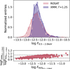 |
Fig. 2 Top: 2RXS and XMMSL2 fluxes for the ~1000 SPIDERS-AGN sources observed with both instruments. The X-ray fluxes were converted to the soft X-ray band 0.5−2.0 keV using Γ=1.7 for 2RXS and Γ=1.25 for XMMSL2, value chosen to match the peaks of the two distributions. Bottom: ratio of the converted flux logs as a function of the 2RXS fluxes for the same sources shown in the above panel. The dashed lines represent the ±5% level on the ratio, within which 94% of the converted fluxes are. |
2.3 Infrared observations
In the mid-infrared (MIR, 3–30 μm), AGNs are bright. The dusty torus is responsible for this thermal emission, as it absorbs shorter-wavelength photons from the accretion disk and re-emits them in the MIR. Although star-forming galaxies are also bright in this band, their SED is cooler and can be distinguished from those of AGNs (Padovani et al. 2017). The Wide-field Infrared Survey Explorer (WISE; Wright et al. 2010) is a satellite launched in 2009. The missions was then later extended under a new appellation, NEOWISE (Mainzer et al. 2011). The combination of WISE and NEOWISE data was made available to the public with the release of the AllWISE catalog (Cutri et al. 2021). The WISE survey scanned the sky at 3.4, 4.6, 12, and 22 μm (the bands designated as W1, W2, W3, and W4, respectively), at a depth at which the majority of the resolved 2RXS and XMMSL2 populations are to be detected (Salvato et al. 2018). In addition to the 4 MIR magnitudes and their associated errors, we explicitly record the relative magnitudes W1–W2, W2–W3, and W3–W4. These values are readily available from Salvato et al. (2018), as previously mentioned.
2.4 Optical data
2.4.1 Photometry
SDSS. The Sloan Digital Sky Survey (SDSS) has in the course of its runs observed over 700 000 quasars in the optical band, most of them in broadband photometry in the instrument specific ugriz (3543–9134 Å) filters (Lyke et al. 2020). To pair the AGN sources from our training and unknown sets with their SDSS observations, the astroquery software tool (Ginsburg et al. 2019) was used: we cross-matched the best AllWISE counterpart to the X-ray sources in our training and reconstructed samples with an optical counterpart from the DR17 photometric catalog, setting a maximum radius of 5 arcsec. For the matched sources, we add as features the SDSS PSF magnitudes psfMag and their associated error psfMagErr for the five ugriz bands. These values are most appropriate when studying the photometry of distant quasars. Logically, all 7616 SPIDERS sources have SDSS photometry counterparts, however, 47739 (5985) 2RXS (XMMSL2) sources have been observed photometrically, which we added as a requirement (see Fig. 1).
Gaia. Salvato et al. (2018) also cross-matched the 2RXS/XMMSL2 sources to the first release catalog of the Gaia mission (Arenou et al. 2017). The astrometric instrument performs broadband photometry in Gaia’s white-light G-band (330–1050 nm): we kept the mean flux and mean flux error for all sources, expressed in photo-electrons s−1.
2.4.2 Spectroscopy and redshift
Prior to the start of the SPIDERS mission, X-ray+AllWISE AGN targets were cross-matched with the already observed SDSS I—II–III runs (Dwelly et al. 2017): ~12 000 ROSAT and ~1500 XMM–Newton sources were found to already have been observed with spectroscopy. After performing a visual inspection of the optical spectra, two value-added catalogs (VAC) were released5. These included redshift measurements, along with object main and sub-classifications. Matching sources from the reconstructed catalog by their X-ray name, we found 21 287 (2540) 2RXS (XMMSL2) sources previously observed spectro-scopically: of these, 11 242 (1250) contain redshift information (but no black hole mass or Eddington ratio). As we explain in Sect. 5.3, this latter variable greatly improves the ML predictions. Furthermore, we will make use of the sub-sample of sources for which we have an AGN classification to correlate multiwavelength observations with the AGN obscuration level (see Sect. 4). Following the classification scheme of Comparat et al. (2020), we mark AGNs as either type 16 or 27, following the SDSS pipeline automated classification (Bolton et al. 2012).
Additional spectroscopic classification and redshift measurements are found in the VERONCAT catalog (Véron-Cetty & Véron 2010), a collection of some ~150 000 quasars from multiple surveys. The X-ray positions of sources were then cross-matched with the optical or radio positions given by VERON-CAT, using a maximum matching radius of 60 arcsec, a value taken from a past study (Abbasi et al. 2022). This allowed us to get additional AGN classification and spectral class features. We collected some ~9000 redshifts from VERONCAT, in addition to those already found from previous SDSS surveys. To verify the accuracy of the cross-matching, we compare the red-shift entries from the 6163 SPIDERS sources that are already present in VERONCAT, Δz =| zSPIDERS – zVERONCAT |. We found that 98% of the sources have Δz < 0.01, confirming the adequacy of the cross-matching radius used.
2.5 AGN selection
The multiwavelength data collected in the previous sections can then be used to select AGNs from a larger sample comprising of blazars, galaxies, and stars using X-ray and IR colors observations. Following the source characterization methods already established in Salvato et al. (2018) and the references therein, we proceeded to a first selection of AGNs in the X-ray/MIR plane (see top panel of Fig. 3). An empirical relationship was found, separating AGNs from stars and galaxies.

We can confirm the validity of such a selection by overlaying the confirmed AGNs in the SPIDERS sample, which all clearly lie above the cut-off line. We then use the AllWISE W1–W2, W2–W3, and W3–W4 relative magnitudes to isolate AGNs from blazars and starbust and normal galaxies, as developed in Assef et al. (2013). In the W1–W2 versus W2–W3 digram (middle panel of Fig. 3), the stars and elliptical galaxies exhibit colors near zero and are located in the lower left quadrant, while the spiral galaxies are red in W2–W3, but not in W1–W2, and ultra-luminous infrared galaxies (ULIRGS) are red in both, lying in the upper right quadrant of the diagram (Wright et al. 2010). We selected the sources for which 1.5 < W2–W3 < 4.5 and 0.2 < W1–W2 < 1.75 (black square in middle panel of Fig. 3). Once again, we used the SPIDERS AGN sample to justify the selection criteria being made in the W1–W2 versus W2–W3 color-color space. Similarly, a visual cut was made on the W1–W2 vs. W3–W4 plane, following the SPIDERS-AGN locus (black line of bottom panel in Fig. 3) (Abbasi et al. 2022).
After these selections, 60 952 AGN are identified, from an original sample of 123 436 X-ray-AllWISE sources. The spatial distribution of the final catalogue is shown in Fig. 4: the sources follow the SDSS footprint, as the requirement to have been observed photometrically by SDSS marks the most stringent cut on the data.
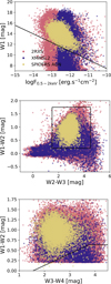 |
Fig. 3 Top: distribution of sources in the W1 band vs. soft X-ray flux parameter space for the ALLWISE counterparts to 2RXS (pink) and XMMSL2 (blue). The confirmed SPIDERS AGN are represented in yellow. The cut defined in Eq. (2) is also shown. W1–W2 magnitude plotted against the W2–W3 (middle) and W3–W4 (bottom). The black lines show the cuts applied based on the SPIDERS AGN position. |
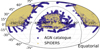 |
Fig. 4 Spatial distribution of sources in equatorial Mollweide projection for the for the selected AGN sample (in blue) and the SPIDERS AGN sample (yellow). The requirement for all sources to have been observed by SDSS constrain their distribution to the Northern Sky footprint. The galactic plane is shown as a gray line. |
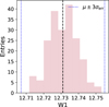 |
Fig. 5 Distribution of W1 input smeared by the measurement uncertainty for a single source. Each point is drawn from a normal distribution centered at the given catalogue input feature μvalue (black dashed line) and extending to ±3σerr. (blue dotted lines), from the given photometric measurement error. |
3 Measurement uncertainties and pseudo-sets
Each photometric observation used as an input (presented in Table 1) comes with a measurement uncertainty of non-constant variance (also called “heteroscedastic” error). Properly taking them into account is an active area of study in astrostatistics (Feigelson et al. 2021). Considering the stochastic nature of both input features and ML models, we adopted the approach outlined in Shy et al. (2022): all measurement errors, σerr, are assumed to be Gaussian, so that any photometric input for a single source is represented as a normal distribution, centered around the given value μvalue, extending to ±3σerr. Figure 5 shows such an example of the W1 for a single training source with the measurement given by μvalue (black dashed line) and μvalue ± 3σerr (blue dotted lines).
Drawing randomly from each independent “smeared” input distributions, we can thus create N pseudo-sets for each AGN source, where the photometric inputs differ within ±σerr between each realization. We create N = 200 pseudo-sets of both the training (for the regression) and the reconstructed datasets. The given photometric errors are not added as explicit features of the ML training, but are included through the scatter present in the photometric features across the N pseudo-sets. Sections 4 and 5 further develop the way this simulation-based treatment of measurement errors helps characterize both the performance and reconstruction of unlabeled or unknown data in the context of ML classification and regression tasks.
4 Machine learning classifier for type 2 AGN identification
Once the AGNs have been identified, a further step is needed, namely: since our training sample exclusively contains type 1 AGNs (broad emission line, unobscured), we must distinguish type 1 from type 2 (narrow emission line, obscured) in our reconstructed sample to study any potential biases in the spectroscopic predictions. Obscured AGNs (also called type 2) are systems where the emission from the accretion disk gets absorbed and scattered by dust or gas surrounding it, masking some of the characteristic signature of the AGN: the AGN unification model (Antonucci 1993; Urry & Padovani 1995) states that the obscuration effect is merely a by-product of the observer’s orientation, while others (Laor 2003; Elitzur & Shlosman 2006; Ricci et al. 2011) claim there to be a structural difference in the narrow- and broadline regions of AGNs.
The impact of such a suppression is wavelength-dependent, and a reliable and complete identification method of this population remains challenging and important. Distinctions between type 1 and type 2 AGNs can be made across multiple photometric and spectroscopic observation types. For a review on obscured AGNs, we refer to Hickox & Alexander (2018). The most classical way to identify an AGN class is through UV-NIR spectroscopy (Comparat et al. 2020; Koss et al. 2022). Type 1 AGNs have broad emission lines showing velocity dispersion > 1000 km s−1, while type 2 AGNs have narrow emission lines only, with a velocity dispersion <1000 km s−1 (Padovani et al. 2017). However, since the purpose of this study is to characterize AGNs that have not been spectroscopically observed, we must circumvent the absence of such of information.
Our sources were originally selected based on their soft X-ray flux (Salvato et al. 2011): this already skews the sample towards a majority of type 1 sources, as soft X-rays get absorbed by the high hydrogen column density, NH, around the accretion disk (Hasinger 2008), while harder X-ray are less suppressed in obscured AGNs (Ananna et al. 2022). These are also known to have stronger emission in the MIR than they do in other bands, as larger dust column reprocesses radiation from other bands. We thus expect weak UV/optical/NIR emission compared to that of the MIR (Hickox & Alexander 2018). As described in Sect. 2.4.2, we already know the AGN class for a sub-sample of sources that have a classification CLASS_BEST, so that the correlations between photometric observations and the object type can be studied. One could try to identify a single feature that best allows the distinction between obscured and unobscured AGNs, such as the ratio of W2/W1 IR emission. We developed this “classical” method following the method used in Abbasi et al. (2022) and detailed in in Appendix B. However, a more judicious use of the multiwavelength information collected would be to train a classification machine learning model. Taking the 13 415 sources for which SDSS classification is known as a training sample, we add a new feature called “obscuration”: its value is 0 for type 1 AGNs and 1 for type 2 AGNs. We followed the classification into type 1 or 2 employed in the SDSS pipeline, whereby spectral templates to distinguish between the classes (Bolton et al. 2012). We then sought to characterize whether the remaining 15 533 are obscured or not.
4.1 Imbalanced classification
Of the 13 415 labeled sources, 12 629 are unobscured (including SPIDERS sources which are all type 1), while 786 are obscured AGNs, a ratio of 16:1. This classification task is thus an imbalanced one; this is a frequent situation, where a classifier must learn to identify a minority case, although it is trained on a dataset over-represented by a majority case. This ultimately leads to bias in the reconstructed sample.
Many strategies exist to mitigate this issue (Barandela et al. 2003; Batista et al. 2004; Wang et al. 2021; Kim &Hwang 2022). One approach is to randomly resample the training dataset: we can perform either a random undersampling (RUS) of the majority caused by selecting a sub-sample of type 1 AGNs or a random oversampling (ROS), where points in the minority class are duplicated. In both cases this results in a changed n1/n2 ratio, brought closer to parity. Both methods present some disadvantages: in the case of RUS, the greater part of the majority class is discarded and lost to the model training, while in ROS, the naive duplication of minority samples can lead to overfitting. One can also perform a more sophisticated type of oversampling, via SMOTE (Synthetic Minority Oversampling Technique), where k-nearest neighbors are found to create synthetic minority class points (Chawla et al. 2002).
We tested baseline (no mitigation strategy), undersampling, oversampling, and SMOTE methods by training a random forest classifier (RFC; Breiman 2001) with 18 smeared photometric measurement as input features (see Sect. 3). We used a stratified five-fold cross-validation method (Stone 1974) to separate the training and testing sets, ensuring that all points were used for training and validation at least once. The resampling of the data was applied to the training datasets only, while the testing set retained the original imbalance of our AGN catalog.
We call a true positive (TP) a type 2 AGNs classified as type 2, a false positive (FP) a type 1 classified as type 2, a true negative (TN) a type 1 classified as type 1, and a false negative (FN) a type 2 classified as type 1. The precision of the classification is then defined as:
 (3)
(3)
that is, the ability of the classifier not to label as positive a sample that is negative. The recall, also called sensitivity or true positive rate (TPR), is calculated with:
 (4)
(4)
that is, the ability of the classifier to find all the positive samples. For completion, we provide the definition of the false positive rate (FPR), used in the receiving operating characteristic (ROC) curve8,
 (5)
(5)
so that it is a measure of finding all the negative samples.
Figure 6 shows the confusion matrices for all tested resampling method presented in Fig. 6. As expected, the baseline model, while it is able to identify type 1 AGNs with ease (99% TPR), it is not able to reliably identify type 2 AGNs. The same can be said of the ROS, where the naive duplication of minority samples seems to improve the classification only slightly. Clear improvements start to show for the RUS and SMOTE trained samples. The RUS method shows a larger type 2 AGNs recall than the SMOTE technique (90% vs. 80%), but a decreased precision, with a larger fraction of type 1 AGNs falsely identified as type 2 AGNs (12% for RUS, 5% for SMOTE). Using SMOTE to train the RF classifier thus appears to be a good compromise between precision and recall, with a larger fraction of properly classified type 1 AGNs (the greater dataset), along with an acceptable identification of type 2 AGNs.
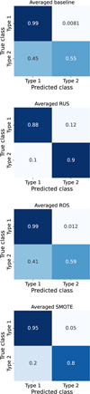 |
Fig. 6 Confusion matrices for different imbalanced classification mitigation techniques. The naturally imbalanced set (baseline), while accurately selecting Type 1 AGN 99% of the time, performs poorly in finding the rarer Type 2 AGN. Both RUS and SMOTE techniques show great classification improvements. |
4.2 Classification accuracy on the labeled set
After the study on a single pseudo-set, we settled on training a random forest classifier using the SMOTE method. To propagate the photometric measurement uncertainties in the input features, we made use of the N = 200 pseudo-sets previously generated (see Sect. 3) to label the unknown AGNs. We follow the steps outlined in Shy et al. (2022): for each simulation set, a classifier is fit to a realization of the labeled data, then used to reconstruct a realization of the unlabeled data. This way, all sources are reconstructed N times, whether they belong to the unlabeled or the validation datasets. For all performance metrics defined in Sect. 4.1, we thus obtained a posterior predictive distribution comprising of the results of each set’s classification (Fig. 7). The variation across multiple fits reflects the propagated uncertainty through all steps of the procedure. The RF classifier prediction is inherently stochastic, as the blue distributions indicate: these result from running the classifier N times on the exact same dataset, that is, not using the error-propagated pseudo-sets. For some performance metrics, such as the precision of type 2 predictions (left panel of in Fig. 7) and the type 1 recall, ignoring measurement uncertainties leads to an overestimation of the predictive power of a classifier, in agreement with the findings of Shy et al. (2022). For other metrics (type 1 precision and type 2 recall, shown in the right panel of Fig. 7), while the mean prediction of the two methods does not significantly differ, the pseudo-set generated distributions display a greater variance. The final scores with uncertainties on the AGN classifier can be found in Table 3.
4.3 Further softening a soft classifier
In addition to giving a more accurate view of the classifier’s performance thanks to the validation set, this simulation-based method introduces further nuances into the reconstruction of the unlabeled obscuration level. With each source now being reconstructed N = 200 times, the reconstructed obscuration is then the mean of the relative probability of a source to be in each class; that is, the RF is known as a “soft” classifier, as it provides for each object a continuous, relative confidence value of belonging to a class, between 0 and 19. For the unlabeled data, we recorded the relative class probability for each N reconstruction. The final obscuration level of each source, μobscuration, is thus the arithmetic mean of the N classification results, with its associated standard deviation value σobscuraüon: we have further softened a soft classifier. Figure 8 shows the reconstructed obscuration level for the unlabeled data, which lies in a continuous spectrum between 0 and 1. We established a custom decision threshold t on σobscuration and σobscuration for an AGN source to be considered as either type 1 or type 2. This threshold can be set to be more or less stringent. Choosing to enhance the purity of the classification, we set t = 0.7, so that an AGN source is considered of type 2 if μobscuration > 0.7 and of type 1 if μobscuration < 0.3.
Doing so, we find that 9747 are marked as type 1, 3062 as type 2, and 2719 as “ambiguous.” This corresponds to a n1/n2 ratio of ~3.2:1, which is markedly smaller than the 16:1 ratio from the labeled dataset. The reason for such a stark discrepancy can be found in Fig. 9, which shows how the labeled dataset (“known as 1”, “known as 2”) is biased towards optically brighter (u-band mag <24). This follows from the target requirements established by the various SDSS surveys prior to the spectroscopic observations of the AGN targets (Alam et al. 2015). The AGN classified as T=type 2 (green histogram) constitute the fainter end of our catalog, too faint to have been spectroscop-ically followed-up. Because the RF classifier infers that fainter sources are more likely to be of type 2, the reconstructed unlabeled catalog naturally results in a more balanced AGN ratio.
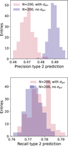 |
Fig. 7 Posterior distributions for the Type 2 precision (top) and recall predictions (bottom) from fitting the labeled dataset N = 200 times. The blue distribution indicate the value obtained from N RF reconstructions without inclusion of measurement errors, while the red distribution correspond to the reconstructions of the measurement uncertainty propagated pseudo-sets. In certain cases, the performance of the classifier is overestimated when photometric uncertainties are not taken into account. |
Precision and recall scores and uncertainties for Type 1 and Type 2 prediction using N = 200 fits to pseudo-sets with measurement uncertainties.
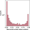 |
Fig. 8 Histogram of the averaged reconstructed obscuration values for all unlabeled data. While the majority of sources have an obscuration value equal to 0 or 1, a non-negligible number of them lie in the region between the two. |
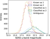 |
Fig. 9 SDSS u-band magnitude for all labeled and reconstructed datasets. The unlabeled sources classified as Type 2 AGN are fainter than the labeled Type 2 sources, which have made the photometric limit criteria for SDSS spectroscopic observations. In general, obscured AGN have a fainter optical spectra than unobscured ones. |
5 Machine learning for AGN property estimations
The following section presents the detail of selecting a suitable machine learning model to predict the parameters of Table 2, using the features presented in Table 1 as inputs. Since redshift measurements are available for almost half of the 21 050 AGN sources (but not for the other), we trained and tested two separate models, which we call MLW/Z, where z is added as an input and MLWo/z, where z is one of the outputs of the regressor. Just as is was done in Sect. 4 for ML classification, we develop how measurement errors are taken into account in ML regression using the pseudo-sets generated, thereby offering a more complete picture of the performance and quality of the reconstruction. For the training, we transformed our target parameters: z, LX, LBol MBH, and λEdd are often expressed in log scale to representatively describe the span of values across several decades.
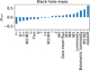 |
Fig. 10 Bar chart showing the Pearson correlation score of input variables and the black hole mass, from the training sample data. The redshift, luminosity, and bolometric luminosity correlations are included in this chart, since z (and thus LX) are known for almost half of the sources, and the outputs will be predicted before the black hole mass, underlining the logic behind the chain regression. |
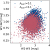 |
Fig. 11 W1–W2 magnitudes as a function of W2–W3 magnitudes for sources in the training sample with low (red dots) and high (blue dots) λEdd, The low and high samples are separated by the median value of the λEdd distribution, 0.1. |
5.1 Exploratory data analysis
Before choosing and training a machine-learning algorithm on the SPIDERS sample, we explored the relationship between the input variables and the target parameters. Figure 10 shows the sorted Pearson’s correlation coefficients for all inputs and one of the outputs, the black hole mass of the AGN. The relative IR and optical color magnitudes demonstrate the highest level correlation. This is even more visually evident when one looks, once more, at the IR color-color plot in Fig. 11. The scatter plot presents the W1/W2 versus W2/W3 A11WISE colors for AGNs with λEdd < 0.1 and λEdd > 0.1, the median value of λEdd in the training sample. We observe that strong accretion disks (higher λEdd) are redder in both W1/W2 and W2/W3 than lower λEdd values. These clear connections between IR photometry and spectroscopic observables, already accessible with a naive and straightforward data analysis, are encouraging indications that our goal – the estimation of AGN physical properties - is suited for a machine-learning task.
5.2 Machine learning model parameters
Ours is essentially a multi-dimensional linear regression task, with 18 multi-wavelength inputs, listed in Table 1, and 5 or 6 target parameters, depending on whether z is known for a source (see Table 2). Many ML applications are readily available to use for such a supervised learning task notably through the scikit-learn python library (Pedregosa et al. 2011). We used a single-output, multi-step chain regression (Demirel et al. 2019) so that the ML model can learn the correlations between target parameters, as previously done in Cunha & Humphrey (2022). In the first pass of the chain regressor, the initial 18 inputs are used to predict the first output, namely, the redshift z. In the next pass, the model takes 18+1 inputs, the extra-one being the predicted z, and outputs the next parameter, LX, and so on.
5.2.1 Selection of the ML model
We detail in this section our non-exhaustive search for the most suitable estimator. All supervised learning ML models essentially learn a mapping of inputs to outputs given an example of such a map. However, there is a plethora of model types available to choose from. For instance, linear models expect the output to be a linear combination of the features: certain regressors simplify the model by introducing penalty coefficients that will minimize (in the case of ridge regression Hilt et al. 1977) or reduce (for Lasso regression Tibshirani 1996) the input parameters, if some are found to contribute less to the learning. This procedure, called regularization, aims to reduce the overall error in the validation dataset. On the other hand, support vector regression (SVR), an application of the kernel-based support vector machines (Cortes & Vapnik 1995), allows us to tune the tolerance, e, to such errors, while introducing non-linearity parametrization through hyperplane fits to the data. Non-linearity is also a feature of neural networks, for instance, in a multi-layer perceptron (MLP; Murtagh 1991), via an activation function connecting the neural layers. Finally, decision tree predictors, such as random forests (Breiman 2001), also present the advantages of handling non-linear relationships between the input and output parameters. We compare these different ML models in the next section.
5.2.2 Model evaluation
To determine the best model, performance metrics are defined based on the validation dataset, where ytrue and yreco are known. We again used a K-fold cross validation method to insure a non-biased evaluation of the model, as each sample (in our case, each AGN source), will be used as a validation point once, and as a training set k – 1 times: the following metrics are thus calculated for a sample size Ν = 7616. As is common for regression problems, we use the R2 score, also called coefficient of determination, for each parameter to assess the performance of each model. This coefficient is calculated as:
 (6)
(6)
with the numerator being the residual sum of squares, and the denominator the total sum of squares. For a perfect regressor, we have R2 = 1. Figure 12 presents the target-by-target comparison between the two linear models (ridge and Lasso regression), a support vector regression model, a multi-layered perceptron (MLP) deep neural network model10, and a RF regressor. We stress that for this test, none of the model parameters have been tuned. The RF model is better at predicting all target outputs, in particular MBH, LEdd, and λEdd, with the SVR model coming in closely. This trend is also confirmed in the more difficult case of unknown z, represented by open circles in Fig. 12. From a pragmatic aspect, the runtime speed and low number of tuning parameters of the RF regressor were clear advantages compared to the vast phase space of MLP neural networks, for instance.
Once the performance of the RF model has been assessed, we completed a grid search over its hyperparameters to find their optimal values: the maximum depth, that is, the number of splits that each decision tree is allowed to make, the maximum number of features considered on a per-split level and the number of estimators, and the number of decisions trees in the forest. This step is important as the final result can quite vary between default and optimized parameters. We summarize the final parameters of the machine learning model that is selected for training in Table 4.
Properties of the final RF regressor ML-model properties chosen to be trained on.
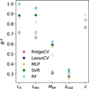 |
Fig. 12 Comparison of R2 for ML-models tested on all target parameters. Full circles represent MLw/z and open circles MLwo/z, the learning done for sources with unknown redshift. The RF algorithm performs best on crucial variables (MBH and λEdd). |
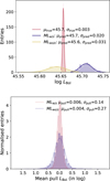 |
Fig. 13 Top: true (red), and predicted distributions reconstructed Ν times with MLw/z (purple) and MLwo/z (yellow) of the bolometric luminosity for a training source. The true value is represented by a normal distribution by taking into account the measurement error σtrue and assuming it to be gaussian. Bottom: mean pull distribution for the LBo] for all training sources, taking all μtrue – μpred values for MLw/z (red) and MLwo/z (purple). |
5.2.3 Regression metrics on Ν pseudo-sets
As was done for the classification task, we then used the Ν = 200 pseudo-sets to propagate both the uncertainties in the photometric measurements in the training and reconstructed datasets, as well as fluctuations of the regressor’s reconstruction. Here, we adopt an iterative method once more, where, for each i-th training sample, Ti, that the RF model is fitted with, values of Ti are predicted (for performance evaluation studies). This i-th fitted RF is then used to reconstruct the target parameters in Ci, which is the i-th pseudo-set of the unreconstructed catalog. The process was repeated Ν times.
The top panel of Fig. 13 displays the true and predicted distributions for the bolometric luminosity of a single source in the training sample. Here, μtrue and σtrue are given by the SPIDERS-AGN catalog for all target parameters and all sources, while μpred and σpred were obtained by fitting a Gaussian function to the Ν = 200 reconstructed values for each source. From these, we constructed the “pseudo-pull” distribution, μtrue – μpred. We note how, in this single source, the MLw/z (purple) and MLwo/z (yellow) recontructed values of LBol are multiple σpred apart. This is also clear from the bottom panel of Fig. 13, which shows the distribution of all pulls for the reconstructed LBol. Here, the difference in the quality of reconstruction between MLw/z and MLwo/z is apparent in the greater smearing of the pull distribution.
The precision of the reconstruction is also derived from the normalized median absolute deviation σNMAD = 1.48 × median (|Δμ – median(Δμ) | /μtrue, expressed in %, with Δμ = μtrue – μpred. It is a robust measure of the deviation, one that is insensitive to outliers.
Finally, the last metric we establish is the contamination level of the reconstruction: for each bin in μtrue, we look at the μpred distribution and fit a Gaussian probability density function (PDF), as seen in Fig. 14. We then defined the contamination to be the overlapping area between the lowest and highest true intervals reconstructed PDF, represented by the hashed area in Fig. 14. In the case of the λEdd parameter, it is the measure of how often our ML-model mistakes a low accretion-rate AGN with a high accretion-rate AGN and vice versa. This is a useful measurement in the event that the regressor lacks the precision to carry on single source studies, but still provides enough information to consider the features of a larger population, as it does for λEdd. Thus, even though the mean of the binned reconstructed values do not correspond to the center of the true bins, the scaling relation between lower and higher λEdd is preserved.
All performance metrics described in this section are presented in Table 5 for the MLw/z and MLwo/z cases. In the following section, we discuss in greater details the ability of our ML model to predict the physical parameters of AGN cores.
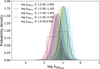 |
Fig. 14 Distributions of |


5.3 Prediction performance
Figures 15 and 16 summarizes the performance of the RF for the case with (MLw/z) and without redshift (MLwo/z), respectively. Each bin of the response matrix is normalized to the true bins (by column). The matrix elements represent the probability for an AGN with target parameter Ptrue to be reconstructed with a value Ppred. The error on the reconstructed value σpred for each source is used to weight to the histogram.
5.3.1 Prediction of z
Determining redshifts through spectroscopic or photometric means has always been a primary goal of large AGN surveys. The overall performance of the ML-model in predicting the redshift up to z ~ 2.5 can be seen on the top left matrix of Fig. 16. To better evaluate the accuracy of | Δz | /(1 + ztrue) (Δz = zpred –ztrue), we modified our formula of σNMAD slightly to match the same estimator found in the literature (Brammer et al. 2008; Luo et al. 2010), such that σNMAD=1.48× median(|Δz-median (Δz) |/(l + ztrue). An outlier is defined as having | Δz /(l + ztrue) > 0.15 (see Fig. 17). For redshifts reconstructed with the best parameter RF, we find the rate of outlier to be 1.17% and σNMAD=0.041 (accuracy of 4.1%), performing just as well as the estimation of photometric redshifts using template-fitting methods (Pforr et al. 2019; Salvato et al. 2011; Luo et al. 2010; Ilbert et al. 2006; Bolzonella et al. 2000; Baum 1962).
The regressor’s reconstruction slightly worsens as we move into higher z: this is simply because the SPIDERS dataset provides few sample for the supervised learning to train on, as the distribution of z decreases sharply (see Fig. 19). The ML reconstruction of redshifts proves to be a very reliable estimator for a crucial parameter for AGN studies, and one that could be adapted to different depths given an appropriate training dataset.
5.3.2 LX and LBol
Naturally, once the model has an estimation for z, it can easily find the appropriate regression for LX, given that the X-ray flux is one of the model’s inputs. As anticipated, the X-ray luminosity is predicted with high accuracy and precision: when z is known, the error on the estimate is log(LX/erg s−1) ~ 0.037 and rises to ~0.193 when z is reconstructed. The bolometric luminosity LBol, being the convolution of multiple wavelength observations presents the first moderate challenge for the model to predict: however, it gives reliable reconstructed values, with σerr. = 0.142 (0.268) for MLw/z (MLwo/z). In general, the performance worsens slightly as we move into the tails of the bin edges and the data in sample we have trained on become scarce: the reconstructed parameters tend to be overestimated for low values of the true parameter, while they are underestimated for high values.
5.3.3 Prediction of MBH and λEdd
When it comes to estimations of MBH, the R2 score is 0.62 for MLw/z and 0.48 for MLwo/z, and the width of the pull σpull goes from 0.56 to 0.65 in units of log(M⊙). This uncertainty in the truth reconstruction is slightly higher than the systematic uncertainties in MBH from velocity dispersion measurements (Tremaine et al. 2002; Hu 2008; Koss et al. 2022; Ricci et al. 2022).
The Eddington ratio to be the hardest parameter to predict, since the errors from the previous predictions get propagated and compounded. However, the RF regressor manages to reconstruct it with a satisfying accuracy: the R2 score is 0.35 for both MLw/z for MLwo/z, and the width of the pull σpull is about 0.54 in units of log(λEdd). It is also the characteristic for which the prior knowledge of z has the least impact, although the reconstruction of both LBol and MBH is markedly better in the MLw/z. To understand why that is, we can study the correlations between the predicted parameters in the form of the mean pull values μpull. Figure 18 presents the correlations of pulls between all parameters, for MLw/z (red) and MLwo/z (blue). In the case where the redshift, z, is the first predicted parameter in the chain regression (MLwo/z), all subsequent parameters remain more or less strongly correlated to one another, as the Pearson’s correlation score can attest to. Specifically, if a prior parameter is poorly reconstructed, the subsequent one will be as well. On the other hand, no such correlations between the pulls is found in the case of MLw/z, where LX is the first estimated parameter.
Results of the best-tuned RF estimators, MLw/z and MLwo/z, for the performance metrics presented in Sect. 5.2.2 for all target parameters.
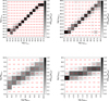 |
Fig. 15 Normalized performance matrices for ML-estimator with known redshift as an input (MLw/z). The true and reconstructed parameters are plotted on the x and y axis, respectively. The error on the reconstruction is used as a weight to the histogram. |
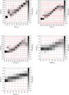 |
Fig. 16 Normalized performance matrices for the ML-estimator without a known redshift as an input (MLwo/z). The matrix for the reconstructed z is added to the variables already presented in Fig. 15. |
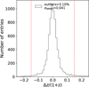 |
Fig. 17 Distribution of the predicted redshift, zpred, accuracy derived with the true spectroscopically measured redshift, ztrue. The dashed red lines represent the limit beyond which a prediction is counted as an outlier. |
6 Reconstruction of the full catalog
In the following section, we take a closer look at the estimated AGN physical parameters for the ~22 000 sources without spec-troscopic information. As was done for the training sample, all AGN were reconstructed N = 200 times with the method outlined in Sect. 3. The mean μreco and standard deviation σreco from a Gaussian fit to the posterior probability distribution are recorded for each source11. Pointers are encoded in σreco to the regressor’s ability to reconstruct AGNs that are further away from the input range, revealing differences between population type. The distribution of z for the 9944 sources in the full catalog is overlaid on top of that of the training sample in Fig. 19: the median is  and we can observe that the range of z follows a similar trend, with slightly more AGN sources in z > 1 range.
6.1 Reconstruction quality for type 1 and type 2 AGN
Although the ML model was trained on a sample of type 1 AGNs only, we reconstructed the 3062 sources in our catalog identified as type 2 AGNs, using the classifier and criteria presented in Sect. 4. Figure 20 presents the distributions of the reconstruction uncertainty σreco on the MBH parameter for type 1 and 2 AGNs, with and without known z. Sources reconstructed with MLw/z have smaller uncertainties, following the results from the training sample (see Sect. 5), and the RF has a harder time estimating parameters for type 2 AGNs. The shape of the distribution informs that the regressor is able to reconstruct the MBH type 2 AGNs with both known and unknown z (purple and green distributions).
Considering what was already shown in Fig. 9, we know that many AGNs classified as type 2 fall into the faint end of the optical magnitude distribution (e.g., SDSS u-band mag >22) (Antonucci 1993; Hickox & Alexander 2018). The fainter the source, the more outside of the bounds of u magnitude the ML model has trained on, the greater the uncertainty on the reconstructed parameter. This is yet another piece of information gained by propagating the input uncertainties and reconstructing each source iteratively. In particular, the difficulty the regressor encounters when estimating points outside of its known range is translated in the spread of the posterior distribution for all output parameters.
6.2 Removal of outliers
As a last step, we removed the sources in the final sample for which the reconstructed values lie beyond the phase space of the training sample target parameters. This requirement for z removes 297 sources alone.
In addition, we cross-matched our sources with the Fermi 4FGL catalog (Ajello et al. 2020), to eliminate any AGNs already identified as a blazar. Requiring a wide matching radius of 10 arcsec, 24 sources were removed, bringing the final number of outliers to 319. In total, 21 050 AGNs with newly reconstructed physical parameters are added to the catalog, on top of the 7613 remaining SPIDERS AGN sources.
6.3 Type 1 AGN studies
We now focus on the AGNs classified as type 1, as that population follows the training dataset more closely. Figure 21 presents the bolometric luminosity versus BH mass (top panel) for the type 1 AGNs presented in this work and the SPIDERS AGNs: the reconstructed sample is well bounded by the Eddington limit. The bottom panel of Fig. 21 shows the Eddington ratio as a function of the redshift for the same subsamples. As the response matrices in Figs. 15 and 16 have shown, the ML model is not very apt with respect to reconstructing the extreme cases in the lower and upper tails of the target parameter distribution. That is to say, it will overestimate low values and underestimate higher ones: this is indeed visible in the bottom panel of Fig. 21, where the reconstructed samples occupy a smaller region of the log λEdd space than the SPIDERS AGN do.
The top panel of Fig. 22 presents the AGN number source density over a wide range of redshifts for several bins in bolo-metric luminosity. Reconstructed type 1 AGNs are shown in full circles and SPIDERS AGNs are represented in open circles for the same luminosity bins. The same trends are observed in the spectroscopically observed and reconstructed samples: the number density of lower-luminosity AGN peaks later in cosmic time than that of more luminous ones: this effect is known as AGN downsizing (Ueda et al. 2003, 2014; Miyaji et al. 2015; Brandt & Alexander 2015). The bottom panel of Fig. 22 shows the black hole masses of these sources, using the same binning in LBol. Although the tails of the distributions are not well represented in the reconstructed sample when matched to their SPIDERS AGN counterparts, it is important to note that not only does the scaling trend of increasing MBH with LBol remain, but the peaks of the distribution are also coincident between the spectroscopically observed and ML reconstructed type 1 AGN samples. Although deriving a luminosity function from these AGNs would require the non-trivial correction of the number density for detection and selection efficiencies and biases (Schulze et al. 2015; Weigel et al. 2017; Ananna et al. 2022), the two panels of Fig. 22 show the accurate description of AGN behavior in a multidimensional phase space (z, LBol, and MBH) when compared with the spectroscopically measured SPIDERS AGN sample.
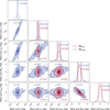 |
Fig. 18 Correlation between pull values for all parameters for MLw/z (red) and MLwo/z (blue). The quality of reconstruction, represented by the mean pull value, is more correlated between the variables in MLwo/z than it is for MLw/z. The vertical dashed lines in the histograms indicate the 0.16 and 0.84 quantites of the distributions, and the numbers show the respective medians and 0.16 and 0.84 quantites. |
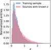 |
Fig. 19 Distribution of z for the training sample coming from the SPIDERS AGN catalogue (blue) and the subsample of AGN sources in the reconstruction sample for which z is known (red). |
6.4 Validation with BASS DR2 catalog
The BAT AGN spectroscopic survey (BASS) is a hard X-ray spectroscopic survey with the Swift instrument that characterizes the physical parameters (z, Lbol, MBH and λEdd) of ~1000 AGNs selected in the hard (14–195 keV) X-ray (Koss et al. 2022). The second data release (DR2) offers itself as an ideal independent validation set for our ML study. We cross-matched our catalog with the BASS DR2, demanding a strict 1 arcsec maximum radius, and found 196 counterparts; of these, 64 come from the SPIDERS AGN training sample (Coffey et al. 2019) and 115 were ML-reconstructed. We compared the key AGN parameters from this work and the BASS catalog in Fig. 23. The red points represent the SPIDERS-AGN values, allowing for a direct comparison from two optical spectroscopy measurements, while the blue points represent ML-reconstructed values. We observe that for z, the three datasets are in excellent agreement, while 67% (65%) of ML-reconstructed (SPIDERS-AGN) LBol are within 0.5 dex of their BASS counterpart measurement.
For black hole masses, while the correlation scores are lower overall, the reconstructed values are well validated by the BASS survey values: 64% (77%) of ML-reconstructed (SPIDERS-AGN) MBH values are within 0.5 dex of their BASS counterpart.
The Eddington ratio, however, shows the greatest level of discrepancy, with a visible systematic shift between spectroscopic measurement. While they are closer to one another than ML-reconstructed λEdd values, the differences might be explained by the two instrument’s observations of changing-look AGN during different phases of accretion activity, with the emergence or disappearance of broad emission lines (Ulrich et al. 1997; Soldi et al. 2014; Mereghetti et al. 2021; Ricci & Trakhtenbrot 2023).
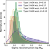 |
Fig. 20 Uncertainty σreco on the log of the reconstructed black hole mass MBH for Type 1 and 2 AGN, with and without z information (estimated with MLw/z and MLwo/z respectively). The & values correspond to the median of their distributions. All AGN types can be reconstructed, as proven by their characteristic PDF structures, although the overall reconstructed uncertainties worsen as a function of the AGN class. |
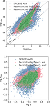 |
Fig. 21 Top: scatter plot of LBol as a function of MBH for the SPIDERS AGN (blue dots), and reconstructed AGN classified as Type 1. AGN with known z measurement are shown in red dots, and those with reconstructed z are represented in green. Bottom: Same three samples for the λEdd vs. z distribution. |
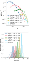 |
Fig. 22 Top: AGN downsizing: comoving number density vs. red-shift for Type 1 AGN from this work’s catalogue (full circles) and the SPIDERS AGN catalogue (open circles) for different bins of LBol in units of log(erg s−1). Bottom: distribution of MBH for the same bins of bolometric luminosities, for the reconstructed AGN (colored bars) and SPIDERS AGN (colored steps). A flat ΛCDM cosmology with H0 = 70 km s−1 Mpc−1 ΩΜ = 0.3, and ΩΛ = 0.7 is assumed to calculate the comoving number density. |
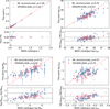 |
Fig. 23 Comparison of AGN physical paramaters from the BASS, SPIDERS-AGN and ML-reconstructed catalogues for 196 cross-matched sources: the redshift z (top left), LBol (top right), MBH (bottom left) and λEdd (bottom right). The bottom panel of each subfigure represents the difference of the BASS survey’s and this work’s values. The horizontal grey dashed line show the ± 0.5 dex level. |
7 Summary and conclusions
We have released the first photometry based estimates of bolometric luminosity LBol, black hole mass, MBH, and Eddington ratio, λEdd, for 21 050 sources ranging over 6 dex in luminosity and up to z=2.4 in redshift. For 11 363 of these sources, the redshift was previously determined spectroscopically and was used in the estimation of the remaining parameters, as well as for the verification of the redshift estimate. For 11 363 sources without a previously known redshift, the reconstructed z is provided, with excellent accuracy. An uncertainty is given for all estimated parameters, thanks to a simulation based technique which incorporates measurement errors in the fit and reconstruction of the ML regressor. In addition, we have demonstrated how ML classification tools can help identify obscured AGN, a crucial challenge in the field (see review by Hickox & Alexander 2018). Finally, we used the existing BASS survey catalog (Koss et al. 2022) to benchmark this work’s ML-reconstructed values with an independent spectroscopic measurement of AGN physical parameters.
While the addition of ~21 000 AGN sources from this catalog might not dramatically improve our knowledge of the luminosity function, considering that the 8000 SPIDERS AGN sources were measured with greater accuracy in the same phase space, the release of this new dataset is of particular use for multimessenger astronomy studies, where one needs to know these physical parameters for a large sample of sources, while maximizing the sky coverage. AGN have been favored to be strong cosmic ray emitters (Halzen & Zas 1997; Murase 2022; Murase & Stecker 2023), with the recent discovery showing the nearby obscured AGN NGC 1068 to be a steady source of neutrinos (IceCube Collaboration 2022). Searches for a cumulative signal from different AGN populations, such as Abbasi et al. (2022), can help characterize which sources contribute most to the flux of neutrinos, based on their accretion parameters. By strategically targeting a subset of sources observed spectroscopically, we would be able to train similar ML-algorithms and reconstruct a larger sample of photometrically measured AGNs. The method can easily be expanded to other cosmic demographics (e.g., higher z) granted a corresponding dataset is provided to train a ML algorithm. In this work, we were limited by demanding that sources had been observed with SDSS photometry: this constrained the coverage to a quarter of the full sky. A natural next step would be to expand the optical sky coverage by cross-matching sources with the Pan-STARRS 3π survey Flewelling et al. (2020), and recover most AGNs identified with IR and X-ray telescopes. Finally, eROSITA has been scanning the full-sky with unprecedented sensitivity in the soft (0.2–2.3 keV) and hard (2.3–8 keV) bands (Merloni et al. 2012; Predehl et al. 2021), having recently published its first data release (Merloni et al. 2024). Incorporating this dataset will also offer new understanding of obscured AGNs, as harder X-ray photons are transparent to obscuring dust (Salvato et al. 2022; Waddell et al. 2024a,b).
Acknowledgements
The author wishes to thank Iftach Sadeh, Anna Franckowiak, Sjoert Van Velzen, Jannis Necker, Simone Garrapa and Jonas Sinapius for their fruitful comments and support. Timo Karg is to be thanked for helping with various technicalities.
Appendix A Catalog column description
The result of the work presented in this paper has been compiled into a single catalog available online12. This includes the 21 050 reconstructed sources, with results from the obscuration classifier and estimation of z, LX, LBol, MBH, LEdd, and λEdd with associated reconstruction uncertainties.
In addition, the 7613 SPIDERS sources used in the training sample are also included. A description of the catalog’s columns is given below. Features providing X-ray, IR, and optical information were taken from the references listed in Table 1.
Column 1— X-ray detection: Flag indicating whether the X-ray source was detected in the 2RXS or XMMSL2 survey (Boller et al. 2016; Saxton et al. 2008).
Column 2— Name: X-ray identifier from 2RXS or XMMSL2 survey.
Column 3-4— RA, DEC: Right ascension and declination of the X-ray detection (J2000) in degrees.
Column 5-6— Flux, flux error: X-ray flux and error converted to the 0.5-2 keV band in log10(erg cm−2s−1).
Column 7— ALLWJD: WISE All-Sky Release catalog name (Cutri et al. 2021)
Column 8-9— ALLW_RA, ALLW_DEC: J2000 A11WISE right ascension and declination, in degrees.
Column 10-13—— W[1234]: A11WISE Vega magnitude in the Wl, W2, W3, and W4 bands.
Column 14-17—— W[1234] error: A11WISE Vega magnitude errors in the Wl, W2, W3, and W4 bands.
Column 18-19— Gaia mean flux, Gaia mean flux error: Gaia mean flux and error in units of e-s−1.
Column 20— CLASS: Broad spectral classification computed by the SDSS-DR16 spectroscopic pipeline.
Column 21— SUBCLASS: Detailed spectral classification computed by the SDSS-DR16 spectroscopic pipeline.
Column 22-26— psfMag_[ugriz]: Point spread function magnitude of the optical counterpart to the IR source in the ugriz band (mag, AB).
Column 27-31— psfMagErr_[ugriz]: Uncertainties on the PSF magnitude in the ugriz band (mag, AB).
Column 32— z: Redshift of the source, and uncertainty (in log10).
Column 33— z error: Uncertainty on the redshift.
Column 34— Luminosity: X-ray luminosity in the 0.5-2 keV band in log10(erg.s−1).
Column 35— Luminosity error: Uncertainty on the X-ray luminosity in the 0.5-2 keV band in log10(erg.s−1).
Column 36— Bolometric luminosity: Bolometric luminosity in log10(erg.s−1).
Column 37— Bolometric luminosity error: Uncertainty on the bolometric luminosity in log10(erg.s−1).
Column 38— Black hole mass: BH mass in log10(M⊙).
Column 39— Black hole mass error: Uncertainty on the BH mass in log10(M⊙).
Column 40— Eddington luminosity: Eddington luminosity in log10(erg.s−1).
Column 41— Eddington luminosity error: Uncertainty on the Eddington luminosity in log10(erg.s−1).
Column 42— Eddington ratio: Eddington ratio in log.
Column 43— Eddington ratio error: Uncertainty on the Eddington ratio in log.
Column 44— Reconstructed: Flag indicating whether the source and values from columns 32-43 come from this work’s ML reconstruction (ffag==l) or from the SPIDERS AGN spectroscopic catalog (flag==0) (Coffey et al. 2019).
Column 45— Known z: Flag indicating whether the red-shift values from column 32-33 come from this work’s ML reconstruction (flag==0) or from the previous spectroscopic visual derived redshift (flag==l) (Dwelly et al. 2017; Véron-Cetty & Véron 2010).
Column 46— Obscuration: Value between 0 and 1 indicating whether the source is obscured (obscuration ~ 1) or not (obscuration ~ 0), from the ML classifier presented in Sect. 4.
Column 47— Obscuration error: Uncertainty on the obscuration value.
Appendix B Feature selection of type 2 AGNs
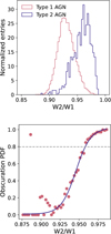 |
Fig. B.1 Obscuration PDF definition. (Top) distribution of the SDSS sources classified as Type 1 and Type 2 AGN as a function of W2/W1 magnitudes. (Bottom) Obscuration PDF derived from the left figure and Eq. B.1 from a sigmoid fit to the points. The dashed gray line represents the cut threshold which defines whether an AGN is of Type 1 or 2. It was chosen by doing a grid search over Obscuration PDF values and choosing the value giving the best F1-score. |
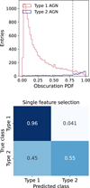 |
Fig. B.2 Obscuration PDF precision recall curve definition. (Top) Distribution of SDSS defined Type 1 and 2 AGN as a function of their derived Obscuration PDF. The vertical gray dashed line represents the threshold value giving the optimal classification perfomance. (Bottom) Confusion matrix derived from the left distribution, by scanning through values between 0 and 1 and calculating the precision and recall. |
Using the known SDSS classification for the subsample of 9535 AGN, we can distinguish type 2 from type 1 galaxies in the W2-W1 space (see top panel of Fig. B.1, following the method outlined in Abbasi et al. (2022). We can use these two distributions to define an “obscuration” PDF as:
 (B.1)
(B.1)
where Ƥ(typel) and Ƥ(type2) are the probabilities of an AGN being of type 1 or of type 2, respectively, according to the normalized histograms of Fig. B.1
By applying Equation B.1 to these two distributions, we obtain the obscuration PDF shown in the bottom panel of Fig. B.1, with the blue line representing a sigmoid fit to the data points. Using this fitted function, we obtain the distribution of SDSS-classifled type 1 and type 2 AGN as a function of the derived obscuration PDF (top panel of Fig. B.2. By scanning through obscuration PDF values between 0 and 1, we can calculate the precision and recall for each threshold , based on the definitions given in Sect. 4. This then gives us confusion matrix presented in the bottom panel of Fig. B.2. Using this single feature classification, we reach a type 1 TNR of 96%, but a poor type 2 identification power with the TPR at 55% only, for an optimized obscuration PDF threshold of 0.80.
Appendix C Handling of null entries
The supervised ML algorithm cannot accept null entries for any of the features. This is true for the training sample, as well as the catalog that is to be reconstructed. As explained in Sect. 2.4, demanding SDSS photometry observations for all AGN sources represents the greatest cut that can be applied to the data, however, some features still remain incomplete. Instead of indiscriminately removing these data points, we looked for correlations between fully complete features and partially incomplete ones: we fit the function which describes the relationship in that parameter space in order to derive dummy values. In the SPIDERS catalog, 685 (278) sources have A11WISE W3 (W4) magnitudes but are missing corresponding photometric error measurements. Similarly 278 SPIDERS have no entries for the Gaia mean flux and errors. In total, the training sample has 918 sources with null entries, while this number is 9337 for the reconstructed catalog. The top panel of Fig. C.1 shows the W4 magnitude as a function of the W4 error for AGNs with complete information in the SPIDERS sample. An exponential function is fit and W4 error are interpolated for sources which are missing entries (yellow points). The soft X-ray flux F0.5–2kev is also used to derive a value for the Gaia mean flux using a log-log fit. The relationship between the Gaia mean flux and its associated error itself is then used to complete the error column.
We studied the effect of creating synthetic points for IR errors and Gaia mean fluxes and errors, in the simulation-based approach (see Sect. 3) chosen. Fig. C.2 shows pull distributions for MBH and λEdd as a function of whether the AGN sources have any synthesized entries, for both MLw/z and MLw/oz. Comparing the standard deviation σ from the Gaussian, we note a degradation of ~ 10% in the fit resolution when synthesized points are added. However, points with missing entries are those which lie on the fainter end of the phase space (see right panel of Fig. C.2), in the tail of the training sample’s distribution: these points are intrinsically harder to reconstruct with the smaller sample used to train to the ML regressor. Similarly, when looking at the uncertainties for the ML-reconstructed (unknown) catalog, AGN sources with synthetic entries have a larger σerr, as is shown for MBH reconstruction on the left panel of Fig. C.3. However, again, as the right panel of the figure indicates, the ratio of type 2 sources within the synthetic sample is far greater, so much so that the error PDF plot is equivalent to the one shown in Fig. 20; namely the synthetic points have a slightly poorer reconstruction because they are faint.
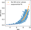 |
Fig. C.1 Handling of null entries: W4 error values for points missing one are estimated (yellow points) using an exponential fit to the W4 error vs W4 plane. |
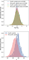 |
Fig. C.2 Pull distribution with gaussian fits for MBH (top) help us study the effect of creating synthetic entries in the training sample. On average, the reconstruction resolution degrades by -10% when synthetic points for IR errors and/or Gaia mean fluxes are included. AGN sources with synthetic entries lie on the fainter end of the multi-wavelength spectra (SDSS u-mag shown on the bottom panel). |
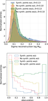 |
Fig. C.3 Effect of synthetic entries generation for the reconstructed sample. Top: error distribution for the reconstructed MBH. Bottom: reconstruction obscuration level as a function of several subsamples. AGN sources with synthetic entries for IR errors and/or Gaia mean fluxes are the same dim sources that make up the Type 2 AGN sample from Fig.20. |
References
- Aartsen, M. G., Abraham, K., Ackermann, M., et al. 2017, ApJ, 835, 45 [Google Scholar]
- Aartsen, M. G., Ackermann, M., Adams, J., et al. 2020, ApJ, 898, 117 [NASA ADS] [CrossRef] [Google Scholar]
- Abbasi, R., Ackermann, M., Adams, J., et al. 2022, Phys. Rev. D, 106, 022005 [Google Scholar]
- Abbasi, R., Ackermann, M., Adams, J., et al. 2023, ApJ, 949, L12 [NASA ADS] [CrossRef] [Google Scholar]
- Achterberg, A., Ackermann, M., Adams, J., et al. 2006, Astropart. Phys., 26, 282 [NASA ADS] [CrossRef] [Google Scholar]
- Ahumada, R., Allende Prieto, C., Almeida, A., et al. 2020, ApJS, 249, 3 [NASA ADS] [CrossRef] [Google Scholar]
- Ajello, M., Angioni, R., Axelsson, M., et al. 2020, ApJ, 892, 105 [NASA ADS] [CrossRef] [Google Scholar]
- Alam, S., Albareti, F. D., Prieto, C. A., et al. 2015, ApJS, 219, 12 [NASA ADS] [CrossRef] [Google Scholar]
- Ananna, T. T., Weigel, A. K., Trakhtenbrot, B., et al. 2022, ApJS, 261, 9 [NASA ADS] [CrossRef] [Google Scholar]
- Antonucci, R. 1993, ArA&A, 31, 473 [NASA ADS] [CrossRef] [Google Scholar]
- Arenou, F., Luri, X., Babusiaux, C., et al. 2017, A&A, 599, A50 [NASA ADS] [CrossRef] [EDP Sciences] [Google Scholar]
- Assef, R. J., Stern, D., Kochanek, C. S., et al. 2013, ApJ, 772, 26 [Google Scholar]
- Barandela, R., Sánchez, J. S., García, V., & Rangel, E. 2003, Pattern Recognit., 36, 849 [NASA ADS] [CrossRef] [Google Scholar]
- Batista, G. E. A. P. A., Prati, R. C., & Monard, M. C. 2004, ACM SIGKDD Explor. Newslett., 6, 20 [CrossRef] [Google Scholar]
- Baum, W. A. 1962, Problems of Extra-Galactic Research, 15, 390 [NASA ADS] [Google Scholar]
- Blanton, M. R., Bershady, M. A., Abolfathi, B., et al. 2017, AJ, 154, 28 [Google Scholar]
- Boller, T., Freyberg, M. J., Trümper, J., et al. 2016, A&A, 588, A103 [NASA ADS] [CrossRef] [EDP Sciences] [Google Scholar]
- Bolton, A. S., Schlegel, D. J., Aubourg, et al. 2012, AJ, 144, 144 [NASA ADS] [CrossRef] [Google Scholar]
- Bolzonella, M., Miralles, J. M., & Pelló, R. 2000, A&A, 363, 476 [NASA ADS] [Google Scholar]
- Bonjean, V., Aghanim, N., Salomé, P., et al. 2019, A&A, 622, A137 [NASA ADS] [CrossRef] [EDP Sciences] [Google Scholar]
- Brammer, G. B., van Dokkum, P. G., & Coppi, P. 2008, ApJ, 686, 1503 [Google Scholar]
- Brandt, W. N., & Alexander, D. M. 2015, A&ARv, 23, 1 [Google Scholar]
- Brandt, W., & Hasinger, G. 2005, ArA&A, 43, 827 [NASA ADS] [CrossRef] [Google Scholar]
- Breiman, L. 2001, Mach. Learn., 45, 5 [Google Scholar]
- Burbidge, G. R. 1958, PASP, 70, 83 [CrossRef] [Google Scholar]
- Chawla, N. V., Bowyer, K. W., Hall, L. O., & Kegelmeyer, W. P. 2002, J. Artif. Intell. Res., 16, 321 [CrossRef] [Google Scholar]
- Clarke, A. O., Scaife, A. M. M., Greenhalgh, R., & Griguta, V. 2020, A&A, 639, A84 [NASA ADS] [CrossRef] [EDP Sciences] [Google Scholar]
- Clerc, N., Merloni, A., Zhang, Y.-Y., et al. 2016, MNRAS, 463, 4490 [Google Scholar]
- Coffey, D., Salvato, M., Merloni, A., et al. 2019, A&A, 625, A123 [NASA ADS] [CrossRef] [EDP Sciences] [Google Scholar]
- Comparat, J., Merloni, A., Dwelly, T., et al. 2020, A&A, 636, A97 [NASA ADS] [CrossRef] [EDP Sciences] [Google Scholar]
- Cortes, C., & Vapnik, V. 1995, Mach. Learn., 20, 273 [Google Scholar]
- Cunha, P. A. C., & Humphrey, A. 2022, A&A, 666, A87 [NASA ADS] [CrossRef] [EDP Sciences] [Google Scholar]
- Cutri, R. M., Wright, E. L., Conrow, T., et al. 2021, VizieR Online Data Catalog: II/328 [Google Scholar]
- Dainotti, M. G., Bogdan, M., Narendra, A., et al. 2021, ApJ, 920, 118 [NASA ADS] [CrossRef] [Google Scholar]
- Demirel, K., Sahin, A., & Albey, E. 2019, in Proceedings of the 8th International Conference on Data Science, Technology and Applications (Prague, Czech Republic: SCITEPRESS – Science and Technology Publications), 267 [CrossRef] [Google Scholar]
- Dwelly, T., Salvato, M., Merloni, A., et al. 2017, MNRAS, 469, 1065 [Google Scholar]
- Edelson, R. A., Alexander, T., Crenshaw, D. M., et al. 1996, ApJ, 470, 364 [NASA ADS] [CrossRef] [Google Scholar]
- Elitzur, M., & Shlosman, I. 2006, ApJ, 648, L101 [Google Scholar]
- Elvis, M., Wilkes, B. J., McDowell, J. C., et al. 1994, ApJS, 95, 1 [Google Scholar]
- Feigelson, E. D., de Souza, R. S., Ishida, E. E., & Babu, G. J. 2021, Annu. Rev. Stat. Applic., 8, 493 [NASA ADS] [CrossRef] [Google Scholar]
- Ferrarese, L., & Merritt, D. 2000, ApJ, 539, L9 [Google Scholar]
- Flewelling, H. A., Magnier, E. A., Chambers, K. C., et al. 2020, ApJS, 251, 7 [NASA ADS] [CrossRef] [Google Scholar]
- Fotopoulou, S., & Paltani, S. 2018, A&A, 619, A14 [NASA ADS] [CrossRef] [EDP Sciences] [Google Scholar]
- Gaia Collaboration (Brown, A. G. A., et al.) 2018, A&A, 616, A1 [NASA ADS] [CrossRef] [EDP Sciences] [Google Scholar]
- Gebhardt, K., Bender, R., Bower, G., et al. 2000, ApJ, 539, L13 [Google Scholar]
- Ginsburg, A., Sipicz, B. M., Brasseur, C. E., et al. 2019, AJ, 157, 98 [NASA ADS] [CrossRef] [Google Scholar]
- Halzen, F., & Zas, E. 1997, ApJ, 488, 669 [NASA ADS] [CrossRef] [Google Scholar]
- Hasinger, G. 2008, A&A, 490, 905 [NASA ADS] [CrossRef] [EDP Sciences] [Google Scholar]
- Hickox, R. C., & Alexander, D. M. 2018, ArA&A, 56, 625 [NASA ADS] [CrossRef] [Google Scholar]
- Hilt, D. E., Hilt, D. E., Seegrist, D. W., States, U., & Northeastern Forest Experiment Station (Radnor, P. 1977, Ridge, A Computer Program for Calculating Ridge Regression Estimates (Upper Darby, PA: Dept. of Agriculture, Forest Service, Northeastern Forest Experiment Station) [Google Scholar]
- Hu, J. 2008, MNRAS, 386, 2242 [CrossRef] [Google Scholar]
- IceCube Collaboration (Abbasi, R., et al.) 2022, Science, 378, 538 [CrossRef] [PubMed] [Google Scholar]
- Ilbert, O., Arnouts, S., McCracken, H. J., et al. 2006, A&A, 457, 841 [NASA ADS] [CrossRef] [EDP Sciences] [Google Scholar]
- Khramtsov, V., Akhmetov, V., & Fedorov, P. 2020, A&A, 644, A69 [EDP Sciences] [Google Scholar]
- Kim, M., & Hwang, K.-B. 2022, PLoS ONE, 17, e0271260 [Google Scholar]
- Kochanek, C. S., Eisenstein, D. J., Cool, R. J., et al. 2012, ApJS, 200, 8 [Google Scholar]
- Kormendy, J., & Ho, L. C. 2013, ArA&A, 51, 511 [NASA ADS] [CrossRef] [Google Scholar]
- Koss, M. J., Trakhtenbrot, B., Ricci, C., et al. 2022, ApJS, 261, 1 [NASA ADS] [CrossRef] [Google Scholar]
- Laor, A. 2003, ApJ, 590, 86 [NASA ADS] [CrossRef] [Google Scholar]
- Li, C., Zhang, Y., Cui, C., et al. 2021, MNRAS, 506, 1651 [NASA ADS] [CrossRef] [Google Scholar]
- Luo, B., Brandt, W. N., Xue, Y. Q., et al. 2010, ApJS, 187, 560 [NASA ADS] [CrossRef] [Google Scholar]
- Lyke, B. W., Higley, A. N., McLane, J. N., et al. 2020, ApJS, 250, 8 [NASA ADS] [CrossRef] [Google Scholar]
- Lynden-Bell, D. 1969, Nature, 223, 690 [NASA ADS] [CrossRef] [Google Scholar]
- Magorrian, J., Tremaine, S., Richstone, D., et al. 1998, AJ, 115, 2285 [Google Scholar]
- Mainzer, A., Bauer, J., Grav, T., et al. 2011, ApJ, 731, 53 [Google Scholar]
- Mannheim, K. 1995, Astropart. Phys., 3, 295 [NASA ADS] [CrossRef] [Google Scholar]
- Matthews, T. A., & Sandage, A. R. 1963, ApJ, 138, 30 [CrossRef] [Google Scholar]
- Menzel, M.-L., Merloni, A., Georgakakis, A., et al. 2016, MNRAS, 457, 110 [Google Scholar]
- Mereghetti, S., Balman, S., Caballero-Garcia, M., et al. 2021, Exp. Astron., 52, 309 [NASA ADS] [CrossRef] [Google Scholar]
- Merloni, A., Predehl, P., Becker, W., et al. 2012, arXiv e-prints [arXiv:1209.3114] [Google Scholar]
- Merloni, A., Lamer, G., Liu, T., et al. 2024, A&A, 682, A34 [NASA ADS] [CrossRef] [EDP Sciences] [Google Scholar]
- Minkowski, R. 1960, ApJ, 132, 908 [NASA ADS] [CrossRef] [Google Scholar]
- Miyaji, T., Hasinger, G., Salvato, M., et al. 2015, ApJ, 804, 104 [Google Scholar]
- Murase, K. 2022, Science, 378, 474 [NASA ADS] [CrossRef] [Google Scholar]
- Murase, K., & Stecker, F. W. 2023, in The Encyclopedia of Cosmology, World Scientific Series in Astrophysics, 483 [Google Scholar]
- Murtagh, F. 1991, Neurocomputing, 2, 183 [CrossRef] [Google Scholar]
- Padovani, P., Alexander, D. M., Assef, R. J., et al. 2017, A&ARv, 25, 2 [Google Scholar]
- Pedregosa, F., Varoquaux, G., Gramfort, A., et al. 2011, J. Mach Learn. Res., 12, 2825 [Google Scholar]
- Pforr, J., Vaccari, M., Lacy, M., et al. 2019, MNRAS, 483, 3168 [Google Scholar]
- Plotkin, R. M., Anderson, S. F., Hall, P. B., et al. 2008, AJ, 135, 2453 [NASA ADS] [CrossRef] [Google Scholar]
- Predehl, P., Andritschke, R., Arefiev, V., et al. 2021, A&A, 647, A1 [EDP Sciences] [Google Scholar]
- Rees, M. J. 1984, ArA&A, 22, 471 [NASA ADS] [CrossRef] [Google Scholar]
- Rhea, C., Rousseau-Nepton, L., Prunet, S., et al. 2021, ApJ, 910, 129 [NASA ADS] [CrossRef] [Google Scholar]
- Ricci, C., & Trakhtenbrot, B. 2023, Nat. Astron., 7, 1282 [Google Scholar]
- Ricci, C., Walter, R., Courvoisier, T. J. L., & Paltani, S. 2011, A&A, 532, A102 [NASA ADS] [CrossRef] [EDP Sciences] [Google Scholar]
- Ricci, F., Treister, E., Bauer, F. E., et al. 2022, ApJS, 261, 8 [NASA ADS] [CrossRef] [Google Scholar]
- Sadeh, I., Abdalla, F. B., & Lahav, O. 2016, PASP, 128, 104502 [NASA ADS] [CrossRef] [Google Scholar]
- Saito, T., & Rehmsmeier, M. 2015, PLOS ONE, 10, e0118432 [NASA ADS] [CrossRef] [Google Scholar]
- Salvato, M., Ilbert, O., Hasinger, G., et al. 2011, ApJ, 742, 61 [Google Scholar]
- Salvato, M., Buchner, J., Budavári, T., et al. 2018, MNRAS, 473, 4937 [Google Scholar]
- Salvato, M., Wolf, J., Dwelly, T., et al. 2022, A&A, 661, A3 [NASA ADS] [CrossRef] [EDP Sciences] [Google Scholar]
- Saxton, R. D., Read, A. M., Esquej, P., et al. 2008, A&A, 480, 611 [NASA ADS] [CrossRef] [EDP Sciences] [Google Scholar]
- Schmidt, M. 1963, Nature, 197, 1040 [Google Scholar]
- Schulze, A., & Wisotzki, L. 2010, A&A, 516, A87 [NASA ADS] [CrossRef] [EDP Sciences] [Google Scholar]
- Schulze, A., Bongiorno, A., Gavignaud, I., et al. 2015, MNRAS, 447, 2085 [NASA ADS] [CrossRef] [Google Scholar]
- Shy, S., Tak, H., Feigelson, E. D., Timlin, J. D., & Babu, G. J. 2022, AJ, 164, 6 [NASA ADS] [CrossRef] [Google Scholar]
- Simet, M., Chartab, N., Lu, Y., & Mobasher, B. 2021, ApJ, 908, 47 [NASA ADS] [CrossRef] [Google Scholar]
- Soldi, S., Beckmann, V., Baumgartner, W. H., et al. 2014, A&A, 563, A57 [NASA ADS] [CrossRef] [EDP Sciences] [Google Scholar]
- Sotan, A. 1982, MNRAS, 200, 115 [CrossRef] [Google Scholar]
- Stern, D., Eisenhardt, P., Gorjian, V., et al. 2005, ApJ, 631, 163 [Google Scholar]
- Stone, M. 1974, J. Roy. Stat. Soc. B (Methodological), 36, 111 [CrossRef] [Google Scholar]
- Tibshirani, R. 1996, J. Roy. Stat. Soc. B (Methodological), 58, 267 [Google Scholar]
- Tremaine, S., Gebhardt, K., Bender, R., et al. 2002, ApJ, 574, 740 [NASA ADS] [CrossRef] [Google Scholar]
- Trümper, J. 1982, Adv. Space Res., 2, 241 [Google Scholar]
- Ucci, G., Ferrara, A., Gallerani, S., & Pallottini, A. 2017, MNRAS, 465, 1144 [Google Scholar]
- Ueda, Y., Akiyama, M., Ohta, K., & Miyaji, T. 2003, ApJ, 598, 886 [NASA ADS] [CrossRef] [Google Scholar]
- Ueda, Y., Akiyama, M., Hasinger, G., Miyaji, T., & Watson, M. G. 2014, ApJ, 786, 104 [Google Scholar]
- Ulrich, M.-H., Maraschi, L., & Urry, C. M. 1997, ArA&A, 35, 445 [NASA ADS] [CrossRef] [Google Scholar]
- Urry, C. M., & Padovani, P. 1995, PASP, 107, 803 [NASA ADS] [CrossRef] [Google Scholar]
- Voges, W., Aschenbach, B., Boller, T., et al. 2000, Int. Astron. Union Circ., 7432, 3 [Google Scholar]
- Véron-Cetty, M.-P., & Véron, P. 2010, A&A, 518, A10 [NASA ADS] [CrossRef] [EDP Sciences] [Google Scholar]
- Waddell, S. G. H., Nandra, K., Buchner, J., et al. 2024a, A&A, in press, https://doi.org/10.1051/0004-6361/202245572 [Google Scholar]
- Waddell, S. G. H., Buchner, J., Nandra, K., et al. 2024b, A&A, submitted [arXiv: 2401.17306] [Google Scholar]
- Wang, L., Han, M., Li, X., Zhang, N., & Cheng, H. 2021, IEEE Access, 9, 64606 [NASA ADS] [CrossRef] [Google Scholar]
- Weigel, A. K., Schawinski, K., Caplar, N., et al. 2017, ApJ, 845, 134 [NASA ADS] [CrossRef] [Google Scholar]
- Wolf, J., Salvato, M., Coffey, D., et al. 2020, MNRAS, 492, 3580 [NASA ADS] [CrossRef] [Google Scholar]
- Wright, E. L., Eisenhardt, P. R. M., Mainzer, A. K., et al. 2010, AJ, 140, 1868 [Google Scholar]
- Yu, Q., & Tremaine, S. 2002, MNRAS, 335, 965 [NASA ADS] [CrossRef] [Google Scholar]
In instances of classification task on imbalanced datasets, the precision-recall curve (PRC) is more informative than the ROC (Saito & Rehmsmeier 2015).
As default parameters, the MLP has one hidden layer with 100 neurons, use the “relu” activation function and the “adam” optimizer. More details can be found https://scikit-learn.org/stable/modules/generated/sklearn.neural_network.MLPRegressor. html
In the training set, these were called λpred and λpred see top panel of Fig. 13.
All Tables
Catalogues and their references used to build the multiwavelength inputs to the machine learning algorithm.
Target variables, their domain range and error estimate from the SPIDERS catalogue (Coffey et al. 2019).
Precision and recall scores and uncertainties for Type 1 and Type 2 prediction using N = 200 fits to pseudo-sets with measurement uncertainties.
Properties of the final RF regressor ML-model properties chosen to be trained on.
Results of the best-tuned RF estimators, MLw/z and MLwo/z, for the performance metrics presented in Sect. 5.2.2 for all target parameters.
All Figures
|
Fig. 1 Flowchart of the analysis. The starting point 2RXS/XMMSL2-A11WISE catalog released in Salvato et al. (2018), leading to the catalog of 21 050 reconstructed AGN sources presented in this work. |
| In the text | |
|
Fig. 2 Top: 2RXS and XMMSL2 fluxes for the ~1000 SPIDERS-AGN sources observed with both instruments. The X-ray fluxes were converted to the soft X-ray band 0.5−2.0 keV using Γ=1.7 for 2RXS and Γ=1.25 for XMMSL2, value chosen to match the peaks of the two distributions. Bottom: ratio of the converted flux logs as a function of the 2RXS fluxes for the same sources shown in the above panel. The dashed lines represent the ±5% level on the ratio, within which 94% of the converted fluxes are. |
| In the text | |
|
Fig. 3 Top: distribution of sources in the W1 band vs. soft X-ray flux parameter space for the ALLWISE counterparts to 2RXS (pink) and XMMSL2 (blue). The confirmed SPIDERS AGN are represented in yellow. The cut defined in Eq. (2) is also shown. W1–W2 magnitude plotted against the W2–W3 (middle) and W3–W4 (bottom). The black lines show the cuts applied based on the SPIDERS AGN position. |
| In the text | |
|
Fig. 4 Spatial distribution of sources in equatorial Mollweide projection for the for the selected AGN sample (in blue) and the SPIDERS AGN sample (yellow). The requirement for all sources to have been observed by SDSS constrain their distribution to the Northern Sky footprint. The galactic plane is shown as a gray line. |
| In the text | |
|
Fig. 5 Distribution of W1 input smeared by the measurement uncertainty for a single source. Each point is drawn from a normal distribution centered at the given catalogue input feature μvalue (black dashed line) and extending to ±3σerr. (blue dotted lines), from the given photometric measurement error. |
| In the text | |
|
Fig. 6 Confusion matrices for different imbalanced classification mitigation techniques. The naturally imbalanced set (baseline), while accurately selecting Type 1 AGN 99% of the time, performs poorly in finding the rarer Type 2 AGN. Both RUS and SMOTE techniques show great classification improvements. |
| In the text | |
|
Fig. 7 Posterior distributions for the Type 2 precision (top) and recall predictions (bottom) from fitting the labeled dataset N = 200 times. The blue distribution indicate the value obtained from N RF reconstructions without inclusion of measurement errors, while the red distribution correspond to the reconstructions of the measurement uncertainty propagated pseudo-sets. In certain cases, the performance of the classifier is overestimated when photometric uncertainties are not taken into account. |
| In the text | |
|
Fig. 8 Histogram of the averaged reconstructed obscuration values for all unlabeled data. While the majority of sources have an obscuration value equal to 0 or 1, a non-negligible number of them lie in the region between the two. |
| In the text | |
|
Fig. 9 SDSS u-band magnitude for all labeled and reconstructed datasets. The unlabeled sources classified as Type 2 AGN are fainter than the labeled Type 2 sources, which have made the photometric limit criteria for SDSS spectroscopic observations. In general, obscured AGN have a fainter optical spectra than unobscured ones. |
| In the text | |
|
Fig. 10 Bar chart showing the Pearson correlation score of input variables and the black hole mass, from the training sample data. The redshift, luminosity, and bolometric luminosity correlations are included in this chart, since z (and thus LX) are known for almost half of the sources, and the outputs will be predicted before the black hole mass, underlining the logic behind the chain regression. |
| In the text | |
|
Fig. 11 W1–W2 magnitudes as a function of W2–W3 magnitudes for sources in the training sample with low (red dots) and high (blue dots) λEdd, The low and high samples are separated by the median value of the λEdd distribution, 0.1. |
| In the text | |
|
Fig. 12 Comparison of R2 for ML-models tested on all target parameters. Full circles represent MLw/z and open circles MLwo/z, the learning done for sources with unknown redshift. The RF algorithm performs best on crucial variables (MBH and λEdd). |
| In the text | |
|
Fig. 13 Top: true (red), and predicted distributions reconstructed Ν times with MLw/z (purple) and MLwo/z (yellow) of the bolometric luminosity for a training source. The true value is represented by a normal distribution by taking into account the measurement error σtrue and assuming it to be gaussian. Bottom: mean pull distribution for the LBo] for all training sources, taking all μtrue – μpred values for MLw/z (red) and MLwo/z (purple). |
| In the text | |
|
Fig. 14 Distributions of |
| In the text | |
|
Fig. 15 Normalized performance matrices for ML-estimator with known redshift as an input (MLw/z). The true and reconstructed parameters are plotted on the x and y axis, respectively. The error on the reconstruction is used as a weight to the histogram. |
| In the text | |
|
Fig. 16 Normalized performance matrices for the ML-estimator without a known redshift as an input (MLwo/z). The matrix for the reconstructed z is added to the variables already presented in Fig. 15. |
| In the text | |
|
Fig. 17 Distribution of the predicted redshift, zpred, accuracy derived with the true spectroscopically measured redshift, ztrue. The dashed red lines represent the limit beyond which a prediction is counted as an outlier. |
| In the text | |
|
Fig. 18 Correlation between pull values for all parameters for MLw/z (red) and MLwo/z (blue). The quality of reconstruction, represented by the mean pull value, is more correlated between the variables in MLwo/z than it is for MLw/z. The vertical dashed lines in the histograms indicate the 0.16 and 0.84 quantites of the distributions, and the numbers show the respective medians and 0.16 and 0.84 quantites. |
| In the text | |
|
Fig. 19 Distribution of z for the training sample coming from the SPIDERS AGN catalogue (blue) and the subsample of AGN sources in the reconstruction sample for which z is known (red). |
| In the text | |
|
Fig. 20 Uncertainty σreco on the log of the reconstructed black hole mass MBH for Type 1 and 2 AGN, with and without z information (estimated with MLw/z and MLwo/z respectively). The & values correspond to the median of their distributions. All AGN types can be reconstructed, as proven by their characteristic PDF structures, although the overall reconstructed uncertainties worsen as a function of the AGN class. |
| In the text | |
|
Fig. 21 Top: scatter plot of LBol as a function of MBH for the SPIDERS AGN (blue dots), and reconstructed AGN classified as Type 1. AGN with known z measurement are shown in red dots, and those with reconstructed z are represented in green. Bottom: Same three samples for the λEdd vs. z distribution. |
| In the text | |
|
Fig. 22 Top: AGN downsizing: comoving number density vs. red-shift for Type 1 AGN from this work’s catalogue (full circles) and the SPIDERS AGN catalogue (open circles) for different bins of LBol in units of log(erg s−1). Bottom: distribution of MBH for the same bins of bolometric luminosities, for the reconstructed AGN (colored bars) and SPIDERS AGN (colored steps). A flat ΛCDM cosmology with H0 = 70 km s−1 Mpc−1 ΩΜ = 0.3, and ΩΛ = 0.7 is assumed to calculate the comoving number density. |
| In the text | |
|
Fig. 23 Comparison of AGN physical paramaters from the BASS, SPIDERS-AGN and ML-reconstructed catalogues for 196 cross-matched sources: the redshift z (top left), LBol (top right), MBH (bottom left) and λEdd (bottom right). The bottom panel of each subfigure represents the difference of the BASS survey’s and this work’s values. The horizontal grey dashed line show the ± 0.5 dex level. |
| In the text | |
|
Fig. B.1 Obscuration PDF definition. (Top) distribution of the SDSS sources classified as Type 1 and Type 2 AGN as a function of W2/W1 magnitudes. (Bottom) Obscuration PDF derived from the left figure and Eq. B.1 from a sigmoid fit to the points. The dashed gray line represents the cut threshold which defines whether an AGN is of Type 1 or 2. It was chosen by doing a grid search over Obscuration PDF values and choosing the value giving the best F1-score. |
| In the text | |
|
Fig. B.2 Obscuration PDF precision recall curve definition. (Top) Distribution of SDSS defined Type 1 and 2 AGN as a function of their derived Obscuration PDF. The vertical gray dashed line represents the threshold value giving the optimal classification perfomance. (Bottom) Confusion matrix derived from the left distribution, by scanning through values between 0 and 1 and calculating the precision and recall. |
| In the text | |
|
Fig. C.1 Handling of null entries: W4 error values for points missing one are estimated (yellow points) using an exponential fit to the W4 error vs W4 plane. |
| In the text | |
|
Fig. C.2 Pull distribution with gaussian fits for MBH (top) help us study the effect of creating synthetic entries in the training sample. On average, the reconstruction resolution degrades by -10% when synthetic points for IR errors and/or Gaia mean fluxes are included. AGN sources with synthetic entries lie on the fainter end of the multi-wavelength spectra (SDSS u-mag shown on the bottom panel). |
| In the text | |
|
Fig. C.3 Effect of synthetic entries generation for the reconstructed sample. Top: error distribution for the reconstructed MBH. Bottom: reconstruction obscuration level as a function of several subsamples. AGN sources with synthetic entries for IR errors and/or Gaia mean fluxes are the same dim sources that make up the Type 2 AGN sample from Fig.20. |
| In the text | |
Current usage metrics show cumulative count of Article Views (full-text article views including HTML views, PDF and ePub downloads, according to the available data) and Abstracts Views on Vision4Press platform.
Data correspond to usage on the plateform after 2015. The current usage metrics is available 48-96 hours after online publication and is updated daily on week days.
Initial download of the metrics may take a while.